Damage Detection and Localization under Ambient Environment via Green’s Function Extraction.

ABSTRACT

CHANG, YUSHENG. Damage Detection and Localization under Ambient Environment via Green’s Function Reconstruction. (Under the direction of Dr. Fuh-Gwo Yuan).

This thesis documents three techniques that has been developed over the past few years at National Institute of Aerospace. These techniques are researched and have been shown applicable for passive sensing scheme in the structural health monitoring on the aircraft structures, such as metallic panels or composite panels with strengthening features. The concept of these techniques is based on Green’s function extraction from the structure, i.e., impulse response of the structure, coupled with the damage imaging algorithms to detect and locate the defect in the structure. The first one is auto-correlation based Green’s function extraction method. The second one is Random decrement method, and the third one is cross-correlation based technique. The damage imaging algorithm is composed of a statistical method to evaluate the possibility of presence of the defect, and a strategy to present this possibility on the color map.

For the first part, the Green’s function reconstructed from auto-correlation of the sensing signals was used to detect and isolate the simulated damage whose intensity is mapped based on a damage imaging condition using mean square error between the pristine and damaged signals. Compressed air is used as an excitation source. This uncontrolled type of source with inherent broadband poses challenges on implementing structural health monitoring (SHM) in real world. Nevertheless, this study shows that the reconstructed Green’s function (RGF) from long time auto-correlation could be extracted from uncontrollable environment with arbitrary excitation disturbance and used as an inspection tool.

programmed uniform white noise is the excitation source. The RD signature matches well with the auto-correlation function after approximately 10,000 averages of the RD signatures, in which the duration of the signal is about 0.23 second.

A few highlights have been shown in this study. First, the random decrement (RD) has been often used in civil structure at low frequency range to assess structural properties, such as damping coefficient, and to detect potential damage. While in this study, the RD was used to reconstruct transient waves (i.e. GFs) from the sensing signals in an operational environment ranging from 5 kHz to 15 kHz to detect and localized the damage in the aircraft structure, based on a damage imaging condition. This enables RD technique to inspect smaller damage.

Second, in comparison with the auto-correlation, the time executed experimentally using the automated system is reduced to about half (8 hours to 3.5 hour) of that using manually scanning. The post-processing time for a damage map is approximately one hour for auto-correlation, and half hour for RD. The merit of RD (e.g. data storage) could be shown distinct advantage in the wireless sensor work application.

Damage Detection and Localization under Ambient Environment via Green’s Function Reconstruction.

by YuSheng Chang

A dissertation submitted to the Graduate Faculty of North Carolina State University

in partial fulfillment of the requirement for the degree of

Doctor of Philosophy

Mechanical Engineering

Raleigh, North Carolina 2019

APPROVED BY:

_______________________________ _______________________________

Dr. Fuh-Gwo Yuan Dr. Chih-Hao Chang

Committee Chair

_______________________________ _______________________________

ii BIOGRAPHY

YuSheng Chang was born on March 18th_{, 1988 in Taipei, Taiwan. He grew up in a small} town in New Taipei City with flowers and fresh air. He moved to more city-like ZhongHe in fifth grade due to family reason. YuSheng graduated with a B.S. in Mechanical Engineering from National Taiwan University in June 2010. Then he served in the army specialized in low altitude parachute jump and finished the service after one year. During the service, he decided to study abroad to see a different world and expand the horizon. He studied at the University of Pittsburg where he got his M.S. in Mechanical Engineering. Then he moved to Raleigh, North Carolina to continue the journey toward Ph.D. at North Carolina State University. His research is on passive sensing techniques using Green’s function reconstruction for damage detection in aluminum and composite structures.

iii ACKNOWLEDGEMENTS

I sincerely appreciate Dr. Yuan’s guidance throughout my Ph.D. study. He is supportive and shows his care to each graduate student. Not only that, he provides solid advice, and he asks for rigorous research and technical standards. That is what it takes to mature and develop a Ph.D. student. Thank you, Dr. Yuan.

I would like to thank Dr. Chih-Hao Chang, Dr. Marie Muller and Dr. XiangWu Zhang for their time serving on my committee and their technical guidance and advice.

During this time, support from friends is important. I couldn’t finish this journey without these friends. Here I would like to thank Wan Chao, Tony Chang, Joik Chang, WeiYi Chang, Abel Fong, Shiou Tian Hsu, TzuChen Hsu, Daniel Yeh, Raymond Zhong. Their endless support and company help me walk through many difficulties.

I would like to thank my parents and my sister, Yi Chang, Lu and Wendy Chang for their support and instruction. Their advice truly affects every step I take.

iv TABLE OF CONTENTS

LIST OF FIGURES……….. viii

LIST OF TABLES………. ...xiv

1. INTRODUCTION ... 1

1.1. Structural Health Monitoring ... 1

1.2. Passive Sensing ... 4

1.3. Reference ... 17

2. FORMULATIONS OF GREEN’S FUNCTION RECONSTRUCTION METHODS AND IMAGING CONDITION... 24

2.1. Formulations of Green’s Function Reconstruction Methods ... 24

2.1.1. Equation of motion ... 24

2.1.2. Reciprocity theorem... 26

2.1.3. Green’s function in elastodynamics ... 31

2.1.4. Representation theorem ... 34

2.1.5. Reciprocity theorem of convolution type ... 36

2.1.6. Correlation type reciprocity theorem ... 37

2.1.7. Representation theorem in frequency domain ... 39

2.1.8. Green’s function reconstruction from auto-correlation ... 40

2.1.9. Green’s function reconstruction from cross-correlation ... 47

2.1.10. Green’s function extraction via random decrement method ... 52

2.2. Formulations of Imaging Conditions ... 58

v

2.2.2. Auto-correlation function at maximum point value vector ... 59

2.3. References ... 60

3. FINITE ELEMENT SIMULATION OF GREEN’S FUNCTION RECONSTRUCTION TECHNIQUES ... 61

3.1. Introduction ... 61

3.2. Green’s Function Reconstruction Using Auto-Correlation ... 61

3.2.1. Simulation layout... 61

3.2.2. Simulation results ... 66

3.3. Green’s Function Reconstruction using Cross-Correlation Method ... 72

3.3.1. Simulation Layout ... 72

3.3.2. Simulation results of the cross-correlation method ... 74

3.4. Green’s Function Reconstruction using Random Decrement... 76

3.4.1. Layout and method ... 76

3.4.2. Comparisons ... 78

4. DAMAGE DETECTION AND ISOLATION VIA AUTOCORRELATION: A STEP TOWARD PASSIVE SENSING... 81

4.1. Introduction ... 82

4.2. Theory and Experiment Setup ... 85

4.2.1. Theory ... 85

4.2.2. Experiment setup ... 86

4.2.3. Imaging Condition ... 92

4.3. Experimental Results ... 92

vi

4.3.2. Damage detection and imaging on the stiffened aluminum panel ... 94

4.4. Conclusions ... 97

4.5. References ... 99

5. DAMAGE DETECTION AND LOCALIZATION USING RANDOM DECREMENT TECHNIQUE ON METALLIC PLATES ... 102

5.1. Abstract ... 102

5.2. Introduction ... 103

5.3. Equations ... 108

5.4. Simulation ... 109

5.4.1. Layout and method ... 109

5.4.2. Simulation results ... 111

5.5. Automated Experimental Layout and Testing Method ... 113

5.5.1. Experimental layout ... 113

5.5.2. Imaging condition ... 115

5.6. Experimental Results ... 117

5.6.1. Damage detection and imaging on a flat aluminum panel ... 117

5.6.2. Damage detection and imaging on a stiffened aluminum panel ... 120

5.7. Conclusions ... 123

5.8. References ... 127

6. DAMAGE DETECTION AND LOCALIZATION VIA CROSS-CORRELATION ON METALLIC PANELS UNDER AMBIENT LOADING ... 129

6.1. Abstract ... 129

vii

6.3. Equations ... 133

6.4. Experimental Setup and Methodology ... 135

6.5. Experimental Results ... 136

6.6. Conclusions ... 138

6.7. References ... 140

7. CONCLUSION AND FUTURE WORKS... 143

7.1. Auto-Correlation ... 143

7.2. Random Decrement ... 145

7.3. Cross-Correlation ... 148

7.4. Suggestions ... 149

viii LIST OF FIGURES

Figure 1.1 Structural health monitoring system provides four levels of function accessing

the structural information. ... 3

Figure 3.1 Simulation layout for Green’s function reconstruction using auto-correlation and cross-correlation. ... 62

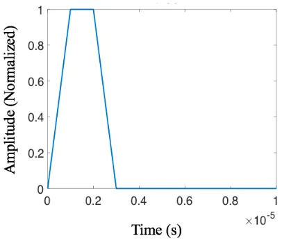
Figure 3.2 A rectangle pulse generated from MATLAB as the input signal at A. ... 63

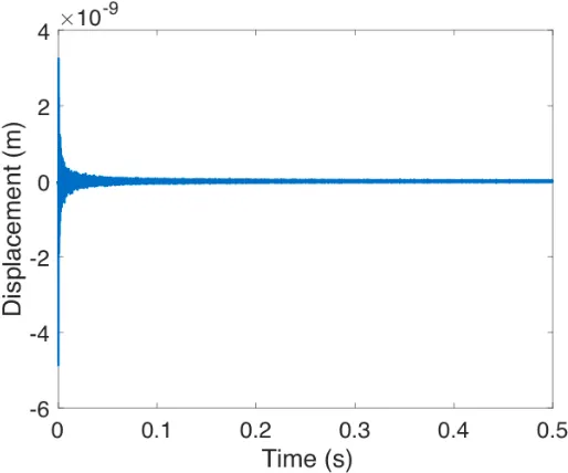
Figure 3.3 The received signal at Node 1 from the impulse source at A. ... 63

Figure 3.4 The 80 kHz - 120 kHz filtered signal at Node 1 from the impulse source at A. ... 64

Figure 3.5 Simulation layout for damage detection and localization using auto-correlation. ... ... 65

Figure 3.6 RGFs from (a) well-distributed sources, (b) sources in the left region, and (c) sources in the right region. ... 67

Figure 3.7 (a) Comparison between true Green’s function and reconstructed Green’s function from 300 partial reconstructed Green’s function. (b) Corresponding wave paths from point A to itself after Green’s function extraction. ... 68

Figure 3.8 The causal parts of the RGFs as a function of correlation time in the structure. Blue line for pristine case and red line for damaged case. ... 69

Figure 3.9 Damage localization using (a) AMV and (b) MSD methods in the simulation. ... 71

Figure 3.10 Uniform white noise programmed with Matlab as the excitation source. ... 71

ix Figure 3.12 Comparison between the true Green’s function and the reconstructed Green’s

function from position A to position B. Blue line indicating the true GF. Red line indicating the GF from the summation of the cross-correlation functions. ... 75 Figure 3.13 Diagram showing the number of arriving wave packets, corresponding to the

Figure 3.12. ... 75 Figure 3.14 Schematic diagram of a flat aluminum panel used in simulation. The red dot

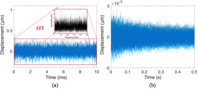
showing the location of the excitation source; the blue dot showing the location of signal retrieval. ... 77 Figure 3.15 (a) A uniform white noise signal input as the excitation source in the duration

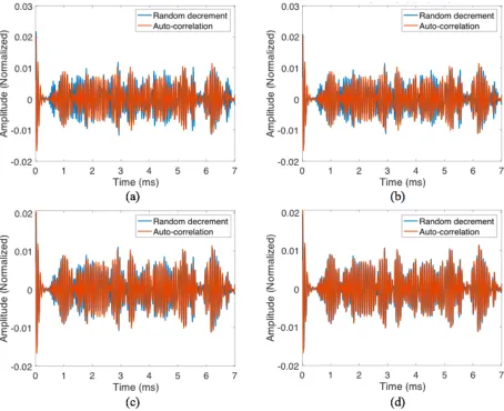
of 10 ms and its frequency spectrum shown in the upper right corner. (b) The extracted vertical displacement from the sensing location in Figure 3.14. ... 78 Figure 3.16 The comparison between the auto-correlation functions and the RD signatures.

The blue lines for RD signature and red lines for the auto-correlation function. (a) 1,000 (b) 2,500 (c) 5,000 (d) 10,000 averages for the RD signature... 80 Figure 4.1 Experiment setup using the air blow gun to excite the integral stiffened

aluminum panel and the laser Doppler vibrometer (LDV) to sense the response for long times. In actual experiments, the air blow gun was hand-held and the air pressure was randomly spread in all locations and angles. ... 87 Figure 4.2 Schematic diagram of an integral stiffened aluminum panel used in experiment.

x Figure 4.3 Comparisons of the causal parts of two RGFs as a function of correlation time

generated from auto-correlation of two separate measurements under different sensing time lengths at scanned position 8 in flat aluminum panel. (a) 0.01 (b) 0.2 (c) 4 (d) 8 seconds. The inserts showing zoom-in waveform from 0.5 to 4 ms correlation time. ... 89 Figure 4.4 Cross-correlation for RGFs of different sensing times with respect to RGF

from eight seconds sensing time. Cross-correlation result shown in blue dots and fitting curve in red line. The equation represents the mathematical fit with the curve. ... 90 Figure 4.5 Frequency response of air pressure blasting on the stiffened aluminum panel.

20.71 kHz and 45.74 kHz from harmonics of the LDV system. ... 90 Figure 4.6 The causal parts of the RGFs as a function of correlation time from different

locations in the flat aluminum panel. Blue line for pristine case and red line for damaged case. (a) Scanned point 7, and (b) Scanned point 22 to be shown in Figure 7. ... 93 Figure 4.7 Image intensity of a 90 mm × 90 mm region (represented by a 6 ´ 6 2-D array)

for the flat aluminum panel with simulated damage marked in white shaded area. Scanned points 7 and 22 corresponding to Fig. 6 (a) and (b) RGF positions. ... 94 Figure 4.8 The causal parts of the RGFs as a function of correlation time from different

xi Figure 4.9 Image intensity of a 90 mm ´ 90 mm area (represented by a 6 ´ 6 2-D array)

in the stiffened aluminum panel. The grey area indicating the geometry and location of the stiffener. The artificial damage location shown in white shaded rectangle region. Scanned point 11 and 20 corresponding to Fig. 6 (a) and (b) RGF positions. ... 96 Figure 4.10 Image intensity of a 90 mm ´ 90 mm area (represented by a 12 ´ 12 2-D array)

in the stiffened aluminum panel. The grey area indicating the geometry and the location of the stiffener. The artificial damage location shown in the white shaded rectangle. ... 96 Figure 5.1 Schematic diagram of a flat aluminum panel used in simulation. The red dot

showing the location of the excitation source; the blue dot showing the location of signal retrieval. ... 111 Figure 5.2 (a) A uniform white noise signal input as the excitation source in the duration

of 10 ms and its frequency spectrum shown in the upper right corner. (b) The extracted vertical displacement from the sensing location shown in Fig. 1. ... 111 Figure 5.3 The comparison between the auto-correlation functions and the RD signatures.

The blue lines for RD signature and red lines for the auto-correlation function. (a) 1,000 (b) 2,500 (c) 5,000 (d) 10,000 averages for the RD signature... 113 Figure 5.4 (a) Experiment setup with compressed air emitted from the 3-D printed nozzle

xii Figure 5.5 Frequency response of compressed air blasting on the stiffened aluminum

panel. 20.7 kHz and 45.7 kHz responses from harmonics of the LDV system... 116 Figure 5.6 Schematic diagram of an integral stiffened aluminum panel used in experiment.

(a) Isometric view of the panel, (b) the geometry and the dimensions of the panel, and (c) a 13 × 13 LDV scanned array in a 150 mm ´ 150 mm area which covers the simulated damage location marked by a shaded rectangle marked in yellow. ... 117 Figure 5.7 The GFs from the random decrement (RD) obtained at different locations in

the flat aluminum panel. The blue lines for pristine case and red lines for damaged case. (a) Scanning point #23. (b) Scanning point #32. (c) Scanning point #43 to be shown in Figure 8. ... 119 Figure 5.8 Image intensity of a 150 mm × 150 mm region (represented by a 13 ´ 13 2-D

array) for the flat aluminum panel with simulated damage marked in dark shaded area with black dashed line. Scanning points #23, #32, and #43 corresponding to Fig. 7 (a), (b) and (c) GF positions, respectively. ... 119 Figure 5.9 The GFs using RD from different locations in the stiffened aluminum panel.

The blue lines for the pristine case and red line for the damaged case. (a) Scanning point #1. (b) Scanning point #32. (c) Scanning point #55 to be shown in Fig. 10. ... 121 Figure 5.10 Image intensity of a 150 mm ´ 150 mm area (represented by a 13 ´ 13 2-D

xiii dark shaded rectangle region. Scanning points #1, #32 and #55 correspond to Fig. 9 (a), (b) and (c) GF positions, respectively... 122 Figure 5.11 Image intensity of a 150 mm ´ 150 mm area (represented by a 13 ´ 13 2-D

array) in the stiffened aluminum panel with a tilted damage shown in dark shaded rectangle. The shallow white area with black dashed line indicating the geometry and location of the stiffener. Whole image separated into three regions. ... 123 Figure 6.1 Passive sensing scheme via exploiting environmental loading from air flow

without much power consumption and recording structural responses using the embedded sensors to detect incipient abnormality. ... 131 Figure 6.2 (a) Experiment setup with 8 sensors and compressed air emitted from the

spraying nozzle to excite the integrally stiffened aluminum panel. (b) Detail dimension of the panel with the sensor number and wave paths of GFs used for damage localization. Yellow rectangle indicating the enlarged damage. ... 136 Figure 6.3 (a) The GFs of the sensor pair #1 and #3 from three measurements using 20

seconds recording signal. Waveform in negative time is the acausal part of the GF. (b) Comparison of GFs from the pristine and damaged stiffened panels. ... 138 Figure 6.4 (a) Damage image of a 150 mm × 150 mm region for the flat aluminum panel

xiv LIST OF TABLES

1 1. INTRODUCTION

1.1. Structural Health Monitoring

Traditionally, material testing methods such as tensile test, compression test, torsion test, impact test and bending test, etc. are all destructive in nature. These tests are all carried out on small number of samples (i.e. lot quality assurance sampling) to determine the material properties, e.g. Young’s modulus, yield and ultimate tensile strength, fatigue strength, fracture toughness and impact resistance, etc. To inspect the parts without compromising the structure serviceability, nondestructive testing (NDT) was introduced.

Nondestructive testing (NDT) have been used to inspect structures, including civil structures and aircraft structures, for their structural integrity. According to The American Society for Nondestructive Testing, nondestructive testing is defined as the process of “inspecting, testing, or evaluating materials, components or assemblies for discontinuities, or differences in characteristics without destroying the serviceability of the part or system.” In other words, the parts should remain the integrity when the nondestructive testing is completed.

Nondestructive testing (NDT) is often used interchangeably with nondestructive evaluation (NDE) or nondestructive inspection (NDI).

There are many types of NDT techniques and they are often referred to the type of equipment or of penetrating medium used in the test. These methods include, to name a few, visual inspection, acoustic emission testing, thermal-infrared testing, ultrasonic testing, vibration analysis, guided wave testing, electromagnetic testing, and radiographic testing, etc.

2 ground and drew into the hangar. It may require to disassemble or remove aircraft parts to conduct the NDT techniques. This significantly increase the airplane downtime, and thus reduce profit. Moreover, NDT is labor-intensive and thus increase the maintenance cost. Due to above reasons, NDT is often limited to the aircraft periodic maintenance checks or when defect or material degradation is suspected.

Structural health monitoring (SHM) offers the possibility to monitor the integrity of in-service aircraft in real-time. It often requires pre-installed on-board sensors to collect structural response from the environment (e.g. pressure change, turbulent flow), and operation loading (e.g. impact loading due to landing), or signals from the embedded actuators.

The advantages are multi-folds: 1) Increase the safety by detecting structure defects before a catastrophic failure happens. 2) It changes the scheduled and periodic maintenance to condition based maintenance, which reduces aircraft downtime and the maintenance cost, avoids dismantling the parts without defects, and involvement of human labor can be minimized. 3) optimize use of the aircraft structure1_.

3 Figure 1.1 Structural health monitoring system provides four levels of function accessing the

structural information.

A comprehensive structural health monitoring system consists of actuators, sensors, power supply and data processing center. Traditional wired sensors posts challenges on the application of SHM system, particularly for dense deployment of sensors on large-scale structures. High equipment costs, wiring and cabling and long installation time are main issues. Smart sensors have been proven to be able to solve these issues. Despite power consumption and reliability issues, smart sensors are defined with four advantages2_{: [1] on-board computing capability, [2] small size,} [3] wireless communication, [4] low cost. Researchers have proved that smart sensors could be potentially used for SHM with dense sensor array system3,4_.

4 SHM techniques can be applied to efficiently inspect the structure without costing too much energy, e.g., passive sensing techniques.

1.2. Passive Sensing

In the field of structural health monitoring (SHM), monitoring techniques can be broadly divided into two schemes: active and passive. Active scheme7,8 _{refers to the techniques involving}

using any form of actuators as sourcesand sensors to receive signal. The development of the active sensing technique for an autonomous structural health monitoring system usually requires a large amount of power consumption. While passive scheme is to use sensors only and without actuators, and it offers an opportunity to conduct real-time monitoring of the structure without the need of power-consuming system. More importantly, random and nonstationary environmental loading could be used to monitor the aircraft during the operation of the flight, minimizing the risks of the structural failure while maximizing the use of the machine.

Passive sensing have been researched to detect the impact locations or structural change 9-14_{. However, impact location algorithm, e.g., triangulation method, is not suitable for the damage} caused by fatigue or static loading, and studies in structural change identification is for global damage detection only. To compensate this drawback, imaging algorithms commonly used in active sensing15-17 _{can been incorporated to show possible damage locations.}

Reconstructed Green’s function (RGF) through correlation has been studied and shown great potential for helioseismology18,19_{, seismology}20-23 _{and ocean tomographic imaging}24-26_.

Duvall et al.14 _{first used cross-correlation to obtain direct and reflected acoustic waves between}

two points in helioseismology at 1993. They applied cross-correlation technique to observe the

acoustic wave propagation from the surface of the sun to the bottom of the cavity and back. They

5 annulus surrounding it. Up to three reflected waves were observed. The study also showed that

higher frequency (frequency range over 6.5 mHz) component of the acoustic wave contains little

information about reflected wave because the cutoff frequency of the acoustic wave for the

atmosphere is about 5.4 mHz. Besides cross-correlation, the study also applied auto-correlation in

wave traveling time/distance measurement. These concepts in fact are Green’s function

reconstruction techniques, in which auto-correlation and cross-correlation correspond to

self-Green’s function and self-Green’s function between two locations, respectively. In addition, Rickett and Claerbout19 _{compared the impulse response on the surface of the sun using cross-correlation} and Kolmogorov spectral factorization. The noise from the sun was recorded with Michelson Doppler Imager (MDI) and Acoustic wave propagation over 1.5 MHz frequency range was preserved. Although the focus is introducing spectral factorization in helioseismology, the study shows that by cross-correlating the noise traces recorded at two locations, impulse response between these two locations was constructed. Not only direct wave, but up to five multiple reflected waves were clearly visible.

7 to create a velocity map for the seismic tomography. Vertical component of surface response was

recording from a seismic array of 148 stations for 18 days. The arrays are distributed in Southern

California. The recorded signal was clipped to reduce the influence of large events. The frequency

range was chosen at 0.1 – 0.2 Hz. The results show that GFs from station pairs oriented

perpendicular to the coastline tend to be more stable than those from station pairs oriented parallel

to the coastline and have higher signal-to-noise ratio (SNR). The velocity map shows difference

of the arrival time at different regions, and the map correlates well with several geological features

in Southern California.

A study in Green’s function extraction for the civil structure was conducted by Snieder and

Safak23_{. Deconvolution was used to extract Green’s function from a library in California. The 43.9}

m tall building with additional 4.3m deep basement was subjected to an seismic event and 10 floors

of the structural response were recorded. Fundamental theory was established for the building’s

basic response (Green’s function) extraction avoiding the ground coupling. Derivation of the

normal modes of the building was also obtained for the intrinsic attenuation and the shear wave

velocity estimation. It shows that deconvolution with the top floor rendered upgoing and

downgoing waves, while deconvolution with the basement gave upgoing wave only and the

fundamental mode of the building. The results showed that the Green’s function extracted was

independent with the excitation source. Wave arrival times of the Green’s functions from different

floors gave a fairly good estimation of shear wave velocity comparing to the theory. Whereas the

ratio of the amplitude of the Green’s functions for floor 1-3 was used to estimate the attenuation

of the structure, and is in good agreement with the theoretical value.

8 using vertical hydrophones in the ocean were conducted. The 20 mins of data from hydrophone arrays was recorded and further filtered between 70 and 130 Hz. The result shows that the deterministic wave fronts can be recovered through the cross-correlation of the signal under environmental acoustic noise (e.g. a collapsing of bubble), provided long-time correlation. The study suggests that the signal-to-noise ratio (SNR) of the Green’s function is related to the noise sources position, in which attenuation of the wave propagation in the medium and the transmission angle between noise and two receivers are important. Correlation time and frequency bandwidth were also shown to affect the SNR. In another study, Siderius et al.25 _{utilized passive imaging via} cross-correlation to determine water depth and seabed sub-bottom layering. In the first experiment,

a fixed array of 33 hydrophones with 0.5 m spacing in 200 – 1500 Hz frequency range was used

to measure the distance between the hydrophone and the water depth. The estimation from the

ambient noise cross-correlation matches well with the one from the geo-acoustic inversion

experiment. In the second experiment, 32 hydrophones spaced 0.18 m drifting freely in the ocean,

and 70 seconds data in 50 – 4000 Hz range was used for a single fathometer time trace. A seismic

boomer (sonar) was used to profile the seabed sub-bottom and the strongest relfectors from the

seabed. The fathometer processing through cross-correlation from ambient ocean noise produced

a bathymetry very closed to the one created by the sonar.

For the smaller scale of the experiment, the same phenomenon was also observed. Lobkis and Weaver27 _{derived normal modes based theory for cross-correlation of the signals from the}

9 function from a single mode. Deconvolution was used to decouple the source function. In the experiment, ultrasonic acoustic signal was generated in an irregular aluminum alloy block and it was proved that waveform from averaging cross-correlation could be similar to that from direct pitch-catch result. The link between the study and the work by Roux et al.24 _{is volume distributed} sources were used by Weaver and Lobkis for experiments on metal block, while the application in Roux et al.’s study was for naval passive tomographic imaging.

Snieder28 _{derived detailed theory for cross-correlation passive sensing based on wave}

constructive interference from the defects. Cross-correlation of the scattered waves radiated from the defects sensed at two receiver locations results in a waveform including the ballistic wave (the first arrival wave) between two receivers. In this study, theory was extended from ballistic wave to surface wave, and relaxed the condition from closed medium to open medium. Stationary phase approximation was incorporated in the theory to cancel the oscillatory term, which is contributed due to the scatterer (wave source) present far away from the straight line between two receivers. This proves that the constructive part of the cross-correlation eventually forms the ballistic part in Green’s function. The similar concept was also appeared in other studies25,26_{, which states that the}

source firing direction has to overlap with the direction between two receivers to extract the Green’s function. The artifacts (spurious arrival of wave) may appear if the source firing direction is not overlap with any of the wave propagation path between the receivers29,30_.

Wapenaar31 _{showed that elastodynamic Green’s function between two locations can be}

10 positions are all the same, which leads to that no separate measurements are needed to correlate the response from all the sources to obtain the Green’s function, relaxing the condition indicated in the study by Van Wijk29_{. The band-limited source leads to the band-limited Green’s function} was also implicitly derived. It was shown that diffusive wavefield is not a requirement for reconstructing a perfect Green’s function, especially for the ballistic wave (the first arrival).

The maturity of the theory of Green’s function extraction via cross-correlation28,31,32 _and its deployment in multiple research fields leaded it to the initial exploring of passive sensing in structural health monitoring33-37_{. Sabra et al.}33 _{reconstructed Green’s function from a pair of} accelerometers mounted in a flat plate (12.9 m ´ 3.05 m ´ 18.4 cm) with stainless steel skins and a bronze hydrofoil (2.134 m ´ 3.05 m ´ 17.1 cm) subjected to vibration noise caused by turbulent flow (flow speed 20 m/s). Impulse response from the active sensing was compared with that from the cross-correlation on the first plate. Signal whitening for estimated GF on 900 – 1200 Hz frequency band component was compared and the match between two GFs was good. For the hydrofoil, GFs in low frequency 100 - 250 Hz showed identical trend, however, GFs in 800 – 1500 Hz frequency range were different in character and magnitude due to changes in mounting conditions. In another study, Moulin et al.36 _{used localized (fixed) acoustic sources from a} loudspeaker rather than distributed sources for Green’s function extraction, which could be possibly used in the case where operational loading is caused by the engine. The wave path was then not covering the whole structure, causing some “partially” reconstructed Green’s function. The experimental results from a 200 mm ´ 100 mm ´ 6 mm aluminum panel with a simulated defect shows that partially reconstructed Green’s function is still able to be used in damage

11 source distribution types to the SNR ratio of the extracted Green’s function. The panel was cut intentionally into an irregular shape to expedite the formation of diffusive wavefield. A laser Doppler vibrometer (LDV) was used to extract out-of-plane velocity of the panel at 610 sensing points, and two PZT actuators were used to excite a short sinusoidal pulse, respectively. The results shows that the level of signal clipping around 15 times of the noise level gave the best of SNR ratio for the Green’s function. The number of the excitation sources and duration of the signal time for cross-correlation positively correlated with the SNR of the Green’s function. The source distribution types affected little to the Green’s function as fully diffusive wavefield was achieved. Phase and group velocity from the reconstructed Green’s function (RGF) matched the predicted value given sufficient amount of sources. The RGF through cross-correlation was shown providing a new way for remotely and passively monitoring a local area in complex structures.

Cross-correlation for Green’s function extraction only provides an alternative to reconstruct wave signal between two points. For damage detection purpose in structural health monitoring, Green’s function comparison between the pristine and damaged structures is needed, and often statistical tool for quantitively assessment is necessary38_{. On the other hand, for damage} localization purpose, imaging algorithm or strategy is required on top of the tools required for damage detection39-44_{. In the studies by Chehami et al.}39,40_{, flexural wave based theory for RGF} was derived, which consider out-of-plane displacement based on Kirchhoff-Love equation and a limited number of sources. In numerical experiment, identical short pulses of noise were generated in an aluminum panel and the cross-correlation technique was applied. The RGF from pristine structure was subtracted by that from damaged structures to produce scattered wave signal only, which represents the wave from the damage only. Time-reversal imaging41 _{was used to map the}

12

´ 500 mm ´ 3 mm aluminum plate was conducted for damage localization with 8 piezoelectric

transducers as sensors covering a circular area (300 mm in diameter). Sinusoidal 20 kHz pulse from 20 piezoelectric transducers, friction noise from the scrubbing pad and acoustic noise from the loudspeaker were the sources. Signal-processing tool included pulse-compression, normalization prior to cross-correlation, and signal whitening for signal duration from 40 ms to 60 seconds. Four types of simulated damage were tested: hole, neodymium cylinder inclusion, surface crack and through-crack. Same imaging condition (Time-reversal) was applied to accurately map the damage location. To apply passive sensing through cross-correlation in aircraft structure, the dynamic nature of the excitation source must be taken into account. Hence, stably GFs in different measurements with random source are necessary for such technique. Scalea et al.43 _{inspected a}

railroad track with fully non-contact, passive-only system mounted on a running train which continuously generates random and non-stationary signal. Two air-coupled receivers separated by about 45 cm were used to capture the noise centered at 120 kHz for inspection purpose. The system Deconvolution operator added in cross-correlation was proposed to extract Green’s function from dynamic excitation to the rail to remove the coupling (or transfer function) of receivers and the section between the noise source and the receiver. A damage index provided a quantitative way to show the discontinuity in the rail, including welds, joints and defects. Since the rail can be considered as a 1-D problem, defect locations were shown once the damage indices were created.

13 been used in a few studies44-47_{. To distinguish, Green’s function from cross-correlation will be} mentioned as Green’s function, and Green’s function from auto-correlation will be mentioned as self-Green’s function hereafter. Hadziioannous et al.46 _{compared the self-Green’s function} extracted from auto-correlation (passive sensing) with the signal from the pulse-echo method

(active sensing). A 64 mm ´ 80 mm bulk gel with large amount of air bubbles was used to mimic

the seismology study and ultrasonic pulse (2.5 MHz) was emitted through transducers. Velocity

variation in the late stage of wave propagation (coda wave) due to temperature change was

obtained using signal stretching and doublet techniques. It was found that the velocity variation

was the same for both active and passive sensing, although extracted self-GF was not converged

to the true self-GF from the pulse-echo measurement. This study aimed to provide more insight

for seismology through small-scale, controllable experiment. The auto-correlation sensitivity for

the change of the medium state does show potential of such technique in structural health

monitoring.

14 Vandiver et al.49 _{derived a rigorous mathematical proof for the random decrement} technique. The author showed that for a Gaussian random excitation source, a random decrement signature of a measured long time signal is proportional to the auto-correlation function of that recorded signal. The triggering level and magnitude of the auto-correlation function at zero lag were found to be related to the proportion between the auto-correlation function and RD signal. Random decrement technique was tested on an offshore structure where acceleration response was measured. After averaging over 80 times of RD signatures, it was found the waveform of the random decrement signal approaches to the causal part of the correlation function (i.e. auto-correlation function in the positive time scale).

Curadelli et al.51 _{used the random decrement to obtain free vibrational decay below 10 Hz} for damping evaluation. Horizontal acceleration from the top floor of a one bay, six-storey aluminum 3-D frame model (0.5 m tall and 0.1 m wide) was processed with random decrement, and wavelet transform was used to acquire instantaneous damping coefficient for damage detection. The structure was subjected to Gaussian white noise using a shaking table to create unidirectional base motion. The study showed that parameters characterizing damping properties could be used as damage-sensitive features, and RD based structural response retrieval could assist damage detection process.

15 excitation. The RD was shown to consistently reconstruct the structural response and thus improves the outlier detection process. The author noted that the methodology is capable of detection changes in the structures for most of the cases.

Sim et al.53 _{implemented random decrement in wireless sensor network for structural} feature extraction. It was demonstrated that the RD technique with decentralized data aggregation reduces computational effort significantly comparing to Natural Excitation Technique (NExT). A simply supported truss model was simulated with 0-150 Hz band-limited white noise excitation. For experimental verification, a truss structure consisting of steel hollow circular tubes was tested with 0-100 Hz white noise. Mode shapes and natural frequency were reconstructed and calculated for both cases. It was found that the RD saves about 22% and 28% amount of data transferred which is required for structural properties calculation in simulation and experiment, respectively. This is because the RD only needs trigger information instead of the entire signal.

1.3. Objective and Scope

It is cleared from the literature review that correlation-based Green’s function extraction technique has been widely used in helioseismology, seismology and ocean tomographic imaging. However, the studies in the aircraft structures are still limited. Although the theoretical and some simulation works have been published, there are still gaps needed to be bridged for the aircraft structures. As for the Random decrement, the application of the RD in aircraft structure is rare, and the focus has been on vibration features at low frequencies.

16 structures subjected to the turbulent flow (including aluminum and composite structures) will also be shown.

17 1.4. References

[1] D. Balageas, “Introduction to Structural Health Monitoring,” Structural Health Monitoring,

pp.13-43, 2006.

[2] B.F. Spencer Jr, M.E. Ruiz-Sandoval, and N. Kurata, “Smart Sensing Technology:

Opportunities and Challenges,” Structural Control and Health Monitoring, vol. 11, no. 4, pp.

349-368, 2004.

[3] S. Jang, H. Jo, S. Cho, K. Mechitov, J. A. Rice, S. H. Sim, H. J. Jung, C. B. Yun, B. F.

Spencer Jr, and G. Agha, “Structural Health Monitoring of A Cable-Stayed Bridge using

Smart Sensor Technology: Deployment and Evaluation,” Smart Structures and Systems, vol.

6, no. 5-6 , pp. 439-459, 2010.

[4] S. Cho, H. Jo, S. Jang, J. Park, H. J. Jung, C. B. Yun, B. F. Spencer Jr, and J. W. Seo,

“Structural Health Monitoring of A Cable-Stayed Bridge using Wireless Smart Sensor

Technology: Data Analyses. Smart Structures and Systems, vol. 6, no. 5-6, pp. 461-480,

2010.

[5] L. Wang and F. G. Yuan, “Vibration Energy Harvesting by Magnetostrictive Material. Smart

Materials and Structures, vol. 17, no. 4, p.045009, 2008.

[6] S. Palagummi and F. G. Yuan, “An Efficient Low Frequency Horizontal Diamagnetic

Levitation Mechanism based Vibration Energy Harvester,” International Society for Optics

and Photonics, vol. 9799, p. 97991O. 2016.

[7] H. Y. Chang and F. G. Yuan, “Damage Imaging in A Stiffened Curved Composite Sandwich

18 [8] H. Y. Chang and F. G. Yuan, "Damage Visualization of Scattered Ultrasonic Wavefield via Integrated High-speed Camera System," International Workshop on Structural Health Monitoring, 2019. Submitted.

[9] H A. Cole, “On Line Failure Detection and Damping Measurement of Aerospace Structures

by RD signatures,” NASA, 1973.

[10] M. Gul and F. N. Catbas, “Statistical Pattern Recognition for Structural Health Monitoring

using Time Series Modeling: Theory and Experimental Verifications,” Mechanical Systems

and Signal Processing, vol. 23, no. 7, pp. 2192-2204, 2009.

[11] W. J. Staszewski, S. Mahzan, and R. Traynor, “Health Monitoring of Aerospace Composite

Structures–Active and Passive Approach,” Composites Science and Technology, vol. 69, no.

11-12, pp. 1678-1685, 2009.

[12] K. Choi and F. K. Chang, “Identification of Impact Force and Location using Distributed Sensors,” AIAA journal, vol. 34, no. 1, pp. 136-142, 1996.

[13] S. Mahzan, W. J. Staszewski, and K. Worden, “Experimental Studies on Impact Damage Location in Composite Aerospace Structures using Genetic Algorithms and Neural

Networks,” Smart Structures and Systems, vol. 6, no. 2, pp. 147-165, 2010.

[14] M. Faisal Haider, A. Migot, M. Bhuiyan, and V. Giurgiutiu, “Experimental Investigation of

Impact Localization in Composite Plate Using Newly Developed Imaging

Method,” Inventions, vol. 3, no. 3, p. 59, 2018.

[15] C. Wang, J. Rose, F. Chang, “A Synthetic Time-Reversal Imaging Method for Structural

Health Monitoring,” Smart Materials and Structures, vol. 13, no. 2, pp.415, 2004.

19 [17] X. Zhao, H. Gao, G. Zhang, B. Ayhan, F. Yan, C. Kwan, and J. Rose, “Active Health Monitoring of An Aircraft Wing with Embedded Piezoelectric Sensor/Actuator Network: I.

Defect Detection, Localization and Growth Monitoring,” Smart Materials and

Structures, vol. 16, pp. 1208, 2007.

[18] T. Duvall Jr, S. Jeffferies, J. Harvey, and M. Pomerantz, “Time–Distance

Helioseismology,” Nature, vol. 362, no. 6419, p.430, 1993.

[19] J. Rickett and J. Claerbout, “Acoustic Daylight Imaging via Spectral Factorization:

Helioseismology and Reservoir Monitoring,” The Leading Edge, vol. 18, no. 8, pp. 957,

1999.

[20] M. Campillo and A. Paul, “Long-Range Correlations in the Diffuse Seismic

Coda,” Science, vol. 299, no. 5606, pp. 547-549, 2003.

[21] N. M. Shapiro, M. Campillo, L. Stehly and M.H. Ritzwoller, “High-Resolution

Surface-Wave Tomography from Ambient Seismic Noise.” Science, vol. 307, no. 5715, pp.1615 -

1618, 2005.

[22] K. G. Sabra, P. Gerstoft, P. Roux, W. A. Kuperman, and M.C. Fehler, “Surface Wave

Tomography from Microseisms in Southern California,” Geophysical Research Letters, vol.

32, no. 14, 2005.

[23] R. Snieder and E. Safak, “Extracting the Building Response using Seismic Interferometry:

Theory and Application to The Millikan Library in Pasadena,” California. Bulletin of the

Seismological Society of America, vol. 96, no. 2, pp. 586-598, 2006.

[24] P. Roux, W. Kuperman, and NPAL Group, “Extracting Coherent Wave Fronts from Acoustic

Ambient Noise in the Ocean,” The Journal of the Acoustical Society of America, vol. 116,

20 [25] M. Siderius, C. H. Harrison, and M. B. Porter, “A Passive Fathometer Technique for Imaging

Seabed Layering using Ambient Noise,” The Journal of the Acoustical Society of

America, vol. 120, no. 3, pp. 1315-1323, 2006.

[26] K. G. Sabra, P. Roux, and W. A. Kuperman, “Arrival-Time Structure of The Time-Averaged

Ambient Noise Cross-Correlation Function in An Oceanic Waveguide,” The Journal of the

Acoustical Society of America, vol. 117, no. 1, pp. 164-174, 2005.

[27] O. I. Lobkis and R. L. Weaver, “On the Emergence of the Green’s Function in the Correlations of a Diffuse Field,” The Journal of the Acoustical Society of America, vol. 110, no. 6, pp. 3011-3017, 2001.

[28] R. Snieder, “Extracting the Green’s Function from the Correlation of Coda Waves: A Derivation Based on Stationary Phase,” Physical Review E, vol. 69, no. 4, p. 046610, 2004. [29] K. Van Wijk, “On Estimating The Impulse Response between Receivers in A Controlled

Ultrasonic Experiment,” Geophysics, vol. 71, no. 4, pp. SI79-SI84, 2006.

[30] R. Snieder, K. Van Wijk, M. Haney, and R. Calvert, “ Cancellation of Spurious Arrivals in Green’s Function Extraction and the Generalized Optical Theorem,” Physical Review E, vol. 78, no. 3, p.036606, 2008.

[31] K. Wapenaar, “Retrieving the Elastodynamic Green's Function of an Arbitrary Inhomogeneous Medium by Cross Correlation,” Physical Review Letters, vol. 93, no. 25, p. 254301, 2004.

[32] K. Wapenaar and J. Fokkema, “Green’s Function Representations for Seismic

Interferometry,” Geophysics, vol. 71, no. 4, pp. SI33-SI46, 2006.

[33] K. G. Sabra, E. S. Winkel, D. A. Bourgoyne, B. R. Elbing, S. L. Ceccio, M. Perlin, and D.

21 Estimate the Structural Impulse Response. Application to Structural Health Monitoring,” The Journal of the Acoustical Society of America, vol. 121, no. 4, pp. 1987-1995, 2007.

[34] K. G. Sabra, A. Srivastava, F. Lanza di Scalea, I. Bartoli, P. Rizzo, and S. Conti, “Structural

Health Monitoring by Extraction of Coherent Guided Waves from Diffuse Fields,” The

Journal of the Acoustical Society of America, vol. 123, no. 1, pp. EL8-EL13, 2008.

[35] E. Larose, P. Roux, and M. Campillo, “Reconstruction of Rayleigh–Lamb Dispersion

Spectrum based on Noise Obtained from an Air-Jet Forcing,” The Journal of the Acoustical

Society of America, vol. 122, no. 6, pp. 3437-3444, 2007.

[36] E. Moulin, N. Abou Leyla, J. Assaad, and S. Grondel, “Applicability of Acoustic Noise

Correlation for Structural Health Monitoring in Nondiffuse Field Conditions.” Applied

Physics Letters, vol. 95, no. 9, p.094104, 2009.

[37] A. Duroux, K. G. Sabra, J. Ayers, J. and M. Ruzzene, “Extracting Guided Waves from

Cross-Correlations of Elastic Diffuse Fields: Applications to Remote Structural Health

Monitoring. The Journal of the Acoustical Society of America, vol. 127, no. 1, pp. 204-215,

2010.

[38] J. D. Tippmann and F. Lanza di Scalea, “Passive-Only Damage Detection by Reciprocity of

Green’s Functions Reconstructed from Diffuse Acoustic Fields with Application to Wind

Turbine Blades,” Journal of Intelligent Material Systems and Structures, vol. 26, no. 10, pp.

1251-1258, 2015.

[39] L. Chehami, E. Moulin, J. de Rosny, C. Prada, O. B. Matar, F. Benmeddour and J. Assaad,

“Detection and Localization of a Defect in a Reverberant Panel using Acoustic Field

22 [40] L. Chehami, J. De Rosny, C. Prada, E. Moulin, and J. Assaad, “Experimental Study of

Passive Defect Localization in Plates using Ambient Noise,” IEEE transactions on

Ultrasonics, Ferroelectrics, and Frequency Control, vol. 62, no. 8, pp. 1544-1553, 2015. [41] J. E. Michaels and T. E. Michaels, “Guided Wave Signal Processing and Image Fusion for

in situ Damage Localization in Panels,” Wave Motion, vol. 44, no. 6, pp. 482-492, 2007.

[42] Y. Yang, L. Xiao, W. Qu, and Y. Lu, “Passive Detection and Localization of Fatigue

Cracking in Aluminum Plates using Green’s Function Reconstruction from Ambient

Noise,” Ultrasonics, vol. 81, pp. 187-195, 2017.

[43] F. di Scalea, X. Zhu, M. Capriotti, A. Liang, S. Mariani and S. Sternini, “Passive Extraction of Dynamic Transfer Function from Arbitrary Ambient Excitations: Application to High-Speed Rail Inspection from Wheel-Generated Waves,” Journal of Nondestructive Evaluation,

Diagnostics and Prognostics of Engineering Systems, vol. 1, no. 1, p. 011005, 2018.

[44] S. Ohmi, K. Hirahara, H. Wada, and K. Ito, “Temporal Variations of Crustal Structure in the

Source Region of the 2007 Noto Hanto Earthquake, Central Japan, with Passive Image Interferometry,” Earth, planets and space, vol. 60, no. 10, pp. 1069-1074, 2008.

[45] S. Minato, T. Tsuji, S. Ohmi, and T. Matsuoka, “Monitoring Seismic Velocity Change Caused by the 2011 Tohoku Oki Earthquake using Ambient Noise Records,” Geophysical

Research Letters, vol. 39, no. 9, 2012.

23 [47] X. Li, J. Chi, D. Gao, J. Li, and N. Wang, “Extraction of Scattering Echo Time by Surf Noise Background Subtracted Autocorrelation. The Journal of the Acoustical Society of

America, vol. 142, no. 1, pp. EL1-EL6, 2017.

[48] H A. Cole, “On Line Failure Detection and Damping Measurement of Aerospace Structures by RD signatures,” NASA, 1973.

[49] J.K. Vandiver, A.B. Dunwoody, R.B. Campbell and M.F. Cook, “A Mathematical Basis for the Random Decrement Vibration Signature Analysis Technique,” Journal of Mechanical

Design, vol. 104, pp. 307, 1982.

[50] R. Brincker, S. Krenk, P.H. Kirkegaard and A. Rytter, “Identification of Dynamical Properties from Correlation Function Estimates,” Bygningsstatiske Meddelelser, vol. 63, no. 1, pp. 1-38, 1992.

[51] R.O. Curadelli, J.D. Riera, D. Ambrosini and M.G. Amani, “Damage Detection by Means of Structural Damping Identification,” Engineering Structures, vol. 30, no. 12, pp. 3497-3504, 2008.

[52] M. Gul and F.N. Catbas, 2009. “Statistical Pattern Recognition for Structural Health Monitoring using Time Series Modeling: Theory and Experimental

Verifications,” Mechanical Systems and Signal Processing, vol. 23, no. 7, pp. 2192-2204, 2009.

[53] S.H. Sim, J. F. Carbonell-Márquez, B.F. Spencer Jr and H. Jo, “Decentralized Random Decrement Technique for Efficient Data Aggregation and System Identification in Wireless Smart Sensor Networks,” Probabilistic Engineering Mechanics, vol. 26, no. 1, pp. 81-91, 2011.

24 2. FORMULATIONS OF GREEN’S FUNCTION RECONSTRUCTION METHODS AND

IMAGING CONDITION

This chapter document the formulations of the Green’s function extraction techniques, including auto-correlation, cross-correlation, and random decrement, for the passive sensing application. The second part of this chapter will present the imaging conditions that was created from the other studies, or specifically developed for this research.

2.1. Formulations of Green’s Function Reconstruction Methods

The Green’s function extraction techniques was formulated based on the equation of motion, reciprocity theorem, and the representation theorem. This section will detail the derivations of each theory and concept.

2.1.1. Equation of motion

In this chapter, some fundamental results for time-reversal method used in impact identification and damage detection are derived. They are based on the integral representation of the solution of the elastic wave equation. The following section underlying the physics of the representation theorem in terms of Green’s functions based on linear elastodynamics is formulated. The time-reversal method is one of the most popular methods for optimally focusing the damage(s) from sensor data. The detailed proof can be seen from Aki and Richards1_.

Consider an initial-boundary value problem of generation of wave in an elastic material. The elastic property can be described by the elastic tensor (or material stiffness matrix)

and density . The material properties (i.e. elastic tensor and density) considered here are only the functions of the position, instead of the time. The region of interest is in the domain D, enclosed by a surface S. The equation of motion in time domain is given below:

, , (2.1)

C_ijkl(x)

ρ(x)

25 where , , and are stress tensor, displacement and body force, respectively. The notation

is used to express spatial derivative , in the direction,. Double dots over a variable

indicate a second-order time derivative. In addition, stress tensor can be written as ,

where is the strain tensor. Note that in the time domain, is a function of the

time and the position , i.e., .

An important property of the elastic tensor is that the elastic tensor is symmetric:

(2.2) The stress tensor can be expressed as

(2.3)

Using , Equation (2.3) becomes

Exchange the notation l and k for the second term on the right-hand side,

Finally, the stress tensor can be written as

From above results, rewrite Equation (2.1) as

(2.4)

σ_ij u_i f_i

()_,i ∂

∂x_i i

σ_ij=C_ijklε_kl

ε_kl =1

2(uk,l+ul,k) u

t x u(x,t)

C_ijkl =C_klij=C_ijlk =C_jikl.

σ_ij=C_ijklε_kl

C_ijklεkl = 1

2Cijkluk,l+ 1

2Cijklul,k.

C_ijkl =C_ijlk

1

2Cijkluk,l+

1

2Cijklul,k =

1

2Cijkluk,l+

1

2Cijlkul,k.

1

2Cijkluk,l+ 1

2Cijkluk,l =Cijkluk,l.

σ_ij=C_ijklu_k,l.

26 The equation shows that the particle movement (acceleration in this case) is caused by the disturbance in or outside of the medium. The medium can be excited from any one of the three sources of disturbance: body force, initial condition, and boundary condition. The elastic waves with wave front travel through the medium from the source of disturbance. The particle movement can be expressed by mathematical form of particle displacement in the equation of motion, i.e. Equation (2.4).

The body force term can be expressed simply by the notation , in which i is the direction of the force applied. The boundary condition can be divided into two groups, i.e., the displacement and the traction boundary conditions that are given at each point of the surfaces S,

. For the displacement boundary condition, for , where is the prescribed displacement. For the traction boundary condition, for . The boundary condition can also be a combination of the two at part of the boundary.

Initial condition needs to be considered. The particle displacement and its derivative with respect to time are given at some starting value, . It gives that , and

, for .

One way to solve the wave problems is using partial differential equations. Another way to see the problem is through equivalent integral equation, representing the displacement response from the initial and boundary conditions and the body force.

2.1.2. Reciprocity theorem

The waveform excited at position B by an actuator received at position A by a sensor, is equal to the waveform excited at position A by an actuator received at position B by a sensor. This is called the principle of reciprocity. From the point of view of physics, it means that the energy

u(x,t)

f_i(A)_(x,t)

S=S_u∪S_σ u_i(x,t)=u_i(x,t) x∈S_u u_i(x,t)

t_i =C_ijklu_k,ln_j x∈S_σ

u(x,t)

t=t₀ u(x,t₀)=u₀(x)

!

27 absorption and particle interaction along the wave propagation path from A to B is the same as those from B to A.

The principle of reciprocity is a powerful tool. It simplifies many of the mathematical derivations, and reduces significant amount of resources and time for some of time-consuming simulations and experiments. For example, it is common to use the combination of laser Doppler vibrometer (LDV) and Nd:YAG pulse laser to inspect the structural integrity. Laser Doppler vibrometer detects the out-of-plane velocity and is used to scanned the surface of the structure. Nd:YAG pulse laser system can focus a laser beam on the surface and heat up the surface in a short time, creating a thermal expansion in the local area and generating elastic wave in the structure. However, it is time-consuming to use LDV to scan the surface as sensor system while pulse laser acts as an actuator, which mimics a sensor array collecting signal excited from an single sensor, due to the fact that LDV system need to refocus every time it moves to a new position. The alternative way is to utilize reciprocity theorem, where pulse laser is used to excite at an array of points on the surface of the structure and LDV measures the same point continuously. Since pulse laser system does not require refocus, it reduces the experiment time significantly.

This section deals with the derivation of the reciprocity theorem.

Let two permissible states A and B occur in the same medium. Same as the previous assumption, here assume is the particle displacement due to the body force , boundary conditions on the surface S and initial condition at . Assume another particle movement caused by a different body force , boundary conditions on the surface S

and initial conditions at . The equation of motion for two states, using Equation (2.4), are given by:

(2.5)

u(A)_{(x,t) f}(A)

t=0

u(B)_{(x,t) f}(B)

t=0

(C_ijklu_k,l(A)₎ ,j+ fi

28 (2.6)

Multiplying Equation (2.5) by and Equation (2.6) by , subtracting two equations, rearranging and adding integral over volume V on two equations gives

. (2.7)

Using integral by parts, the first term of Equation (2.7) can be given by

, (2.8)

and the second term can be expressed using the same method,

. (2.9)

Note that due to symmetric property of elastic tensor, , the second term on the right-hand side of Equation (2.8) can be rewritten as

. It gives,

,

which is exactly the second term on the right-hand side of Equation (2.9).

By inserting Equation (2.8) and Equation (2.9) back into Equation (2.7), and using Gauss’s theorem to convert volume integral into surface integral, and considering the symmetry of elastic tensor, Equation (2.7) leads to

.(2.10)

Equation (2.10) can be expressed in the vector form, (C_ijklu_k(_,B_l)₎

,j+ fi

(B) _=ρu!! i (B)

u_i(B) _u

i (A)

u_i(B)_(C

ijkluk,l

(A)₎ ,j−ui

(A)_(C

ijkluk,l

(B)₎ ,j

⎡⎣ ⎤⎦dV =− u_i(B)_(f

i

(A)_−ρu!!

i

(A)_)−u

i

(A)_(f

i

(B)_−ρ!!u

i

(B)_)dV

V

∫

∫

u_i(B)_(C ijkluk,l

(A)₎

,jdV

V

∫

= (u_i(B)_C ijkluk,l

(A)₎

,jdV

V

∫

− u_i,j(B)_C ijkluk,l

(A)_dV

V

∫

u_i(A)_(C

ijkluk,l

(B)₎ ,jdV V

∫

= (u_i(A)_C

ijkluk,l

(B)₎ ,jdV V

∫

− u_i(_,A_j)_C

ijkluk,l

(B)_dV

V

∫

C_ijkl =C_klij

u_i(_,B_j)_C

ijkluk,l

(A)_=u

i,j

(B)_C

klijuk,l

(A)

u_i(_,B_j)_C

klijuk,l

(A)_=u

k,l

(A)_C

klijui,j

(B)

(u_i(B)_C ijkluk,l

(A)_)−(u i (A)_C

ijkluk,l (B)₎

⎡⎣ ⎤⎦n_jdS

S

!

∫

i

(A)_−ρu!! i (A)_)−u

i (A)_(f

i

(B)_−ρu!! i (B)_)dV

V

29

, (2.11)

where the ith _{component of the traction vector t is . This is so called the Betti’s} reciprocity theorem.

The above equations do not yet utilize the initial conditions. Further, Equation (2.11) holds when the states (A) and (B) are evaluated at different times. Set time in state (A) at and time in state (B) at , and integrate Equation (2.11) over the time from 0 to , Equation (2.11) becomes

(2.12)

Take the time integration first, then the acceleration term can be linked with the initial and final times,

(2.13)

The integral cancel out with the derivative, and Equation (2.13) becomes

(2.14)

Rearrange the equation and it gives

(2.15)

(u(B)_t(A)_)−(u(A)_t(B)_)dS

S

!

∫

V

∫

t_i =C_ijklu_k,ln_j

t(A)_=t

t(B)_{=τ−t τ}

u(B)_{(τ −t)t}(A)_(t)

⎡⎣ ⎤⎦− u(A)_(t)t(B)_(τ−t)

⎡⎣ ⎤⎦dS

S

!

∫

0 τ

∫

= − u(B)_{(τ −t) f}(A)_(t)−ρu!!(A)_(t)

⎡⎣ ⎤⎦−u(A)_{(t) f}(B)_{(τ−t)−ρu!!}(B)_(τ−t)

⎡⎣ ⎤⎦dV

V

∫

0 τ

∫

−u(B)_{(τ−t)ρ!!u}(A)_(t)+u(A)_(t)ρu!!(B)_(τ−t)dt 0

τ

∫

∂t −u

(B)_{(τ −t)u!}(A)_(t)+u(A)_(t)u!(B)_{(τ −t)}

⎡⎣ ⎤⎦dt

0 τ

∫

ρ ∂

∂t −u

(B)_(τ−t)u!(A)_(t)+u(A)_(t)u!(B)_(τ−t)

⎡⎣ ⎤⎦dt

0

τ

∫

=ρ −u(B)

(0)u!(A)

(τ)+u(A)

(τ)u!(B)

(0)+u(B)

(τ)u!(A)

(0)−u(A)

(0)u!(B)

(τ)

⎡⎣ ⎤⎦.

ρ −u(B)_(0)u!(A)_(τ)+u(A)_(τ)u!(B)_(0)+u(B)_(τ)u!(A)_(0)−u(A)_(0)u!(B)_(τ)

⎡⎣ ⎤⎦

=ρ −u!(A)_(τ)u(B)_(0)+u(A)_(τ)u!(B)_(0)+u!(A)_(0)u(B)_(τ)−u(A)_(0)u!(B)_(τ)