Computational Study of Grain Boundaries and Nano-Reactive Materials

ABSTRACT

LU, SHIJING. Computational Study of Grain Boundaries and Nano-Reactive Materials. (Under the direction of Professor Donald Brenner.)

The thesis summarized my research efforts in two areas:

Chapters 1 to 4 devote to the computational study of grain boundary (GB) structure, energy and mobilities. Despite of the considerable effort that has been placed on those topics, computational study of GB is still a daunting task. Chapter 1 gives a small glimpse into the rich world of GB studies in the past and the difficulties they met. In chapter 2, we propose a new approach to predicting and organizing interface structures in alloys that takes advantage of a disclination structural units model developed previously for grain boundaries in pure systems. This method is demonstrated using symmetric tilt GB in multiple alloy systems. Chapter 3 studies the GB migration using molecular dynamics simulation (MDS) with two methods: (i) direct simulation of GB motion under synthetic driving force. (ii) Transition path sampling (TPS) method. The two methods predict GB mobility differently. But they are consistent with each other because two GB migration mechanisms present in the first

approach but only one mechanism is modeled in the TPS method. A simple and clear way to separate two GB migration mechanisms during the direct simulation is also reported in the chapter 3. Of the two GB migration mechanism, the shear coupled mechanisms has been well studied. In chapter 4, the spotlight is focused on the other GB migration mechanism: GB sliding. Two methods are reported, one uses MDS with nudged elastic band techniques and the other is based on macro-scale linear elasticity theory.

Computational Study of Grain Boundaries and Nano-Reactive Materials

by Shijing Lu

A dissertation submitted to the Graduate Faculty of North Carolina State University

in partial fulfillment of the requirements for the degree of

Doctor of Philosophy

Materials Science and Engineering

Raleigh, North Carolina 2015

APPROVED BY:

Prof. Donald W. Brenner Prof. Douglas Irving

BIOGRAPHY

ACKNOWLEDGMENTS

This thesis is the culmination of 5 years of research. I would like to take this opportunity to thank those who made it possible

First and foremost, I would like to express my deepest gratitude to my advisor and committee chair Prof. Brenner for his continuous support and guidance throughout my doctoral program. He is not only a prominent scholar in this field, but also a kind and

forbearing mentor. He kindly helped my wife to apply for the admission to N. C. State so that we can live together after being separate for six years.

I would like to thank Prof. Irving, Prof. Maria and Dr. Mily for their contribution to this research. I owe a special note of thanks to Prof. Irving for his many times generous help from time to time. I would also like to express my gratitude to Prof. Koch and Prof. Murty for serving on my thesis committee. Their comments and suggestions were of inestimable value for my research and study.

Thanks are due to my parents and my sister for their understanding and support all these years. I want to thank my wife, Yiying Zhu, for always believing in me and cheering me on.

TABLE OF CONTENTS

LIST OF TABLES ... vi

LIST OF FIGURES ... vii

PART 1, GRAIN BOUNDARY ... 1

Chapter 1 An Overview of the Computational Study of the Grain Boundary Structure , Energy and Mobility... 1

1.1 Introduction ... 1

1.2 Molecular Dynamics and Interatomic Potentials ... 3

1.3 Basic Conceptions of Grain Boundaries ... 5

1.4 Coarse Grained Representation of Equilibrium Grain Boundaries ... 11

1.5 Approaches to Compute Grain Boundary Mobilities... 16

1.6 Overview of Chapters 2 – 4 ... 21

Chapter 2 Solute Segregation Energy and Grain Boundary Energy Calculation Based On Disclination Structural Units Model and Perturbation Methods ... 24

2.1 Introduction ... 24

2.2 Theory ... 26

2.3 Experiment ... 32

2.4 Results and Discussion ... 35

2.5 Conclusion ... 39

Chapter 3 Studying Motion of 〈100〉 Tilt Grain Boundaries Using Molecular Dynamics Simulation ... 44

3.1 Introduction ... 44

3.2 Direct MDS with Pure Metal Systems ... 47

3.3 Mobility Calculation with Transition Path Sampling Method ... 49

3.4 Results ... 52

3.4.1 Direct MDS with Driving Force ... 52

3.4.1 Transition Path Sample Calculations ... 58

3.5 Conclusion ... 61

Chapter 4 Micromechanics of Grain Boundary Shearing from Atomic Modeling .... 63

4.1 Introduction ... 63

4.2 Simulation ... 65

Part 2, Nano reactive material ... 73

Chapter 5 An Introduction to Nano Energetic Materials ... 73

5.1 Nano metallic composites ... 73

5.2 Nano thermite composites ... 75

5.3 Characterization and modeling solid reaction for nano reactive materials ... 78

5.3.1 Modeling Self – Propagated Combustion ... 78

5.3.2 Modeling the thermal analysis curves ... 80

Chapter 6 Interpretation of Differential Scanning Calorimetry Data of Energetic Nanostructures based on Diffusion-Controlled Kinetics... 88

6.1 Introduction and Background ... 88

6.2 Formulation ... 91

6.2.1 Analytical Derivation based on Diffusion Equations ... 93

6.2.2 Derivation based on the Isoconversion Assumption ... 95

6.2.3 Thermal Conduction Modeling ... 97

6.3 Model Applications and Validation ... 98

6.3.1 Nano-Laminate Zr – CuO and Al – CuO Thermite ... 98

6.3.2 Interpretation of Kinetics in a multi-layer Ni/Al Aluminide ... 106

6.3.3 Cylindrical and Spherical Systems ... 108

6.4 Conclusions ... 111

Chapter 7 Simulation of Electric Ignited Self-Propagating Reaction in Nano Thermites based on Diffusion-Controlled Kinetics ... 112

7.1 Introduction ... 112

7.2 Electric Ignition Experiments and Setups of Numerical Simulations ... 114

7.2.1: On interface parallel planes ... 115

7.2.2: Simulation along the Interface Perpendicular Plane ... 118

7.2.3: Parameterization of model-based DSC curves ... 121

7.3 Results and discussion ... 122

Chapter 8 Proposal for using nano-reactive materials for hyperthermia cancer treatment ... 129

8.1 Nano-material and cancer targeting ... 129

8.2 Nano material and magnetic hyperthermia treatment ... 131

LIST OF TABLES

Table 2.1: 〈100〉 Symmetric tilt grain boundaries with impurities segregating at the first lowest energy sites; the term “alloy” means the solute induced system. The dash symbol “-“ in the Structure

column is used to denote the site that connects two basic structural units and is substituted by impurity atoms. For instance, an B-C structure is equal to a combination of B+C- structure

shown in Figure 2.1 (a). ... 33

Table 2.2: Observed disclination dipole strengths of fully relaxed atomistic structures. ... 35

Table 5.1: Experimental measured parameters for typical metallic laminate composites. ... 74

Table 5.2: A list of ignition temperature for metallic composite systems ... 75

Table 5.3: Recent advances in synthesizing nano-thermites using various technologies. ... 77

Table 5.4: Frequently used model functions for solid state reactions ... 81

Table 6.1: Temperatures of the first DSC peaks measured for a Al/CuO and Zr/CuO nanolaminate .. 99

LIST OF FIGURES

Figure 1.1: Illustration of a pure tilt grain boundary (a) and a pure twist grain boundary (b). ... 7 Figure 1.2: Atomic configurations of symmetric tilt angle grain boundaries from low to high

misorientation. The bottom angular lines show the half of the misorientation angle, i.e. θ/2. From left to right, θ/2 values are 3.02°, 6.04°, 18.44°, 23.20° and 26.57° respectively. ... 8 Figure 1.3: Dependence of symmetric tilt angle grain boundary energies on the misorientation angles.

The dotted circles are computed from molecular dynamics simulation of FCC copper using EAM potential. The solid curve is computed from the Read Shockley formula. ... 9 Figure 1.4: Illustration of a simple cubic Σ5 CSL structure. ... 10 Figure 1.5: Demonstration of (a) disclination model and (b) dislocation model of a symmetric tilt

angle grain boundary. ... 12 Figure 1.6: Illustration of the structural units model for a STGB. The three grain boundaries shown

here are the same as the last three grain boundaries shown in Figure 1.2. Atoms that are not near the grain boundaries are hidden. ... 14 Figure 2.1: (a) Structural units model of FCC 〈100〉-Σ73-830 grain boundary. Impurity atoms, which

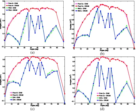
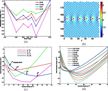
are represented by bigger yellow spheres, segregate on the first lowest energy sites. The blue and red spheres denote the copper atoms that lie on (002) and (001) planes respectively. Those structures whose head (tail) atom is replaced are marked as positive (negative) structure. (b) Illustration of theoretical (inside green shape) and actual (outside black shape) C structure. Two dislocations pile up at the bottom of C unit. (c) Illustration how disclination dipole strength affects the DSUM results, the red dot line is the grain boundary energy of Copper calculated from atomistic models. The blue rectangle line and the green triangle line are DSUM predictions with and without dipole strength modification respectively. ... 40 Figure 2.2: Dependence of energies of 〈100〉 symmetric tilt grain boundaries on the tilt angle for four

systems. Respectively: (a) Pb dopped Al; (b) Nb dopped Cu; (c) Zr dopped Zr and(d) Zr dopped Cu systems. The rectangle lines are computed directly from atomistic models with EAM potential, the solid circle lines are obtained from DSUM model. The red and purple lines correspond to pure metal system, the blue and green lines represent grain boundary energy of solute induced systems. ... 41 Figure 2.3: Stabilization effects shown by (a) Energies of different bond types of four alloy systems;

Σ17-530 grain boundary. (c/d) Dependence of grain boundary energy on area density of

impurities in different alloy systems / with different tilt angles. ... 42

Figure 2.4: Comparison between expansion obtained and full calculations of segregation energies for Cu-Zr alloy. Values denoted by triangles are obtained from Eq. (2-9) only, and the circles are computed under the approximation of Eq. (2-10). Data with circle are elevated by 0.1 eV intentionally so that two sets of date are distinguishable. ... 43

Figure 3.1: Demonstration of three stable states (A, B, C) during a simulation of grain boundary migration. State A is the initial state during the TPS calculation and the reaction coordinate is defined as the position of the grain boundary. ... 51

Figure 3.2: Tilt angle dependence of (a): Mobilities at 800K and (b): corresponding activation energies for STGBs of copper as listed in the Table 2.1. The dashed dots are the stationary GB energies as reported in Figure 2.2. ... 54

Figure 3.3: (a), initial and final position of atoms in Σ17-530 STGB, (b) y-component of displacement profile of atoms in (a) along z-direction. ... 56

Figure 3.4: Demonstration of activation energies computed by fitting temperature dependent GB mobility to different equations. The symbols are ensemble averaged MDS results, dashed lines are the fits using Eq. (3-1) and solid lines are the fits according to Eq. (3-7) ... 57

Figure 3.5: Correlation function and its linear fit for the Σ17-530 STGB at 600K. ... 59

Figure 3.6: Histogram plot of Σ17-530 STGB being at different stable states at t=5000fs. ... 60

Figure 4.1: Illustration of atomistic model used in the simulation. ... 66

Figure 4.2: Energy profile along RC for Σ12-320 with different systems sizes ... 67

Figure 4.3: Geometry characteristics of grain boundary sliding. ... 70

Figure 4.4: Comparison between barrier heights from NEB calculations and activation energies from Arrhenius law ... 72

Figure 5.1: Illustration of idea 1-D diffusion model for laminate Al – CuO thermite composite ... 82

Figure 5.2: Demonstration of using a model fitting method to interpret DSC curves. The solid line with cycles is the normalized DSC curve as a function of temperature. The insert are the model fitting curves based on various model functions listed in Table 5.4. ... 84

Figure 6.1: Illustration of sample geometries considered. Left: Laminate, Center: Cylinder, Right: Sphere. ... 92 Figure 6.2: Plots of the Zr/CuO data in Table 6.1. (A) Given as a Kissinger plot, i.e. Eq. (3-9). (B)

Plotted via Eq.(6-5). Diamonds, squares, triangles, circles and ×’s correspond to 1-5 bilayers, respectively ... 100 Figure 6.3: Plots of the Al/CuO data in Table 6.1. (A) Given as a Kissinger plot, i.e. Eq.(3-9). (B)

Plotted via Eq.(6-5). Diamonds, squares, triangles and circles correspond to 1-4 bilayers, respectively. ... 101 Figure 6.4: Natural logarithm of diffusion coefficient as a function of the inverse of the temperatures

times Boltzmann’s constant. The thick solid line is the diffusion coefficient predicted from the plot in Figure 2B over the temperature range at which the peak temperatures were measured. The thinner solid lines and the open diamonds are experimental data for self-diffusion of oxygen in Zr[152]–[156]; dashed and dotted lines correspond to experimental data for oxygen self-diffusion ZrO2 and in CuO, respectively[157]–[160].The line lengths correspond to

the temperature over which the measurements were taken. ... 104 Figure 6.5: DSC curves for a Zr-CuO nano- laminate for different numbers of bi-layers. Dotted lines

are experimental data; the solid lines are from Eq.(6-3). The curves are offset along the y axis for clarity. The points are used to determine the diffusion kinetics, while the dotted line represents the fit of Eq.(6-5) to the experimental data. ... 106 Figure 6.6 Peak shape calculated from Eq.(6-19) for different values of thermal conductance. ... 107 Figure 6.7: Plot of data from Table II. (a) Scaled according to Eq. (6-5). (b) Scaled according to Eq.

(6-17). ... 109 Figure 6.8: Plot of data from numerical DSC curves for laminar, cylindrical and spherical multilayer

systems scaled as given by Eq.(6-5). ... 110 Figure 7.1: Geometries of Al-CuO multiple layer nano-laminate modeled by continuum dynamics. (a)

Figure 7.2:Temperature profiles that demonstrates the different stages during joule heating and thermite reaction. (a) t=0.001s. (b) t=0.025s. (c) t=0.027s. The small time and large

temperature difference between panels (b) and (c) compared to those between panels (a) and (b) is consistent with the delay time and rapid reaction observed experimentally ... 122 Figure 7.3: Logarithm of time before initiation vs. pre-exponential component with Ea=150kJ/mol and

applied potential V1=0.1 V. ... 123

Figure 7.4: Dependence of reaction propagation speed on pre-exponential constant of Eq. (7-6)... 125 Figure 7.5: Dependence of reaction propagation speed on activation energy of Eq. (7-6). ... 125 Figure 7.6: The wire heating experiment. (a) The experimental setup, in which a Pt wire is embedded

in the top CuO layer, and Joule Heating is applied by applying constant electric potential on the two sides of the Pt wire. (b) The SEM image of the cross section of the final product. (c) The composition mesh of CuO in the final state in the simulation II. (d) The temperature profile before ignition.. ... 126 Figure 7.7: Comparison of DSC curve obtained from simulation (a) and from experiments (b). Note

that the units of x axis are Kelvin for (a) and Celsius for (b) respectively. ... 127 Figure 8.1: Sketch of the family tree for hyperthermia treatments in oncology ... 133 Figure 8.2: Demonstration of the relationship between SHR(tp), activation energy and diffusion

pre-exponent in nano energetic materials. The plot was made from numerical solution of 1-D diffusion equation with p=0.2 at the temperature 36.8°C and enthalpy of the reaction is 1kJ/g. ... 137 Figure 8.3: A design of nano-composite of maghemite coated nano thermite for hyperthermia

P

1,

G

Chapter 1 An Overview of the Computational Study of the Grain Boundary Structure , Energy and Mobility

1.1 Introduction

With the advent of high performance computers, computation and simulation

approaches are changing the way we learn, view, and study in material science. Yet the value of computation and simulation, as the third pillar of research, standing equally alongside theory and experiment, is still underappreciated. A very similar remark was made in the Presidential Information Technology Advisory Committee [1] report: “Universities...have not effectively recognized the strategic significance of computational science in either their

organizational structures or their research and educational planning.” This has been

especially true in the computational study of solids in materials science. There appear to be several reasons for this, the most evident one is that, even today, computational resources are limited compared to most of the problems encountered in the practical study of solids.

Grain boundaries, for example, are two-dimensional nonequilibrium defects in crystalline solids. It has been proven that many crystalline materials can be strengthened (known as Hall–Petch strengthening[2]) by introducing grain boundaries because grain boundaries can impede dislocations motion. In this view, materials with ultra-fine grains would have ultra-high strength. However, this is not true microstructures of nano crystalline material are often thermally unstable because grain boundaries are associated with positive free energy which means that their configurational entropies are smaller than their formation energies. Minimization of the free energy will drive grain boundaries to move, which is the dominating mechanism for grain growth during the annealing of metals. However, it has also been found first by molecular dynamics simulation[3], [4] and then confirmed by many

experimentalists[5]–[7] that solute segregates can stabilize grain boundaries and further make ultra-strong materials possible. From this example, we can see how complex the

1.2 Molecular Dynamics and Interatomic Potentials

Molecular dynamics is a straight-forward computational simulation in which the motion of atoms is followed and analyzed under different conditions[8]. The chief assumption in this technique is that atoms can be treated as classical particles so that their trajectories are calculated by numerically integrating classical Newton equations of motion for each atom. These equations of motion are coupled through the forces on the atoms. The interatomic forces which determine the dynamics of atoms are a key feature of a MDS. They are also typically the most computationally intensive part of the simulation. The forces on the atoms are derived from the negative gradient of the potential energy function (PEF) which is an empirical function for calculating the potential of the system given all atom positions. Conventionally PEF is split into one-body, two-body, three-body … terms:

𝑈(𝒓𝑁_{) = ∑ 𝑉} 1(𝒓𝑖) 𝑖

+ ∑ ∑ 𝑉₂(𝒓_𝑖, 𝒓_𝑗)

𝑗>𝑖 𝑖

+ ⋯ _(1-1)

And the interatomic forces:

𝑭𝑖 = ∇𝒓𝑖𝑈(𝒓𝑁) (1-2)

where 𝑟𝑖 refers to the position of the 𝑖𝑡ℎ atom; 𝑁 is the total number of atoms; 𝑈(𝒓𝑁) is the

PEF; 𝑉1(𝒓𝑖) is the one body potential which usually represents the interaction between the

𝑖𝑡ℎ _{atom and an externally applied potential field; 𝑉}

2(𝒓𝑖, 𝒓𝑗) is the two-body potential. It is

used to describe pair interactions such as the electrostatic, van der Waals or bond

interactions. Three body potential and higher order many body potentials are mostly seen in

Mathematical forms of PEF came in with great varieties, applicable in different situations. Even for the pair potential, a number of functional forms have been developed, such as Lennard-Jones potential, Morse potential and their countless derivatives[9]. Since this section is by no means a complete review of interatomic potentials, we refer the reader to other reviews[10]–[12] mentioned in the bibliography.

In practical MDS, the criteria being a good PEF is three fold: (i) accuracy: it should accurately reproduce some set of fitting data from experiments or quantum chemistry models such as density-functional theory; (ii) transferability: it should be also capable of producing physically-reasonable (if not accurate) energies for atomic configurations that are not considered in a given fitting database; (iii) efficiency: it should be computationally efficient so that MDS can: generate sufficient number of samples, contain sufficient number of atoms in the system, and perform for sufficient long time to minimize statistic errors and capture the relevant physics of a given problem.

Experience has demonstrated PEFs that find a compromise between accuracy,

transferability and efficiency are based on expressions that are derived from quantum

mechanical bonding principles. Potential of Embedded Atom Method (EAM) for metallic

system is such an example. Different from conventional pair potential which consider

interaction between to particles are not affected by the presence of other atoms, EAM add to

the PEF a cohesive energy term which describes the energy of embedding an atom into an

local electron gas provided by the neighboring atoms. More detailed description of EAM

potential can be found in the Chapter 2 and elsewhere[11], [13]–[15]. But see from the EAM

two reasons. First, it is many-body potential in which the metallic bond strength between two

atoms is coordinate dependent. This makes EAM an effective potential for pure metal

systems. Second, EAM is computationally efficient. By using pair terms for inter-atomic

repulsion and the electron density contributions to a given site, the evaluation of the EAM

scales as a pair potential despite the many-body aspect of the function that is introduced by

an embedding function. It is because of these advantages that EAM has found wide

application in the computational study of metals. Throughout this thesis, EAM potential or its

direct derivative, modified EAM[14], is used unless specified.

1.3 Basic Conceptions of Grain Boundaries

A grain boundary is an interface separating two crystals (grains) of the same crystal but of different orientations. Grain boundaries are planar defects because the discrepancy of crystal orientations across the grain boundaries brings in misfit energy and stresses. Despite grain boundaries being recognized and studied for centuries, they are still among the least understood structures in materials science because of their extremely complex structures.

inclination of grain boundary plane but variable translation vector were energy minimized by molecular dynamics simulation using an embedded atom model (EAM) potential so that the minimum energy configuration can be found. Their results showed very good agreement with high-resolution transmission electron microscopy images of experimental grain boundary structures.

To simplify the description of grain boundary crystallography, a number of variables or terminologies are frequently used in the literature. Some of them are summarized below:

Tilt and twist grain boundaries

(a)

(b)

Figure 1.1: Illustration of a pure tilt grain boundary (a) and a pure twist grain boundary (b).

Low and high angle grain boundaries

Grain boundaries with small (usually 𝜃 ≤ 15 °) misorientation between adjacent grains are called low angle grain boundaries; accordingly, those who have large

misorientation are called high angle grain boundaries. This way of classifying grain boundaries is not precise and the dividing line often varies from one research paper to another. However, it is an important concept that is frequently seen in the literature. This is because low angle grain boundaries can often be approximated as an array of dislocations (edge dislocations for tilt, and twist dislocations for twist grain boundaries), but this approximation is invalid in the high angle region.

edge dislocations. But in high tilt angle cases, the edge dislocations are so close that the dislocation cores begin to overlap and the definition of the Burger’s vector become unclear.

Figure 1.2: Atomic configurations of symmetric tilt angle grain boundaries from low to high

misorientation. The bottom angular lines show the half of the misorientation angle, i.e. θ/2. From left to right, θ/2 values are 3.02°, 6.04°, 18.44°, 23.20° and 26.57° respectively.

Based on the idea that low angle grain boundaries can be represented by an array of dislocations, Read and Shockley developed the expression for the energies of low angle grain boundaries

𝐸_𝑔𝑏 = 𝜃(𝐴 − 𝐵 ln 𝜃) (1-3)

Figure 1.3 demonstrates the grain boundary energy prediction based on Eq. (1-3) and from molecular dynamics simulation with an EAM potential[11]. The results from the Read and Shockley formula and full atomistic calculation are in good agreement in the low angle region. In high angle region, the Read and Shockley formula predicts an energy decrease for high-angle grain boundaries but in the EAM calculation, the energies remain almost constant for the high angle grain boundaries.

Coincidence Site Lattice (CSL) and the Reciprocal Density

Although the expression “CSL theory” is frequently used in the research papers, CSL itself is not a theory but an imaginary lattice formed by the coincide sites of two regular lattices with special misorientation angles. For instance, shown in the Figure 1.4 is a demonstration of a Σ5 structure. The blue and green circles are the crystal structure (simple cubic) of the same structure. The lattice formed by big red circles, i.e. coincide sites is known as the CSL.Σ is called the reciprocal density; it is defined as a half of the number of atoms included in one CSL cell. In this example, four green, four blue and 8 coinciding vertices (shared by 4 CSL cells) are included in one CSL cell. Therefore the Σ value for the structure is (4+4+4×1/4)/2=5.

1.4 Coarse Grained Representation of Equilibrium Grain Boundaries

Serves as supplementary for Chapter 2, this section will present an historical review of coarse grained models of grain boundaries. As mentioned in the previous section, grain boundaries are often treated as an array of dislocations. This treatment can be traced back to 1950 when the well-known relationship between grain boundary energy and misorientation angle, i.e. Eq. (3-9), was derived[17]. A similar express was also derived by Nabarro in 1952[18] by integrating the elastic forces on each dislocation from its actual position to

infinite distances. In these two cases, grain boundaries were represented by a finite number of equally spaced dislocations. However, in 1953, James[19] pointed out that a grain boundary is better represented by infinite number of dislocations. The stress fields of the two resemble one another only at the distance from the wall nearer than the dislocation spacing in the wall. Despite the huge success of the dislocation wall model for grain boundaries in the 1950s, researchers found difficulties fitting this model to high angle grain boundaries. In 1960, James[20] examined the dislocation wall model for high angle tilt grain boundaries and declared that if the interactions of cores of the dislocations are taken into consideration, a dislocation wall model can well represent grain boundaries even in the high tilt angle region. Another effort in extending the dislocation wall model to the high angle grain boundaries is from Brandon, who proved that the dislocation wall model is compatible with coincidence lattice model in the high-angle region[21].

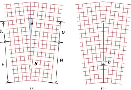
disclination into the material. In 1972, Li[23] proposed that grain boundaries should be

considered as being made of disclinations instead of dislocations because a grain boundary is a rotational defect and so are disclinations (dislocations are translational defects). Moreover, similar to the conclusion by Eshelby[22], Li discovered that the energy of a symmetric tilt grain boundary (STGB) can be computed easier using the disclination model than the dislocation model. In Li’s paper[23], STGBs are made of equally spaced (spacing H) disclination dipoles whose strengths are 𝜔 as shown in the Figure 1.5.

(a) (b)

Li further assumed that each disclination can be viewed as one low angle infinite dislocation wall consisting of M edge dislocations of Burger’s vector 𝑏′_{. Further some}

imaginary dislocations with Burger’s vector of zero were added to this picture so that the geometry and the number of dislocations have a relationship 𝑀 𝑁⁄ = 2𝐿 𝐻⁄ , where 2𝐿 is the height of the disclination dipole as illustrated in Figure 1.5. The energy of this simple STGB can then be expressed as the sum of all disclinations plus the elastic energies between every two disclinations.

𝐸𝑔𝑏 =

𝜇𝑏′

4𝜋(1 − 𝜈)𝐻[𝑀 ln 2𝜋𝑟₀

𝑒𝐻 + 2 ∑ (𝑀 − 𝐼) ln (2 sin 𝐼𝜋

𝑁)

𝑀−1

𝐼=0

] (1-4)

where μ and ν are shear modulus and Poisson ratio of the investigated material.

Shortly after Eq. (1-4) was derived, Shih and Li[24] extended the idea of disclination models to the grain boundaries that consist of alternate disclination dipoles of 𝜔₁ with height 2𝐿₁ and 𝜔₂ with height 2𝐿₂. Moreover he rewrote the strain energy part the Eq. (1-4) by replacing the summation with integration to make it more precise and independent of imaginary Burger’s vectors of 𝑏′. The elastic strain energy of the STGB now is

𝐸𝑒𝑙 =

𝜇Δ𝜔2

8𝜋(1 − 𝜈) 𝐻

4𝜋2𝑓(𝜆1) (1-5)

where Δ𝜔 = |𝜔₁ − 𝜔₂| and function 𝑓(𝜆₁) is given in Eq. (2-3).

Despite the huge success of Eq. (1-4) and Eq.(1-5), they are still continuum

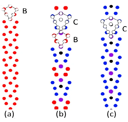
work Sutton and Vitek[25] found that some atomistic structural patterns show up repeatedly in the grain boundaries. For example, illustrated in Figure 1.6 are the atomic configurations of the last three grain boundaries in Figure 1.2. It can be seen clearly that Figure 1.6a and Figure 1.6c consist of monotonic repeating structures and historically, they are defined as “B” and “C” structural units, respectively. Figure 1.6b, on the other hand, is made of alternating “B” and “C” structural units. Grain boundaries that are composed of contiguous sequences of one type of fundamental structural units are called “favored boundaries” which usually have low reciprocal density, i.e. Σ value, of coincidence lattice and low strain energy.

In 1986, Wang and Vitek[26] developed a way to compute grain boundary energies based on the structural units model and the dislocation model for grain boundaries. In their paper[26], the total energy of a grain boundary consists of the energy of a reference structure, the core energy and the elastic energy:

𝐸_𝑔𝑏 = 𝛾_𝛼+1

𝑑[𝐸𝑐 + 𝜇𝑏2ln 𝑒𝑏

2𝜋𝑟₀] (1-6)

where 𝑑 is the average spacing of the dislocations and 𝑏 the magnitude of their Burger’s vectors. 𝛾𝛼 is the reference energy and were calculated from atomistic models of the favored

grain boundaries. For instance, 𝛾_𝐵 and 𝛾_𝐶 are the energies of the grain boundaries shown in Figure 1.6a and Figure 1.6c respectively. 𝐸_𝑐 ≈ 𝛾_𝛼𝛽⁄2 , is the core energy and 𝛾_𝛼𝛽 is the energy of the boundary that has an equal number of 𝛼 and 𝛽 units. For instance, 𝛾𝐵𝐶 is the

energy of the grain boundary (b) in Figure 1.6.

Formula (1-4) was based on the dislocation model and it involves many unnecessary approximations, such as 𝐸𝑐 ≈ 𝛾𝛼𝛽⁄2. In 1989, Gertsman et. al. proposed a disclination

1.5 Approaches to Compute Grain Boundary Mobilities

Grain boundary motion is an important aspect to many recovery processes such as grain growth during recrystallization post cold work hardening. Despite many efforts aimed at understanding the details of grain boundary migration, the complexity of the atom

dynamics associated with grain boundary motion, and how these dynamics are coupled to internal stresses and external applied strains, makes it one of the major unresolved problems in materials science [32].

During grain growth different grain boundaries can behave quite differently. In most annealing experiments, grain growth represents an average behavior of many types of grain boundaries. This limits the ability to understand grain boundary dynamics of one specific interface type. Even in bi-crystal experiments [33], [34] it is still a formidable task to study migration of single grain boundaries throughout a large range of misorientation angles. In contrast, molecular dynamics simulation can provide unique insight and predicted properties of specific grain boundaries that complement experimental capabilities [35].

angle is not a typical feature of experimental or atomistic simulation results. For higher tilt angles, assuming that grain boundary motion is closely related to atom diffusion leads to the Burke-Turnbull expression for grain boundary velocity of the form

𝑣 = Ω

𝑎2 [η𝑒− 𝑄𝑘𝑇− 𝜂𝑒 𝑄+𝑝Ω

𝑘𝑇 _] (1-7)

where Ω is the volume per atom, a is the lattice spacing, η is an attempt frequency, Q is an activation energy, k is Boltzmann’s constant, T is temperature, and p is pressure. In the limit that pΩ >> kT, velocity and pressure are proportional to one another with proportionality constant (i.e. mobility):

𝑀 =𝜂𝑎4 𝑘𝑇 𝑒

− 𝑄_{𝑘𝑇 (1-8)}

In this expression the mobility is an activated process, but is independent of tilt angle. Based on both experimental studies and molecular dynamics simulation, grain boundary mobilities depend on many factors, but with a dependence that is not well

understood. There are, however, several trends that have become apparent. First, high angle grain boundaries tend to be more mobile than low angle structures, a trend that in general appears valid for both twist and tilt structures. [39]. In addition, in contrast to the analytic theory mentioned above the mobility of low angle grain boundaries tend to increase with increasing misorientation angle in a power law relationship M = kθα[39]

different for planar and curved grain boundaries and highly sensitive to impurity and vacancy concentrations. [41].

To help establish relations between structure and mobility for individual grain boundaries, Foiles and co-workers used molecular dynamics with an artificial driving force method mentioned above [42] to calculate energies and mobilities for a total of 388 grain boundaries in nickel. These interfaces included 〈111〉, 〈100〉 twist, and 〈110〉, 〈111〉, 〈100〉 symmetric tilt and coherent twin grain boundaries[35]. They reported that over 25% of the grain boundaries migrate via a mechanism that couples shear stress to motion; this included a majority of the non- Σ3 structures that had the highest mobilities. Of the remaining structures, the incoherent Σ3 twins had an anomalously high mobility, while some other boundaries (e.g. all of the <111> twist boundaries) remained static on the time scale of the simulations. Thermal activation energies were also found to vary widely, with some migration mechanisms not having any measured activation barriers. They also reported thermal roughening of the grain boundaries, with substantial increases in grain boundary mobility above the roughening temperatures for each boundary. Despite the wide range of different properties for the different structures, no correlations were discovered between mobility and scalar quantities such as misorientation angle, grain boundary energy, Σ value or excess volume.

The definition of grain boundary mobility implies a linear relationship between grain boundary normal velocity and driving force. Both analytic theory (c.f. Eq.(1-7)) and

boundary velocity is proportional to driving force (v_GB ∝ P ) for twist grain boundary motion, but is nonlinear (v_GB ∝ P2_{) for tilt grain boundaries. This result is ascribed to local}

interactions between the grain boundary and nearby dislocations. Another tentative explanation has been proposed by Zhang et al [44] who attributed the nonlinearity to an increase in effective activation barrier with increasing applied driving force.

A mechanism based on Eq.(3) was proposed by Zhou and Mohles [43], who suggested that the approximation leading to Eq.(4) is invalid for the high forces needed to observe grain boundary motion in MDS. They suggested that the low driving force limit can be achieved by extrapolating data from high driving force simulations. Based on this idea, Zhou and Mohles determined misorientation-angle-dependent grain boundary mobilities and migration

activation energies by molecular dynamics simulation using the artificial driving force method [42]. In their work, a series of flat twist 〈110〉 grain boundaries with various Σ values and misorientations were investigated. The resultant mobilities of small (≤ 25o_{) and large}

misorientation grain boundaries are about 1 × 10−9_m4_J−1_s−1 _{and 1 × 10}−8_m4_J−1_s−1

respectively.

One way of avoiding the nonlinearity resulting from a high driving force is to perform equilibrium molecular dynamics simulation and obtain the mobility according to the

similar to those extracted from molecular dynamics simulation with a curvature driving force.

Similar to grain boundary mobility, there is no simple rule to determine activation energies of grain boundary migration because the energies depend on too many variables such as grain boundary type, impurity concentration, and shape. Activation energies computed from molecular dynamics simulation, for example, are often lower than those determined from experiment, [43], [46]. One contributing factor to this observation is likely the presence of impurities in the experimental systems that are not present in the simulations [35].

A distinct transition in activation energy between low angle and high angle grain boundaries, irrespective of planar or curved type, at approximately the same misorientation was detected numerically [43] and experimentally [47]. The transition angle measured is about 15° for both 〈110〉 twist [43] _{and 〈100〉 twist boundaries,} [46]_{, 14.1° for 〈111〉 symmetric tilt} boundaries [47], 8.6° for 〈100〉 symmetric tilt boundaries [36] and 13.6° for 〈112〉 symmetric tilt [48] grain boundaries. The first two transition angles were determined from molecular dynamics simulation while the latter three were measured experimentally. The agreement suggests that molecular dynamics simulation is able to capture the important aspects of this transition.

In a recent experiment by Ruper et al., it was observed that grain boundary migration in nanocrystalline aluminum thin films is governed by shear stresses that produce distortion work rather than normal stresses assumed in conventional theory. [49]. Shear stress as driving force for grain boundary migration has also been reported in other experimental studies [32], [36], [48]

studies [50], [51]. By performing molecular dynamics simulation for symmetric 〈100〉 tilt grain boundary systems in copper, Cahn et al. confirmed that the normal motion of planer grain boundaries can be driven by shear stress and the ratio of normal to tangential translation of a grain boundary is a constant independent of temperature or of the magnitude of the applied shear stress. In a study by Olmsted et al.[35], they found that even under a normal driving force significant shear can be built up during normal motion of planer grain boundaries. They further claimed that the normal, diffusion controlled mechanism exists in all grain

boundaries, but it is often overshadowed by the fast shear coupled mechanism if the latter is allowed geometrically, for instance if lateral translation is unconstrained.

1.6 Overview of Chapters 2 – 4

In Chapter 2, considerable efforts will be placed on developing multi-scale, coarse grained models of nanostructured materials. Multiscale modeling describes a wide range of computational activities that are aimed at describing phenomenon of materials at a fine scale level by modeling or simulating at a coarser scale. More specifically, in conventional

The third chapter is dedicated to computing mobilities of symmetric tilt grain boundaries for face-centered cubic copper and detecting grain boundary migration

mechanisms. A limitation of applying computation and simulation tools in material science is that most available methods have narrow and strict application ranges. Scholars must be very aware of the approximations made and how much the error will be brought in before making use of one method. What is even worse is that limits on the applicability of those

computation and simulation methods are undefined for a wide range of methods. This circumstance is even worse when it comes to computer simulation of non-equilibrium processes such as grain boundary migration because many competing mechanisms are in presence simultaneously. Conventional molecular dynamics simulation of grain boundary migration tends to predict an abnormally high mobility and low activation energy for grain boundary motion. In Chapter 3, we first follow the conventional way of computing grain boundary mobilities using molecular dynamics and then demonstrate how the resulting mobilities and activation energies can be better interpreted if various migration mechanism are taken into consideration.

In the annealing process of multi-crystalline materials, dislocation gliding and climbing are generally considered as the two most important atomistic mechanisms.

However, occurrences of these two events are not uniformly distributed during the recovery phase of an actual material because climbing is often overshadowed by gliding if the

very poor despite the fact that computational studies have been being carried on for decades. One objective of Chapter 4 is to present in depth discussions on characterizing and

Chapter 2 Solute Segregation Energy and Grain Boundary Energy Calculation Based On Disclination Structural Units Model and Perturbation Methods

It has been shown in many experiments that solute atoms segregate to and can

stabilize grain boundaries in dilute alloys due to the decrease of grain boundary energies after segregation. In this chapter, we propose a few computational tools for studying the

stabilization effects of solute atoms in pure metal grain boundary systems from an energy perspective. Tools are (i) a quick way to locate favorite segregation sites for atomistic models, (ii) a semi-analytical formula to compute the grain boundary energy for low sigma grain boundaries with dilute solute segregate and (iii) a highly-efficient method to calculate the segregation energy of solute atoms at all possible lattice sites using perturbation

techniques together with an extended disclination structural units model.

2.1 Introduction

The investigation of grain boundary structure and mechanical properties of dilute alloy systems is of substantial scientific and technological interest due to its application in studying solute segregation [52] and grain boundary stabilization [53][5]. For instance, grain boundary mobility measured in bicrystal systems has been found to be sensitive to impurity

concentrations[54]. Even extremely small quantities of tellurium in high purity copper[55] and silver in high purity lead[56] have pronounced effect on their recrystallization processes. These effects are widely agreed as a result of solute atoms concentrating on the grain

boundaries and in bulk metals can be as high as 10,000[52]. To investigate the effects of solute atoms on the mechanical behavior of grain boundary systems, one must firstly be able to compute the grain boundary energies with solute atoms at various lattice sites and moving the solute atoms from those sites to the grain boundary.

Conventionally, atom structures and molecular dynamics (MD) or first principle calculations are required to compute these energies. However both atom models building and micro scale simulations require lots of efforts to complete. A practical challenge is how to compute these energies without building atom level models or perform exhaustive micro scale simulations. For simple pure metal systems with low Σ boundaries, it is a solved problem. It has been shown that grain boundary energy of pure metal system, can be computed from the disclination structural units model (DSUM) [23], [26], [29] which is a

macroscopic model based on linear elasticity theory that does not require any information of atom level structures (See Chapter 1 for details). However, when solute atoms are included in the system, the case becomes complicated because the chemical interactions have been changed around the solute atoms but linear elasticity does not taken these changes into consideration. Moreover, the energy change of introducing a solute atom is position dependent and is almost impossible to be computed without the knowledge of the atomic structure of the system. In this chapter, we propose that energy of a grain boundary with solute segregates can be calculated quickly for the following two cases.

enormous, the configurations that produce the lowest grain boundary energies are relatively fixed.

2. The dilute solute case. In this case, interactions between solute atoms are considered weak compared to the energy of introducing these solute atoms. Then overall

potential energy can be treated as a function of segregate positions only.

In the following text, a brief review of the background knowledge for computations of both cases is given first. This section contains three parts. First, the formulation of the DSUM theory is presented. Methods to categorize and compute solute segregation energy levels are then introduced. In the third part, we report a method to quickly compute the energy change of introducing single solute atoms at arbitrary lattice sites with minimum knowledge of atom structures and computational effort. In the following section, 30

symmetrical tilt angle grain boundaries with various misorientation angles were built for four alloy systems. All-atom molecular dynamics simulations were performed firstly to obtain the stabilization energies and grain boundary energies. Then those values were compared to the respective values computed from the formulas proposed in the last section to confirm the validity of our methods.

2.2 Theory

high Σ grain boundaries. Here Σ is the reciprocal density of coincidence sites. The DSUM has proven to lead to reasonable energy estimates for several pure metal systems [25], [27], [59] and a few covalent materials such as silicon and diamond [29]. Recently, Purohit, et. al successfully applied the DSUM to a Pb-Al alloy system[28]. However, later calculation suggested that the method in [28] is not extensible to other alloy systems. In this work, we extend the power of both atomistic modeling and DSUM method to solute-stabilized systems.

The DSUM describes a grain boundary with misorientation angle 𝜃 as a linear combination of alternating segments of two specific disclination units whose misorientation angles are 𝜃1, 𝜃2 respectively. The elastic energy of the grain boundary is therefore an

expression of partial disclination dipole strength 𝜔 = |𝜃₁− 𝜃₂|, where 𝜃 is then angle of structural units shown

𝐸_𝐺𝐵𝑝𝑢𝑟𝑒 = 𝑛1𝑑1𝜀1+ 𝑛2𝑑2𝜀2

𝐻 + 𝐸𝑒𝑙𝑎𝑠𝑡𝑖𝑐+ 𝛼

𝐺𝑎₀2_𝜔2_𝑛

2𝜋3_{(1 − 𝜈)𝐻} (2-1)

with

𝐸𝑒𝑙𝑎𝑠𝑡𝑖𝑐= 𝑛𝐺𝜔 2_𝐻

32𝜋3_{(1 − 𝜈)}{𝑓(𝑛𝜆)

+ ∑ ∑ [𝑓(𝑦̃𝑗− 𝑦̃𝑖+ 𝜆) − 2𝑓(𝑦̃𝑗− 𝑦̃𝑖) + 𝑓(𝑦̃𝑗− 𝑦̃𝑖− 𝜆)] 𝑛

𝑗=𝑖+1 𝑛−1

𝑖=1

}

(2-2)

where 𝜆 = 𝜋𝑑₂/𝐻, 𝑦̃_𝑖 = 𝜋𝑦_𝑖/𝐻,y_i are the coordination of disclination dipoles., 𝑛_𝑖, 𝑑_𝑖, 𝜀_𝑖 are, respectively, the number, length, and energies of specific disclination units and 𝐻 = 𝑛₁𝑑₁+ 𝑛2𝑑2 is the period of the grain boundary.

dipole wall (DDW) which is the sum of the interaction energies composing disclination structural units. Function f(t) is given by

f(t) = −16 ∫ (t − v) ln[2 sin(v)] dvt

0

(2-3)

To extend Eq.(2-1) ~ (2-3) to dilute alloy system, we added one term to the right side of Eq. (2-1)

Ẽ_GBalloy = Ẽ_GBpure+ Ẽ_sub (2-4)

where the term 𝐸̃_𝑠𝑢𝑏 is called the substitution energy, it measures the energy change of replacing a metal atom with a solute atom in the grain boundary system. The tilde symbol denotes that the energies are obtained from fully relaxed atom structures at O K. The substitution energy varies from site to site due to the lattice disordering near the grain boundaries.

Generally speaking solute atoms tend to occupy those lattice sites near or in the grain boundary. This behavior is known as solute segregation. To determine the energetically preferred segregation sites for solute atoms, we need to find a way to estimate the

substitution energy with respect to each lattice site in an atomistic model. In our work, this calculation is done by modifying the EAM formula. In the framework of the EAM potential, the energy of atom 𝑖 is given by

𝐸_𝑖 = 𝐹_𝛼[∑ 𝜌_𝛽(𝑟_𝑖𝑗)

𝑖≠𝑗

] +1

2∑ 𝜙𝛼𝛽(𝑟𝑖𝑗)

𝑖≠𝑗 (2-5)

potential function, and 𝛼, 𝛽 are the atom types of atom 𝑖 and 𝑗. Here we define an inplace substitutional energy(𝐸𝑖𝑠𝑒) as the energy difference when the atom at site 𝑖 with type 𝛼 is

replaced by new atom 𝛽 without atomic structure relaxation.. The inplace substitutional energy based on Eq. (2-4) can be expressed as

𝐸_𝑖𝑖𝑠𝑒= ∑𝑑𝐹𝜏

𝑑𝜌[𝜌𝛼(𝑟𝑖𝑗) − 𝜌𝛽(𝑟𝑖𝑗)]

𝑗≠𝑖

+ ∑ 𝛿𝐹𝛼,𝛽[𝜌𝛼(𝑟𝑖𝑗)] 𝑗≠𝑖

+ ∑ 𝛿𝜙𝛼,𝛽(𝑟𝑖𝑗)

𝑗≠𝑖 (2-6)

where 𝛿𝐹_𝛼,𝛽 ≡ 𝐹_𝛼− 𝐹_𝛽, and 𝛿𝜙_𝛼,𝛽 = 𝜙_𝛼𝜏− 𝜙_𝛽𝜏 are the functional differences and 𝜏 is the atom type of the atom at site 𝑗. We have implemented this functionality as a plugin in the LAMMPS molecular simulation code[60]. Eq.(2-6) is also applicable to other analytic potentials, for example, pairwise additive potentials (which are a special case of the EAM).

This energy is different from the substitution energy in Eq. (2-4). From a macroscopic viewpoint, the substitution energy has two contributions. One is from the chemical

environment change brought by introducing a segregate atom. In this article we refer to the in-place substitution energy as the chemical contribution. The elastic contribution comes from the structural relaxation. To calculate the true substitution energy, the in-place

substitute structure must be fully relaxed to achieve a stable structure. The energy decrease in the structure optimization step is given in Eq. (2-9) and discussed in more detail below.

𝐸̃𝑠𝑢𝑏 =

𝛿𝜀 𝑑1+ 𝑑2 =

𝜀₁₋₂− 𝜀₁ − 𝜀₂

𝑑1+ 𝑑2 (2-7)

The idea behind Eq. (2-7) is taking the all unit 1, unit 2 and the solute atoms in between combined as a new structural unit and taking into account the energy difference between the new unit 𝜀₁₋₂ and the two basic units, i.e. 𝜀₁ and 𝜀₂. This idea is very straight forward, and can be extended easily to other substitution sites. In the next section, Eq. (2-7) is tested and found to be valid for substitution sites with different energies.

Eq. (2-7)is limited to only a few special substitution sites. To compute substitution energies for arbitrary lattice sites, we propose a threefold expansion method:

1. Compute the grain boundary energy of a pure metal system (𝐸_𝐺𝐵𝑝𝑢𝑟𝑒) using the DSUM techniques given in Eq. (2-1).

2. Compute the in-place substitution energy (𝐸_𝑖𝑖𝑠𝑒) according to Eq. (2-6). 3. Compute the energy change (𝛿𝐸_𝑖𝑒𝑙) during structural relaxation of the in-place

substituted lattice using Eq.(2-8).

The energy change measured in step 3 is denoted by 𝛿𝐸_𝑖𝑒𝑙 _{because it is considered as the}

elastic contribution to the substitution energy as discussed earlier. In the framework of pair potential, the elastic energy change of the simplest case in which one metal atom at position 𝒓_𝑖 is replaced by a solute atom can be expressed as

𝛿𝐸_𝑖𝑒𝑙 ≡ 𝐸̃_𝑀𝑆𝑡𝑜𝑡_{− 𝐸} 𝑀𝑆𝑡𝑜𝑡

= ∑ [𝜙(𝒓̃_𝑘𝑗) − 𝜙(𝒓_𝑘𝑗)]

𝑘>𝑗,𝑘≠𝑖

+ ∑[𝜓(𝒓̃_𝑘𝑖) − 𝜓(𝒓_𝑘𝑖)]

𝑘≠𝑖

≈ ∑[𝜓(𝒓̃_𝑘𝑖) − 𝜓(𝒓𝑘𝑖)] 𝑘≠𝑖

≈ − ∑ 𝑭𝑘𝑖⋅ 𝛿𝒓𝑘𝑖 𝑘≠𝑖

where 𝐸̃_𝑀𝑆𝑡𝑜𝑡 _{and 𝐸}

𝑀𝑆𝑡𝑜𝑡 are the total potential energies of a metal system with one solute atom at

position 𝒓𝑖 before and after structural relaxation, the subscript 𝑀𝑆 means that the system

contains both metal(M) and solute(S) atoms, 𝜙 and 𝜓 are the pairwise potential functions describing metal-metal and metal-solute interactions respectively, 𝑭_𝑘𝑖 is the force on atom 𝑖 resulting from atom 𝑘, and 𝒓_𝑘𝑖 ≡ 𝒓_𝑘− 𝒓_𝑖 is the position vector between atoms 𝑘 and 𝑖. The right side of Eq. (2-8)is linked to the virial stress tensor[61] in the following fashion:

𝜎̃_𝑀𝑆𝑚_(𝒓

𝑖) − 𝜎𝑀𝑆𝑚(𝒓𝑖) = − ∑[𝑭̃𝑘𝑖⋅ 𝒓̃𝑘𝑖− 𝑭𝑘𝑖 ⋅ 𝒓𝑘𝑖] 𝑘≠𝑖

≈ 𝛿𝐸_𝑖𝑒𝑙_{+ 𝐶} 𝑒𝑙

(2-9) In Eq. (2-9), 𝜎𝑚 _{≡ −(𝜎}

𝑥𝑥+ 𝜎𝑦𝑦+ 𝜎𝑧𝑧) is the mean norm component of the virial stress

tensor. In elasticity theory, 𝜎𝑚 _{= 𝑃𝑉 where 𝑃 is the pressure of a solid body and 𝑉 is its}

volume. Therefore Eq. (2-9) is straightforward from a macroscopic viewpoint: 𝛿𝐸𝑒𝑙 ₌

∫ 𝑃𝑑𝑉 ≈ 𝛿(𝑃𝑉) − 𝑉𝛿𝑃. In Eq. (2-9), the assumption is made that 𝑉𝛿𝑃 is less position dependent than is 𝛿𝐸_𝑖𝑒𝑙 _{and thus can be treated as a constant. This validity of this assumption}

is confirmed below using fully atomistic simulations.

The reason of relating the elastic energy to the stress field is because in principle energy is not additive but stress field components are. This is an important property for DSUM based methods. It allows us to express the overall stress field of a complex structure as a linear superposition of the stress fields of a few composing units. Mathematically, it is given as

𝜎̂_𝑀𝑆𝑚_(𝒓

𝑖) ≈ 𝜎̂𝑀𝑆𝑚(𝒓𝑖) ≡ ∑ 𝜎̃𝜇,𝑀𝑆𝑚 (𝒓𝑖 − 𝒓𝜇)

where 𝜇=1 or 2 has the same meaning as the subscript used in Eq. (2-1). The hatted symbols differentiate the interpolated values from values determined from molecular simulation.

2.3 Experiment

Equations (2-6) and (2-7) yield the most likely substitution sites and give the corresponding grain boundary energies. Eq. (2-9)and (2-10) provide a way to compute substitution energy at arbitrary lattice site. To probe the accuracy of these formulas, thirty 〈001〉 symmetric tilt angle grain boundary structures have been built and tested; their

structural information in terms of basic structural units are listed in Table 2.1.

Simulations of 〈001〉 tilt grain boundaries in Table 2.1 are carried out using an embedded atom potential for four alloy systems, lead segregated aluminum (Al-Pb),

zirconium segregated aluminum (Al-Zr), niobium segregated copper (Cu-Nb) and zirconium segregated copper (Cu-Zr). The EAM calculations are performed LAMMPS, a Sandia-based parallel MD code[60].

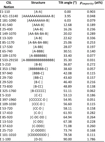
Table 2.1: 〈100〉 Symmetric tilt grain boundaries with impurities segregating at the first lowest energy sites; the term “alloy” means the solute induced system. The dash symbol “-“ in the Structure column is used to denote the site that connects two basic structural units and is substituted by impurity atoms. For instance, an B-C structure is equal to a combination of B+C- structure shown in Figure 2.1 (a).

CSL Notion

Structure Tilt angle (°) 𝝆𝒊𝒎𝒑𝒖𝒓𝒊𝒕𝒚 (at%)

Σ1-110 |A-A| 0.00 0.903

Σ 421-15140 |AAAAAAAAAAAAA-B| 3.95 0.048

Σ 181-1090 |AAAAAAAA-B| 6.03 0.079

Σ 41-540 |AAA-B| 12.68 0.189

Σ 25-430 |AA-B| 16.26 0.236

Σ 149-1070 |AA-BA-BA-B| 20.02 0.289

Σ 13-320 |A-B| 22.62 0.336

Σ 85-1170 |A-BA-BA-BB| 25.06 0.253

Σ 17-530 |A-BB| 28.07 0.197

Σ 65-740 |A-BBB| 30.51 0.140

Σ 109-1370 |A-BBBBBB| 33.40 0.077

Σ 533-29150 |A-BBBBBBBBBBBBBB| 35.30 0.031

Σ 5-210 |B-B| 36.87 0.272

Σ 353-1780 |BBBBBBB-C| 38.60 0.057

Σ 97-940 |BBB-C| 42.08 0.115

Σ 29-730 |BB-C| 43.60 0.157

Σ 29-520 |B-C | 46.40 0.216

Σ 73-830 |B-CC| 48.89 0.138

Σ 325-1760 |B-CCCCC| 51.11 0.062

Σ 5-310 |C-C| 53.13 0.186

Σ 397-1960 |CCCCCC-D | 54.95 0.051

Σ 109-1030 |CCC-D | 56.60 0.115

Σ 53-720 |CC-D | 58.11 0.158

Σ 17-410 |C-D | 61.93 0.282

Σ 85-920 |C-DC-DD | 64.94 0.264

Σ 13-510 |C-DD| 67.38 0.228

Σ 37-610 |C-DDD| 71.08 0.260

Σ 25-710 |C-DDDD| 73.74 0.168

Σ 101-1010 |CDDDDDDD | 78.58 0.111

The tilt axis is along the 𝑥 direction and the normal vector of each grain interface is along the 𝑧 axis. Each atomistic model contains a total of between 54648 and 100416 atoms and was fully relaxed using a conjugate gradient energy minimization algorithm. EAM potentials of Al-Zr, Cu-Nb and Cu-Zr systems are taken from the work of Sheng et al[62][15] , and that of Al-Pb system is from Landa’s work[63]. Those are highly optimized EAM

potentials designed for simulating alloy structures and mechanical properties at any

temperature. It predicts alloy structure in a reasonable agreement with experimental data. At zero temperature, the potentials predict perfect FCC structures whose lattice constants match first principle calculations.

Equilibrium relaxed structures at zero temperature are then found by minimizing the total internal energy with respect to all atomic positions. Further we resize the

dimensions of the simulation box to ensure that the total pressure of the block is zero (e.g. no artificial inner stresses are introduced). Grain boundary energies of both pure metal and alloy systems are computed and shown in the Figure 2.2.

2.4 Results and Discussion

Evaluating Eqs.(2-1) -(2-4) requires the energies of basic structural units A, B, C, D and the boding energies defined in Eq.(2-10). Because the basic units A and D are unit cells of perfect FCC lattice, 𝜀_𝐴 = 𝜀_𝐷 = 0 𝐽 ⋅ 𝑚−2_{. The energies of the basic units B and C are}

determined from EAM results of model Σ5 − 210 and Σ5 − 310 grain boundary structures We found for the Al-Pb system 𝜀_𝐵𝐴𝑙 _{= 0.443 𝐽 ⋅ 𝑚}−2 _{and 𝜀}

𝐶𝐴𝑙 = 0.451 𝐽 ⋅ 𝑚−2. Those values

are a little different for Al-Zr system,:𝜀_𝐵𝐴𝑙 _{= 0.489 𝐽 ⋅ 𝑚}−2 _{and 𝜀}

𝐶𝐴𝑙 = 0.487 𝐽 ⋅ 𝑚−2. In

principle these values should be equal since they all are computed from pure aluminum systems. However the disparity is understandable because they are calculated based with different EAM potentials. Similarly, in pure copper, the energies of the basic units are 𝜀_𝐵𝐶𝑢 _{= 0.862𝐽 ⋅ 𝑚}−2_{, 𝜀}

𝐵𝐶𝑢 = 0.830𝐽 ⋅ 𝑚−2 for the Cu-Nb system and 𝜀𝐵𝐶𝑢 = 0.834𝐽 ⋅ 𝑚−2,

𝜀_𝐵𝐶𝑢 _{= 0.807𝐽 ⋅ 𝑚}−2 _{for the Cu-Zr system, respectively.}

According to Eq. (2-4) both grain boundary energies of pure metal systems and impurity induced systems are calculated using EAM potentials; bond energies are then found as the difference of the two according to Eq. (2-10). Because the bond energies are most likely negative, they are the reason why grain boundaries are stabilized after solute atoms been introduced, they are also called the stabilization energy in the following text.

Table 2.2: Observed disclination dipole strengths of fully relaxed atomistic structures.

Al – Pb Cu - Nb Al -Zr Cu - Zr Theoretical

𝝎𝑨𝑩 35.2 35.3 36.8 36.8 36.9

𝝎𝑩𝑪 15.4 17.2 17.2 18.1 16.3

In our calculation, the disclination diople strengths, i.e. 𝜔 in Eqs (2-1) and (3-9), were measured from fully relaxed atomistic models instead of the ideal values. In particular, it was found that 𝜔𝐶𝐷 values are constantly greater than what we would expected from the ideal

𝐶 − 𝐷 disclination diople. For example, the observed value of 𝜔𝐶𝐷 is 44.12° for the Σ13 −

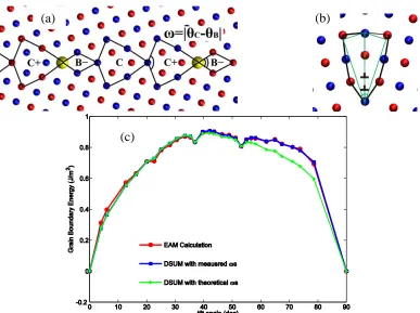
510 structure instead of 36.87° predicted by CSL theory. We measured disclination angle differences for all those grain boundary structures that have 𝐶 − 𝐷 dislination dioples and took the average value as the input parameter, i.e. 𝜔_𝐶𝐷, in Eqs (2-1) and (3-9). Following this procedure we measured the diople strengths of different structural units for all four alloy systems and list the values in Table 2.2. From Table 2.2, we can see that the actual 𝜔_𝐴𝐵 and 𝜔_𝐵𝐶 values are approximatly equal to the ideal values, while 𝜔_𝐶𝐷 values are clearly greater. We believe that the degree to which the grain boundary structure resembles the dislocation wall model plays an essential role here. As illustrated in Figure 2.1- (b), the actual basic unit C structure differs widely from the uniformly distributed dislocation wall model. which is the assumed in Eqs (2-1) and (3-9). Instead, constrained by geometries, the two dislocations inside C are pushed aside by the middle atom and piled up at at the bottom of the unit. This pile up gives the 𝐶 − 𝐷 diople a larger value of 𝜔. This modification to diople strengths have a pronounced effect on DSUM predictions. As shown in Figure 2.1-(c), using unrealistic 𝜔 values for 𝐶 − 𝐷 dioples underestimates the grain boundary energy of copper in the high tilt angle region. The difference is the energy needed to pile up the two dislocaions.

Figure 2.2 summarizes the misorientation angle dependences of grain boundaries energies of both pure metal systems and alloy systems determined from atomistic

would expect to see from EAM calculations at almost all tilt angles. Similar results have been obtained for many pure metal systems over the past decades [25], [27], [28].

Stabilization effects are clearly demonstrated in Figure 2.2, in which the doped structures give lower grain boundary energies than that of dilute solutions in pure metal structures. The grain boundary energy of the doped system at tilt angle of 0o _{and 90}o _are

hypothetical since these two structures are grain- boundary-free lattices. In our calculation we hypothetically chose (110) and (100) as grain boundary planes. To compare results of hypothetical grain boundaries to normal ones, we artificially choose those doped sites that lie on (110) and (100) planes whereas doped sites in defect-free0lattice should be distributed homogenously among the lattice in the dilute solution limit.

A notable result from Figure 2.2 is that grain boundary energies of some doped structures are negative for some structures, for example the Σ13 − 320 and Σ17 − 410 interfaces in Cu-Zr and Al-Pb systems. In the case of dilute solute systems, a negative grain energy means that the grain boundary structure is more stable than the perfect lattice

structure. If an alloy of such material is recovered from work hardening, grains enclosed by negative energy grain boundaries are not driven to grow because the energy change of removing those grain boundaries is positive.

lattice constant difference 𝛿𝑎_𝐼𝑀 = |𝑎_𝐼− 𝑎_𝑀|, where 𝑎_𝐼 (𝑎_𝑀) is the lattice constant of the solute (matrix) material, we can draw the phenomenological conclusion from Figure 2.3 that the stabilization energy is negatively correlated to 𝛿𝑎𝐼𝑀. For example, zrconium has a more

prominent stabilizing effect to copper than niobium. This is because 𝑎_{𝑍𝑟−𝐶𝑢} ≈ 0.38Å >

𝛿𝑎_{𝐶𝑢−𝑁𝑏} ≈ 0.31 Å . This empirical conclusion is reasonable, because the volume misfit

effect grows as the lattice constant difference increases.

Figure 2.3-(c) and (d) demonstrates how grain boundary energy changes with area density of impurities. The lines in (c) are not smooth, and taking Cu – Nb system as an example, there are five linear segments in the blue line. Each stage corresponds to a doping level. As concentration of Nb in Cu is gradually increased, impurities tend to sit on those sites with lowest substitutional energies. In the meantime, it is apparent from Figure 2.3-(b) that there are many sites with similar energies in a grain boundary model. We therefore call this stage 1st doping level region in which substitution happens only at energy favorites sites.

smaller optimized grain boundary energy is not straightforward. Considering that the unit A does not bring any defect into the structure, but B does. As the tile angle increases, the proportion of B units also increases, and thus more defects are introduced, and the interaction between defects and grain boundary are then increased accordingly because the total stress field is also increasing.

2.5 Conclusion

In this chapter, several efficient computational methods were presented to study the stability of alloy systems. First, a formula based on the perturbation of EAM potentials was derived and implemented in LAMMPS to compute the in-place substitution energy for all lattice sites for all atom models. This algorithm is 𝑂(𝑁2_{) in time compared to 𝑂(𝑀 × 𝑁}2_{) of}

conventional methods if 𝑁 lattice sites are present and 𝑀 substitution sites are considered. Second, for grain boundaries with solute segregated at favorite segregation sites or the second to most likely segregate lattice sites, a formula based on DSUM techniques was proposed to compute the corresponding grain boundary energies. Because the DSUM is a macroscopic model and has analytical expression for grain boundary energies, its complexity in time can be considered as 𝑂(1). In contrast, computing corresponding grain boundary energies with molecular dynamics requires at least 𝑂(𝑁 log 𝑁) computation time, not to mention the formidable tasks of building full atomistic models for every grain boundary investigated. Third, we constructed a three-fold method to compute substitution energy for every lattice site with expansion techniques. Compared to the conventional way of

of molecular dynamics steps for potential energy minimization, this method is 𝑂(𝑁2_{) n time}

and therefore can save enormous computation effort since it allows us to compute the segregation energy at arbitrary lattice sites without performing structural relaxation or doing solute substitution one at a time. All three proposed methods have been tested with

satisfactory accuracy for for various alloy systems.

Figure 2.1: (a) Structural units model of FCC 〈100〉-Σ73-830 grain boundary. Impurity atoms, which are represented by bigger yellow spheres, segregate on the first lowest energy sites. The blue and red spheres denote the copper atoms that lie on (002) and (001) planes respectively. Those structures whose head (tail) atom is replaced are marked as positive (negative) structure. (b) Illustration of theoretical (inside green shape) and actual (outside black shape) C structure. Two dislocations pile up at the bottom of C unit. (c) Illustration how disclination dipole strength affects the DSUM results, the red dot line is the grain boundary energy of Copper calculated from atomistic models. The blue rectangle line and the green triangle line are DSUM predictions with and without dipole strength modification respectively.

(a)

(c)

(a) _(b)

(c) (d)

Figure 2.2: Dependence of energies of 〈100〉 symmetric tilt grain boundaries on the tilt angle for four systems.

(a)

(b)

(c) (d)