Article
Efficiency Evaluation of Wastewater Pollution and Water
Disease Efficiency in China Based on the Dynamic
Two-Stage DEA Method
Sun yanan1, Ren Fangrong2*, Liu jiawei1 and Shi Naixin1
1 Economics and Management School, Nantong University, No.9 Seyuan Road, Nantong, Jiangsu 226019, China,
P.R; Email: [email protected]; [email protected]; [email protected]
2 Business School, Hohai University, Nanjing 211100, China, P.R; [email protected]
* Correspondence: [email protected]
Abstract: China is not only short of fresh water resources per capita, but also faces a serious problem of
water pollution in recent years, with 190 million people suffering from excessive levels of harmful substances in their drinking water. Such as arsenic poisoning and fluorosis and other endemic water diseases high incidence. As a series of water pollution prevention plan of action by the Chinese government announced that, this paper uses the modified Undesirable Dynamic Network model empirical analysis of China's 31 provincial administrative region economic growth, wastewater treatment, and water disease control efficiency between 2013 and 2017. The results show that the efficiency of water pollution disease in all four regions of China and the total efficiency in the three regions of east, west and central China all show a decreasing trend, and the efficiency scores and rankings of all provinces and cities within the region fluctuate greatly. The eastern region with the most developed economy has the best overall performance, with higher efficiency in Water consumption and Water disease control. However, the efficiency of wastewater treatment in northeast China is stable and better. Given the high level of economic development in China and the results of the above mentioned efficiency in water pollution and water diseases, improving the efficiency and quality of wastewater treatment in China is regarded as an important factor in achieving the strategic goal of green growth.
Keywords: Dynamic network DEA; efficiency; wastewater Pollution; Water diseases
1. Introduction
Water is the basic requirement for maintaining life and health, and although 70.8% of the earth is covered by water, fresh water resources are still extremely limited. In the face of increasing demand, water issues are a top priority to resolve for any country targeting economic growth. At present, China’s social and economic development ranks at the forefront of the world, but its water shortage problem is very serious. At the end of 2018, the country had total water resources of 2,796 billion cubic meters or 2,004 cubic meters per person, taking up one quarter of the world’s average. China is one of 13 water-poor countries in the United Nations, especially in the north and parts of the east where per capita water resources are seriously low. However, with the continuous development of its economy and the increasing living standard of residents, water consumption continues to be very high, with the total water consumption of 611 billion cubic meters in 2018.
Another situation that is more mismatched than water shortages is the serious problem of water pollution in China. In 2017, China’s total wastewater discharge was 69.97 billion tons: industrial wastewater discharge at 18.16 billion tons, or 26.0% of total emissions, and urban domestic sewage discharge at 51.78 billion tons, or 74.0% of total discharge. The proportion of urban domestic sewage is increasing year by year and is the main source of sewage. In 2017, the “Bulletin on the Circumferential
Situation of Ecology in China” reported 940 surface water quality sections that the proportion of inferior V water quality is 8.3% (V-type water: The quality of V-type water is suitable for agricultural water area and general landscape water area. Inferior type water: The quality of inferior type water is worse than V-type water quality.), and among the 5100 groundwater quality monitoring points the proportion of poorer and lower points is 66.6%. Two-thirds of China’s cities are already facing water shortages, and the already limited clear water resources are being destroyed by discharged sewage, further exacerbating water scarcity.
As water pollution worsens, human health also faces a serious threat. More than 300 million people in China still have unsafe drinking water, of which about 63 million people drink high-fluorine water, 2 million people drink high-arsenic water, 38 million people drink brackish water, and 190 million people drink water with excessive harmful substances. Drinking water contaminated with harmful chemicals can cause corresponding infectious diseases or acute and chronic poisoning. Drinking arsenic, chromium, nickel, strontium, and polycyclic aromated hydrocarbons or halogenated hydrocarbons for a long time can cause damage to the skin and nervous system, generate cardiovascular and cerebrovascular diseases, and cause carcinogenic effects.
The China government has attached great importance to the predicament of water pollution. In 2011, 2015, and 2017, it respectively formulated the National Groundwater Pollution Prevention and Control Plan (2011-2020), the Water Pollution Prevention Action Plan, and the Key Basin Water Pollution Prevention and Control Plan (2016-2020). It has also put forward the development concept of prioritizing saving water, strengthening water resources management, and controlling water pollution to the greatest extent. Therefore, this research contributes to water pollution control and water disease prevention in China.
The present literature on water pollution, wastewater treatment, and water diseases mainly presents the following types: 1) Economic and feasibility study on wastewater treatment; [3-8] 2) Research on wastewater treatment and health; [9-15] and 3) Research on wastewater using DEA (Data Envelopment Analysis). [16-24] However, there is little discussion from the perspectives of the economy, water pollution, and health. Although some studies use regression or DEA methods for efficiency assessment, most of them are based on static analysis, cannot understand the sustainable development of an economy and environment, and fail to consider regional differences and health factors. Therefore, in order to solve the shortcomings of static analysis, regional differences, and health factors, our research proposes a modified undesirable dynamic Network model to explore economic, wastewater treatment, and human health efficiencies of 31 provincial-level administrative regions in China.
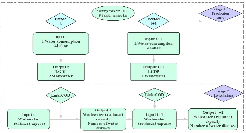
The main contributions of this paper are twofold. First, we study economic, wastewater discharge, and wastewater pollution efficiencies, explore the government wastewater treatment input and water disease efficiency, and comprehensively investigate and sort out the inherent relationship between the economy, environmental pollution, and health. Second, the modified undesirable dynamic network model can avoid the shortcomings and problems of static analysis. In this study the production stage is Stage1 and the health stage is Stage 2. The inputs of Stage 1 are production stage labor and water consumption, the outputs of Stage 1 are GDP and wastewater. The variable that links the production stage and health stage is Chemical Oxygen Demand (COD). The input of Stage 2 is Wastewater treatment expense, the outputs of Stage 2 are Wastewater treatment capacity and Number of water diseases, and the carry-over variable is Fixed Assets. The remainder of this paper is organized as follows: II. Literature Review; III. Research Method; IV. Empirical Results and Discussion; and V. Conclusion.
2. Literature Review
As early as 1999, Wu et al. [1] pointed out that the process of urbanization and industrialization in China had brought about tremendous pollution, coupled with inadequate investment in basic water supply and treatment infrastructure, resulting in extensive wastewater pollution. The extreme waste of water
resources poses a challenge to sustainable development, depleting energy reserves and destroying humans’
Economic and feasibility studies on wastewater treatment; 2) Research on wastewater treatment and health; and 3) Research on wastewater using DEA (data envelopment analysis).
Among economic and feasibility studies of wastewater treatment and wastewater treatment plants, Lim et al. [2] used LCA and LCC research methods to evaluate the environmental and economic feasibility of a complete wastewater treatment network system, including distributed and terminal wastewater treatment plants. Molinos-Senante et al. [3] quantified the environmental benefits of wastewater treatment using the concept of shadow prices to estimate environmental benefits and developed a corresponding cost-benefit analysis (CBA) for each wastewater treatment plant. Hernández-Sancho et al. [4] pioneered the estimation of shadow prices based on the removal of contaminants during processing and expressed the environmental benefits associated with undischarged pollution, comparing the benefits to the internal clearing process. Molinos-Senante et al. [5] combined a cost-benefit analysis tool-based approach with a vast body of knowledge on processing technologies included in the environmental decision support system and applied it to nine scenarios containing different wastewater characteristics and reuse options, obtaining useful economic feasibility indicators such as internal and external costs. Castellet and Molinos-Senante [6] used the non-radial DEA model to incorporate the environmental impacts of each pollutant removed from wastewater treatment plants into the assessment. Sampling efficiency was evaluated and environmental issues were combined with the technical and economic efficiencies of traditional wastewater treatment plants.
The second related research covers wastewater treatment and health. The rapid urbanization and industrialization in the 19th century led to an unhealthy environment and a wide range of epidemics, with research and development of relevant health technologies carried out in response. Akpor and Muchie [7] reviewed the environmental and health effects of untreated or improperly treated wastewater. Estrada et al. [8] found that the social benefits of reducing odor are related to the reduction of nuisances in nearby populations and the improvement of occupational health in sewage treatment plants. Naik and Stenstrom [9] collected samples from 39 different countries, using health, economy, and the environment as research indicators, and concluded that improving the availability of wastewater treatment can reduce disease mortality. He [10] found that surface water pollution has a significant non-linear effect on infant mortality, and water pollution has a significant and negative impact on all elderly people (60 years of age or older) with cancer. Massaquoi et al. [11] collected data to compare the mortality and morbidity of residents living in a wastewater environment and a clean water environment in Shijiazhuang, Hebei province from 2007 to 2011 and suggested limiting or stopping the use of wastewater. Wang and Yang [12] used the random effects model and the random effect logit model to study the relationship between health and water pollution and employed the medium model to evaluate the impact of health through water pollution intensity.
There are also studies on people’s health from gases emitted by the scholars from the wastewater
treatment process. Guan and Chen [13] combined DEA and weighted grey correlation to evaluate the ecosystem of Beijing from 2003 to 2010. The results showed that Beijing has experienced fluctuations in its ecosystem coordination index. The health of employees in wastewater treatment plants has also been studied by scholars. Thorn and Kerekes [14] retrieved articles on wastewater and health in the form of a literature review and how such employees have reported gastrointestinal problems, respiratory symptoms, fatigue, headache, and a higher risk of cancer such as stomach, laryngeal, and pancreas. Masclaux et al. [15] studied the presence and concentration of viruses in the air of wastewater treatment plants and concluded that the potential concentration of viral particles in the air cannot be ignored, which can be used to explain the reasons why employees of this department often report gastrointestinal diseases.
The third is the use of DEA method in wastewater research. Hernández-Sancho [16] employed the non-radial DEA method to calculate the energy efficiency index of a Spanish wastewater treatment plant and the energy efficiency of the wastewater treatment plant was found to be very low. Molinos-Senante [17] utilized DEA to estimate environmental performance indicators (EPI) and incorporated environmental impacts into wastewater treatment plants to assess the efficiency of pure environmental performance indicators (PEPI) and mixed environmental performance indicators (MEPI) for 60 (Spanish wastewater
efficiency of water conservancy institutes and the efficiency of wastewater purification, which were then used to analyze the efficiency of urban water and wastewater purification systems in China.
Huang [19] used the non-radial network DEA method to measure the performance of environmental protection systems in 20 cities in Taiwan. The system consists of three stages: administration, execution, and protection effectiveness. In addition to evaluating efficiency, the impacts of internal and external factors on performance were further discussed. Guerrini [20] used two-stage DEA to analyze Denmark’s water
sector and investigated the scale, scope, and density economy of the wastewater sector. The results showed that its water sector is characterized by economies of scope and density. Zhang et al. [21] employed the dynamic network SBM model to evaluate the production and health efficiency of Chinese cities. The results showed that the productivity score of Chinese cities is slightly higher than that of health efficiency, and that the two-stage efficiency score of most cities fluctuates significantly.
Hu et al. [22] combined bi-level planning (BLP) and DEA with feedback variables to demonstrate the applicability and effectiveness of case studies in 10 cities along the Lancang River Basin. Each DMU was sorted using super-efficient DEA, and the results showed that the proposed model is more discriminative. Lorenzo-Toja et al. [23] studied 113 wastewater treatment plants in Spain using a combination of life cycle assessment (LCA) and data envelopment analysis (DEA). At the same time, in order to verify the eco-efficiency criteria, the environmental benefits associated with the reduced input suggested by the DEA
model for each unit were calculated. D’Inverno et al. [24] studied the environmental efficiencies of 96 Tuscan (Italy) wastewater treatment plants using a new integrated Analytic Hierarchy Process/Non-radial Directional Distance Function (AHP/NDDF), in which the treated water, which was treated with residual nitrogen, was an undesirable output. The random output means that the capacity of the facility, the percentage of wastewater discharged from industrial and agricultural activities, and the threshold for pollutant concentration have a large impact on processing efficiency.
At present, the commonly used comprehensive index evaluation methods mainly include analytic hierarchy process (AHP), principal component analysis (PCA), Fuzzy comprehensive evaluation method (FCE), Topsis and so on. DEA is a kind of evaluation method which can consider many input-output indexes at the same time. Its advantage is that it can compare multiple decision making units, and can select the input-output index flexibly according to the characteristics of the evaluation object, so as to establish the evaluation index system more in line with the analysis needs. The dynamic two-stage DEA method used in this paper, combined with the logical progression of time series and two-stage events, can better see the correlation between water pollution and water disease as well as the change of efficiency. Most current studies have not been discussed together from the economic, water pollution, and health aspects, and the DEA methods are mostly static and do not combine wastewater discharge and COD as unexpected output with a dynamic DEA model. Our study makes up for the shortcomings in this area, in order to call for and bring attention to water pollution and water diseases and put forward corresponding effective suggestions and measures.
3. Method and Model
3.1. SBM dynamic network DEA
time, because a company’s operation spans many periods, we use the Dynamic DEA model, and if we need to evaluate departments and time at the same time, then we can combine Network DEA and Dynamic DEA. Tone and Tsutsui (2013) put forward the weighted SBM (weighted slack-based measures) Dynamic Network DEA data envelopment analysis model, based on the analysis of the network DEA model of linkages between different departments of decision-making units and regarded each department as a sub-DMU and carry-over activities as linkages (l). As a form of linkage, the carry-over activities can be divided into four categories: (1) desirable, (2) undesirable, (3) discretionary, and (4) non-discretionary.
3.2. The modified undesirable dynamic network model
This study utilizes panel data collected from 31 provincial administrative regions in China. Labor input and water consumption are set as input indicators, while GDP and Wastewater are the output indicators to analyze wastewater efficiency and economic efficiency in the first stage of each province. Water pollutant COD is a link indicator, wastewater treatment expense is an input indicator, and wastewater treatment capacity and number of water diseases are output indicators in the second stage. Carry-over variable assets are fixed assets to help evaluate the efficiency of government wastewater input in each province. Since this study considers undesirable output in the dynamic network SBM model, we modify Tone and Tsutsui’s
(2013) dynamic network model to be the undesirabledynamic network model and set it up as follows.
Modified undesirable dynamic network model
Suppose there are n DMUs (j = 1,…,n), with each having k divisions (k = 1,…,K) and T time periods (t =
1,…,T). Each DMU has an input and output at time period t and a carryover (link) to the next t+1 time period. We set
m
k andr
k as the input and output in each divisionK
, with( )i
k,h representing divisionsk
toh
, andL
hk is thek
andh
division set. The input and output, links, andcarryover definitions are outlined in the following.
Inputs and outputs
+
R
X
ijkt(
i
=
1
,...,
m
k;
j
=
1
,...,
n
;
K
=
1
...,
K
;
t
=
1
,...,
T
)
: refers to inputi
at time periodt
for jDMU
divisionk
.+
R
y
rjkt(
r
=
1
,...,
r
k;
j
=
1
,...,
n
;
K
=
1
...,
K
;
t
=
1
,...,
T
)
: refers to output r in time period t forDMU
jdivision
k
; if part of the output is not ideal, then it is considered an input for the division.Links
+
R
Z
tj(kh)t(
j
=
1
;...;
n
;
l
=
1
;..;
L
hk;
t
=
1
;...;
T
)
0
: refers to the period t links fromDMU
j divisionk
to divisionh
, withL
hk being the number ofk
toh
links, and Ztj(kh)t ∈R+(j =1,…,n; l = 1,…,Lkh; t = 1,…,T).Carryovers
+
+
R
Z
jkl(t,t 1)(
j
=
1
,...,
n
;
l
=
1
,..,
L
k;
k
=
1
,...
k
,
t
=
1
,...,
T
−
1
)
: refers to the carryover oft
to thet
+
1
period from
DMU
j divisionk
to divisionh
, withL
k being the number of carryover items indivision
k
.The following is the non-oriented model.
Overall efficiency:
= = = = − + = = = + + = −
+
+
+
+
+
+
+
−
=
T t K k r r r t rokbad t rokbad t rokgood t rokgood k k k t T t K k linkin kh ninput k t t input ok t t input ok t in kh o t in kh o m i t iok t iok k k k k t k k k l k l l l l l ky
s
y
s
r
r
W
W
z
s
z
s
x
S
ninput
linkin
m
W
W
1 1 1 r1
2 1
1 1 ( ) 1 (, 1)
) 1 , ( ) ( ) ( 1 * 0
)
(
1
1
)
(
1
1
min
1 2
Subject to: −
+
=
t ko t k t k tok
X
s
x
)
,
(
k
t
+
−
=
t kogood t k t kgood tokgood
Y
s
y
)
,
(
k
t
−
+
=
t kobad t k t kbad tokbad
Y
s
y
)
,
(
k
t
1
=
t ke
)
,
(
k
t
,
0
t k
s
kot−
0
,
t+
0
,
kogood
s
0
,
− t kobad
s
)
,
(
k
t
t in kh o t k t in kh t in kh
o
Z
S
Z
( )=
( )
+
( ))
,...,
1
)
((
kh
in
=
linkin
k1 1 )) 1 ( , ( 1 )) 1 ( , ( 1 1 + = + = +
=
tjk n j t t jk t jk n j t t jk
z
z
)
1
,...,
1
;
;
(
k
k
lt
=
T
−
)) 1 ( , ( )) 1 ( , ( 1 )) 1 ( , ( + + =
+
=
+
t tinput ok t jk t t input jk n j t t input ok l l
l
z
s
Z
k
l=
1
,...,
ngood
k;
k
;
t
)
,
0
)) 1 ( , (t t+
good okl
s
(
k
l;
t
)
(b) Period and division efficiencies
Period and division efficiencies are as follows:
(b1) Period efficiency:
= = + + = − + = = = −
+
+
+
+
+
+
+
−
=
K k r r ngood k t t good ok t t good ok r t rokbad t rokbad t rokgood t rokgood k k k k K k linkin kh t in kh o t in kh o m i t iok t iok k k k k k l l l k k l l l kz
s
y
s
y
s
ngood
r
r
W
z
s
x
S
linkin
m
W
1 1 (, 1)
) 1 , ( 1 r 2 1
1 ( ) 1
) ( ) ( 1 * 0
)
(
1
1
)
(
1
1
min
1 2
= = = − + = = + + = −
+
+
+
+
+
+
+
−
=
T t r r r t rokbad t rokbad t rokgood t rokgood k k t T t linkin kh ninput k t t input ok t t input ok t in kh o t in kh o m i t iok t iok k k k t k k k l k l l l l l ky
s
y
s
r
r
W
z
s
z
s
x
S
ninput
linkin
m
W
1 1 r 1
2 1
1 ( ) 1 (, 1)
) 1 , ( ) ( ) ( 1 * 0
)
(
1
1
)
(
1
1
min
1 2
(b3) Division period efficiency:
)
(
1
1
)
(
1
1
min
1 21 r 1
2 1
1 )
( (, 1)
) 1 , ( ) ( ) ( 1 * 0
= = − + = + + = −+
+
+
+
+
+
+
−
=
k k k l k l l linput l l k r r r t rokbad t rokbad t rokgood t rokgood k k linkin kh ninputk okttinput t t input ok t in kh o t in kh o m i t iok t iok k k k
y
s
y
s
r
r
z
s
z
s
x
S
ninput
linkin
m
3.3.
Labor, Water consumption, Wastewater treatment expense, GDP, Wastewater treatment capacity, Wastewater, COD and Water diseasesThere are eight key features of this present study: Labor efficiency, Water consumption efficiency, Wastewater treatment expense efficiency, GDP efficiency, Wastewater treatment capacity efficiency, Wastewater efficiency, COD efficiency, and Water diseases. In our study, “I” represents area and “t”
represents time. The eight efficiency models are defined in the following. Labor efficiency = Actual labor input (i,t)Target labor input (i,t)
Water consumption efficiency = Target water input (i,t)
Actual water input (i,t)
Wastewater treatment expense efficiency = Target expense input (i,t)Actual expense input (i,t)
GDP efficiency = Actual GDP desirable output (i,t)Target GDP desirable output (i,t)
Wastewater treatment capacity efficiency = Actual capacity desirable output (i,t)Target capacitydesirable output (i,t)
Wastewater efficiency = Target Wastewater Undesirable output (i,t)Actual Wastewater Undesirable output (i,t)
COD efficiency = Target COD Undesirable output (i,t)
Actual COD Undesirable output (i,t)
Water diseases = Target diseases Undesirable output (i,t)Actual diseases Undesirable output (i,t)
If the target labor, Water consumption, and Wastewater treatment expense inputs equal the actual inputs, then the labor, Water consumption and Wastewater treatment expense efficiencies equal 1, indicating overall efficiency. If the target inputs are less than the actual inputs, then the labor, Water consumption and Wastewater treatment expense efficiencies are less than 1, indicating overall inefficiency.
If the target Wastewater, COD, and Water diseases undesirable outputs equal the actual undesirable outputs, then Wastewater, COD, and Water diseases efficiencies equal 1, indicating overall efficiency. If the target undesirable outputs are less than the actual undesirable outputs, then the Wastewater, COD, and Water diseases efficiencies are less than 1, indicating overall inefficiency.
desirable outputs, then the GDP and Wastewater treatment capacity efficiencies are less than 1, indicating overall inefficiency.
4. Empirical Study
4.1. Data sources and description
This paper collects data of 31 provincial administrative regions in China from 2013 to 2017. The division of the eastern, central, western, and northeastern regions refers to the regional division standards published on the website of the National Bureau of Statistics of China. The eastern region includes Beijing, Tianjin, Hebei, Shanghai, Jiangsu, Zhejiang, Fujian, Shandong, Guangdong, and Hainan (10 provinces (cities)); the central region includes Shanxi, Anhui, Jiangxi, Henan, Hubei, and Hunan (6 provinces); the western region includes Inner Mongolia, Guangxi, Chongqing, Sichuan, Guizhou, Yunnan, Shaanxi, Gansu, Qinghai, Ningxia, Xinjiang, and Tibet (12 provinces (municipalities and autonomous regions)); and the northeast region includes Liaoning, Jilin, and Heilongjiang (3 provinces). The data were extracted from the Statistical Yearbook of China, the Demographics and Employment Statistical Yearbook of China, the Environmental Yearbook of China, and the Health Statistics Yearbook of China. Figure 1 reveals the framework of the Dynamic Network Model of inter-temporal efficiency measurement and variables.
Figure 1. Dynamic Network Model.
Table 1 shows all the input and output variables of the two stages. There are three inputs, four outputs, one link and one carry-over variables.
Table 1. Input and output variables.
Input variable Output variable Link Carry-over
Stage 1 Labor GDP
COD Fixed assets Water consumption Wastewater
Stage 2 Wastewater treatment expense
Number of water diseases
Stage 1: Production Stage Input variables:
Labor: This study takes the numbers of employees in each region by the end of each year. Unit: 10,000
persons.
Water consumption: Gross amount of water taken by various water users, including loss of water delivery.
Unit: 100 million tons.
Fixed assets: The total amount of work done by the whole society in building and purchasing fixed assets
and related expenses. Unit: 100 million RMB.
Output variables:
Desirable output (GDP): Refers to the final result of production activities of all resident units in a region
calculated by market price in a year. Unit: 100 million RMB.
Undesirable output (Wastewater): It is the sum of industrial wastewater discharge and domestic sewage
discharge. Unit: 10,000 tons.
Link Production Stage and health stage variables:
COD: The sum of chemical oxygen demand (COD) emissions from industrial wastewater and domestic wastewater. It refers to the amount of oxygen required to oxidize organic pollutants in water analyzed by chemical oxidizers.
Stage 2: Health Stage Input variable:
Wastewater treatment expense: The annual investment amount of each district’s wastewater treatment
project. Unit: 10,000 RMB.
Output variables:
Desirable output (Wastewater treatment capacity): The amount of wastewater actually treated by various
water treatment facilities. Unit: 10,000 tons.
Undesirable output (Number of water diseases): The number of water diseases caused by drinking
polluted water and mainly includes fluorosis and arsenic poisoning. Water fluorosis and arsenic poisoning are two typical water poisoning diseases in China1. Unlike water diseases caused by common bacterial infections, they are chronic and regionally widespread. Unit: persons.
4.2. Statistical analysis of input-output indicators
1. From document No. 2004375 of the State Council of China, national key endemic disease prevention and control program (2004-2010).
0.00 500.00 1,000.00 1,500.00 2,000.00 2,500.00
Average Max Min St.Dev
2013Labor 2014Labor 2015Labor
2016Labor 2017Labor
0 500 1000
Average Max Min St.Dev
Figure 2. Statistical Analysis of Labor, Water Consumption, Wastewater Production, Wastewater Treatment Expense, COD, and Number of Water Diseases, 2013-2017.
Figure 2 shows the changes of input-output indicators. From 2013 to 2017, the maximum and minimum values of labor input increased slowly, and the average value decreased slightly. This is mainly due to the disappearance of China’s demographic dividend and the slowdown of its population growth. At the same time, the number of working-age population gradually declined.
The average and maximum values of wastewater discharge fluctuated distinctly. After peaking in 2015, the average declined again in 2016-2017. The maximum value continued to rise over 2013-2016, and after peaking in 2016, there was a significant decline in 2017. The standard deviation also showed a trend of rising first and then falling, which indicates that regional differences are narrowing.
The maximum input of wastewater treatment expense has decreased significantly since 2014. The trend of average decline was also obvious. It showed that the investment cost of wastewater treatment in various provinces and municipalities in China was decreasing year by year.
As the most important indicator of water pollution, COD has declined significantly after 2015, which means that the China government’s promulgation and implementation of the new "Environmental Protection Law" and "Water Pollution Prevention and Control Action Plan" in 2015 had remarkable results. However, it is noteworthy that the maximum COD in 2017 rebounded to upward trend compared with 2016, which means that water pollution in individual provinces and cities was aggravated again.
The average number of water pollution diseases showed a slow downward trend, but the maximum value decreased significantly between 2016 and 2017, denoting that there are obvious regional differences in water pollution diseases. The areas with high incidences of water pollution diseases need more careful control, and the situation of prevention and control of water pollution diseases in China is still serious.
0.00 200,000.00 400,000.00 600,000.00 800,000.00 1,000,000.00
Average Max Min St.Dev
2013Wastewater 2014Wastewater
2015Wastewater 2016Wastewater
2017Wastewater
0.00 20,000.00 40,000.00 60,000.00 80,000.00 100,000.00 120,000.00 140,000.00 160,000.00 180,000.00 200,000.00
Average Max Min St.Dev
2013treatment expense 2014treatment expense
2015treatment expense 2016treatment expense
2017treatment expense
0 20 40 60 80 100 120 140 160 180 200
Average Max Min St.Dev
2013COD 2014COD 2015COD
2016COD 2017COD
0.00 1,000,000.00 2,000,000.00 3,000,000.00 4,000,000.00 5,000,000.00 6,000,000.00
Average Max St.Dev
2013Number of water diseases
2014Number of water diseases
2015Number of water diseases
2016Number of water diseases
4.3. Analysis of the total efficiency of the provinces from 2013 to 2017
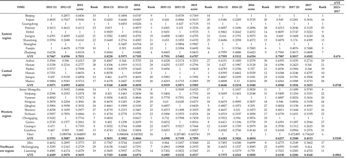
Figure 3 shows that the total efficiency scores of provinces, municipalities, and autonomous regions fluctuate greatly from 2013 to 2017. The provinces, municipalities, and autonomous regions with a total efficiency score of 1 in 2017 include Beijing, Guangdong, Shanghai, and Chongqing. Chongqing is in the western region, while the others are in the eastern region. Some provinces, municipalities, and autonomous regions presented a steep increase in 2016, whose total efficiency score increased significantly, such as compared with the previous year, Beijing increased by 35.7% and Guangdong by 40.15%. In 2014, the average score of total efficiency in Northeast China rose from 0.3603 in 2013 to 0.6576. In 2015, Some provinces increased significantly. For example, compared with 2014, Gansu increased by 201.47% and Qinghai by 164.55%. However, these provinces generally fell sharply in the year after their sharp rise, which led to a downward trend in the eastern, central, and western regions, except for the average level of total efficiency in the northeast region. Although the average score of total efficiency in the eastern region decreased from 0.7031 to 0.6502, it remains the best among the four regions.
Figure 3. Total Efficiency Scores of Provinces, Municipalities, and Autonomous Regions from 2013 to 2017.
From the total efficiency ranking, the ranking of most cities fluctuates greatly, and the provinces with higher ranking are Beijing, Shanghai, Jiangsu, Shandong, and Tianjin in the eastern region. With great fluctuation, the northeastern region has all been on the rise. From this we can see that the rankings of most provinces and cities in the central and eastern regions declined, while the rankings of provinces and cities in the northeast and western regions increased significantly.
Table 2 shows that the provinces, municipalities, and autonomous regions with a total efficiency of 1 for five consecutive years are Beijing, Guangdong, Inner Mongolia, Shanghai, Tianjin, and Tibet. In the eastern, western, and northeastern regions, the average level of total efficiency scores in the first stage has been rising. In Stage1, the total efficiency scores of most cities in China also showed an upward trend, with Chongqing and Qinghai showing the greatest increase. The average level of the total efficiency score in Stage1 of the eastern region was relatively stable and the best among the four regions. The average water fluctuation of the first stage efficiency score in the central region was not significant, but overall declined. The average levels of Stage1 in the western and northeastern regions made remarkable progress.
The total efficiency score of Stage2 was quite different from that of Stage1. For example, in 2017 the efficiency score of Tianjin in Stage1 was 1, and that in Stage 2 was only 0.4976. In 2013, their total efficiency scores in Stage2 were all DEA effective, and in 2017 these provinces all dropped to below 0.5.
0 0.2 0.4 0.6 0.8 1 1.2
A
n
h
u
i
Bei
jin
g
Fu
jian
G
an
su
G
u
an
gd
o
n
g
Gu
an
gx
i
G
u
iz
h
o
u
H
ain
an
H
eb
e
i
H
en
an
H
ei
lo
n
gjian
g
H
u
b
ei
Hu
n
an Jilin
Jian
gs
u
Jian
gx
i
liao
n
in
g
In
n
er Mo
n
go
lia
N
in
gx
ia
Q
in
gh
ai
Sh
an
gd
o
n
g
Sh
an
xi
Sh
aan
xi
Sh
an
gh
ai
Si
ch
u
an
Ti
an
jin
Ti
b
e
t
Xin
jian
g
Yu
n
n
an
Zh
ejian
g
Ch
o
n
gq
in
g
Table 2Total Efficiency Scores and ranks of Provinces, Municipalities, and Autonomous Regions from 2013 to 2017.
DMU 2013 (1) 2013 (2) 2013
score Rank 2014 (1) 2014 (2) 2014
score Rank 2015 (1) 2015 (2) 2015
score Rank 2016 (1) 2016 (2) 2016
score Rank 2017 (1) 2017 (2) 2017 score Rank
AVE 2013-2017
Eastern region
Beijing 1 0.2871 0.6436 15 1 0.3494 0.6747 9 1 0.4739 0.7369 14 1 1 1 1 1 1 1 1
Fujian 0.4835 0.7017 0.5926 16 0.6203 0.6646 0.6425 13 0.626 0.4966 0.5613 20 0.5186 0.2285 0.3735 20 0.545 0.2381 0.3916 16
Guangdong 1 1 1 1 1 0.6453 0.8226 6 1 0.427 0.7135 15 1 1 1 1 1 1 1 1
Hainan 0.3612 0.4612 0.4112 23 0.815 1 0.9075 3 0.4201 0.231 0.3256 26 0.4097 0.1696 0.2896 28 0.4213 0.2046 0.3129 25
Hebei 1 1 1 1 0.9029 1 0.9514 1 0.9451 1 0.9725 3 0.5861 0.2642 0.4252 14 0.8697 0.1747 0.5222 9
Jiangsu 0.4391 0.4095 0.4243 21 0.5582 0.4002 0.4792 19 0.6008 0.3401 0.4705 23 0.616 0.1791 0.3975 16 0.669 0.1608 0.4149 14
Shandong 0.5594 0.2688 0.4141 22 0.6449 0.2716 0.4583 21 0.653 0.1855 0.4192 25 0.6686 0.2058 0.4372 13 0.6878 0.174 0.4309 13
Shanghai 1 1 1 1 1 0.3407 0.6704 10 1 0.9894 0.9947 2 1 1 1 1 1 1 1 1
Tianjin 1 0.4678 0.7339 10 1 0.301 0.6505 12 1 0.3384 0.6692 16 1 0.5766 0.7883 6 1 0.4976 0.7488 5
Zhejiang 0.6236 1 0.8118 5 0.6964 1 0.8482 4 0.6865 1 0.8433 4 0.7959 0.4886 0.6423 9 0.7943 0.5673 0.6808 7
AVE 0.7467 0.6596 0.7031 0.8238 0.5973 0.7105 0.7931 0.5482 0.6707 0.7595 0.5112 0.6354 0.7987 0.5017 0.6502 0.674
Central region
Anhui 0.3566 0.506 0.4313 20 0.4067 0.344 0.3753 24 0.4328 0.2174 0.3251 27 0.4151 0.1005 0.2578 30 0.4393 0.1035 0.2714 29
Henan 0.3338 0.2216 0.2777 28 0.4306 0.1919 0.3112 28 0.4255 0.1337 0.2796 31 0.427 0.1987 0.3128 24 0.4396 0.2423 0.341 21
Hubei 0.5717 1 0.7858 6 0.5308 0.5579 0.5443 15 0.6856 1 0.8428 6 0.4783 0.2356 0.357 21 0.4936 0.1984 0.346 19
Hunan 0.7351 1 0.8676 4 0.8538 1 0.9269 2 1 1 1 1 0.6595 0.4462 0.5529 12 0.6348 0.3246 0.4797 10
Jiangxi 0.457 0.9139 0.6854 12 0.461 0.4775 0.4693 20 0.5983 1 0.7992 9 0.4067 0.2295 0.3181 23 0.5228 0.1781 0.3504 18
Shanxi 0.5884 0.5541 0.5712 17 0.4178 0.2427 0.3302 26 0.4215 0.1715 0.2965 29 0.4008 0.13 0.2654 29 0.4341 0.1088 0.2715 28
AVE 0.5071 0.6993 0.6032 0.5168 0.4690 0.4929 0.5939 0.5871 0.5905 0.4646 0.2234 0.3440 0.4940 0.1926 0.3433 0.4748
Western region
Inner Mongolia 1 0.3692 0.6846 14 1 0.4396 0.7198 8 1 0.3049 0.6525 17 1 0.1657 0.5828 11 1 0.1498 0.5749 8
Xinjiang 0.2596 0.2553 0.2574 30 0.421 0.1463 0.2836 30 0.5404 1 0.7702 10 0.3695 0.1401 0.2548 31 0.5409 0.1254 0.3331 22
Yunnan 0.4943 1 0.7472 8 0.5056 0.4632 0.4844 18 0.7778 0.7551 0.7664 11 1 1 1 1 0.4807 0.2024 0.3416 20
Ningxia 0.3878 0.2204 0.3041 26 0.4678 0.1283 0.298 29 0.63 0.6245 0.6273 18 0.6679 0.0995 0.3837 18 0.546 0.0856 0.3158 24
Qinghai 0.3906 0.3958 0.3932 24 0.4461 0.1909 0.3185 27 0.6857 1 0.8429 5 0.4827 0.1072 0.295 27 0.8024 0.1158 0.4591 12
Shaanxi 0.4258 0.1695 0.2977 27 0.4719 0.2215 0.3467 25 0.4573 0.1498 0.3035 28 0.4637 0.231 0.3473 22 0.4811 0.1444 0.3127 26
Sichuan 0.5857 0.7876 0.6866 11 0.4734 0.2778 0.3756 23 0.5496 0.3553 0.4524 24 0.4519 0.3197 0.3858 17 0.4739 0.1651 0.3195 23
Chongqing 0.5432 1 0.7716 7 0.6834 1 0.8417 5 0.732 0.7598 0.7459 13 0.7812 0.394 0.5876 10 1 1 1 1
Gansu 0.2745 0.1377 0.2061 31 0.402 0.1298 0.2659 31 0.6032 1 0.8016 8 0.6411 0.1106 0.3758 19 0.4391 0.1497 0.2944 27
Guangxi 0.471 1 0.7355 9 0.5032 0.3744 0.4388 22 0.6071 0.9217 0.7644 12 0.4169 0.1789 0.2979 26 0.3938 0.1312 0.2625 30
Guizhou 0.467 0.903 0.685 13 0.4743 0.5264 0.5004 17 0.6053 1 0.8027 7 0.4542 0.3746 0.4144 15 0.4168 0.0984 0.2576 31
Tibet 1 0.089786 0.544893 18 1 0.086604 0.543302 16 1 0.207483 0.603741 19 1 1 1 1 1 0.472495 0.736247 6
AVE 0.5351 0.5887 0.5619 0.5831 0.3902 0.4866 0.6990 0.7199 0.7095 0.6282 0.3426 0.4854 0.6237 0.2388 0.4313 0.5349
Northeast ern region
Jilin 0.4652 0.2895 0.3773 25 0.7567 0.5744 0.6655 11 0.844 0.1657 0.5048 22 0.7493 0.6306 0.6899 8 0.4775 0.2549 0.3662 17
Heilongjiang 0.3295 0.2163 0.2729 29 0.8138 0.6443 0.7291 7 0.4963 0.0908 0.2935 30 0.4633 0.1537 0.3085 25 0.6595 0.1685 0.414 15
Liaoning 0.4981 0.4174 0.4578 19 0.5605 0.5957 0.5781 14 0.7302 0.3832 0.5567 21 1 0.5179 0.759 7 0.7021 0.2385 0.4703 11
1
Figure 4a. Water Consumption Efficiency in Provinces, Municipalities, and Autonomous Regions from 2013
2
to 2017.
3
4
Figure 4b. Labor Efficiency of Provinces, Municipalities, and Autonomous Regions from 2013 to 2017.
5
6
Figure 4c. Wastewater Treatment Cost and Efficiency in Provinces, Municipalities, and Autonomous Regions
7
from 2013 to 2017.
8
Figures 4a-4c reflect the efficiency changes of water consumption, labor force, and wastewater 9 treatment cost. 10 0 0.5 1 1.5 A n h u i Bei jin g Fu jian G an su G u an gd o … G u an gx i G u iz h o u H ain an H eb e i H en an H ei lo n gji… H u b ei H u n
an Jilin
Ji an gs u Jian gx i liao n in g In n er… N in gx ia Q in gh ai Sh an gd o n g Sh an xi Sh aan xi Sh an gh ai Si ch u an Ti an jin Ti b e t Xin jian g Yu n n an Zh ejian g Ch o n gq in g
2013 water consumption 2014 water consumption 2015 water consumption
2016 water consumption 2017 water consumption
0 0.2 0.4 0.6 0.8 1 1.2 A n h u i Be ijing Fuji an G an su G u an gdon g G u an gxi G u izh ou Ha in an He be i He n an He ilon g jia n g Hu bei Hu n
an Jilin
Ji an gs u Ji an gxi lia on in g In n er … Ni n gx ia Qi n gh ai Sh an gd on g Sh an xi Sh aa n xi Sh an gh ai Si ch u an Ti an jin Ti be t Xin jia n g Yu n n an Z h ej ia n g C h on gqing
2013 labor 2014 labor 2015 labor 2016 labor 2017 labor
0 0.2 0.4 0.6 0.8 1 1.2 A n h u i Be ijing Fuji an G an su G u an gd ong G u an gxi G u izh ou Ha in an He be i He n an He ilong jia n g Hu be i Hu n
an Jilin
Ji an gs u Ji an gxi lia on in g In n er M ongo lia N in gxia Qi n gh ai Sh an gd ong Sh an xi Sh aa n xi Sh an gh ai Si ch u an Ti an jin Ti be t Xin jia n g Yu n n an Z h ej ia n g C h on gqing
2013 wastewater treatment expense 2014 wastewater treatment expense
2015 wastewater treatment expense 2016 wastewater treatment expense
Water consumption efficiency has fluctuated with a decrease in Fujian, Guizhou, Hainan, Hebei, 11
Hubei, Hunan, Jiangxi, Ningxia, Shanxi, Sichuan, Xinjiang, and Guangxi. From 2013 to 2017, the water 12
consumption efficiency in the eastern region maintained a stable level, with no significant increase. In the 13
past five years, water consumption efficiency in the central region has gradually decreased, rising only in 14
2017, but still at the low efficiency level of 0.265. Water consumption efficiency in the western region 15
fluctuated from 0.4755 in 2013 to 0.4075 in 2014 to 0.5555 in 2015, but decreased year by year after 2015 to 16
0.4855 in 2017. Water consumption efficiency of the northeastern region was the same as that of west China, 17
but the efficiency of water consumption in the northeastern region increased greatly in 2014, from 0.195 in 18
2013 to 0.602 in 2014. 19
From the perspective of labor efficiency, the eastern, central, western, and northeastern regions are in 20
a stable state. However, labor efficiency in the eastern region is still higher than that in the other three 21
regions at about 0.9, versus the central region at about 0.7, the western region at about 0.7, and the 22
northeastern region at about 0.8. The efficiency of labor in different regions is similar, and the space for 23
improvement is limited. 24
According to the input efficiency scores of wastewater treatment cost, the average level of the four 25
regions has been declining, and the central region has the greatest decline. By 2017, the central region had 26
become the region with the lowest input efficiency of wastewater treatment. Although the eastern region 27
has declined, it is still the best of the four regions. The situation in the northeast is similar to that in the west. 28
Most cities have dropped to a lower level. 29
In the eastern region, only Beijing and Shanghai have maintained DEA validity in the past three years. 30
The scores of other non-DEA-effective regions have fluctuated greatly in five years with a big gap between 31
them. The province with the greatest decline was Hubei, whose input efficiency score of wastewater 32
treatment cost was 1 in 2013 and 0.0658 in 2017. 33
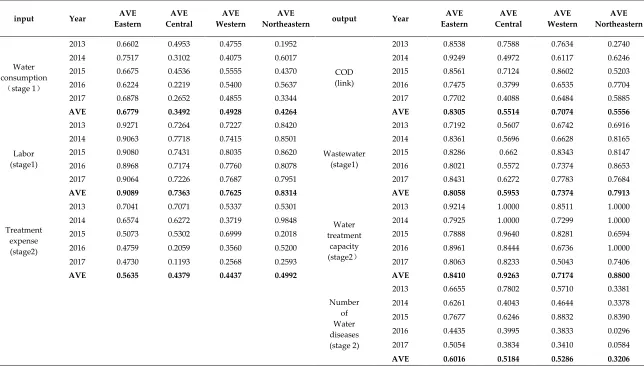
Table 3 lists the average efficiency values of wastewater and COD in four regions from 2013 to 2017. 34
The wastewater discharge efficiency of the eastern region is better than that of the other three regions, and 35
the wastewater discharge efficiency of the central region is the lowest among the four regions. 36
The average COD efficiency scores on the whole in northeast China rose the most and made the most 37
obvious progress. However, the average level was still not high and fluctuated significantly. The average 38
scores of COD efficiency in the eastern, central, and western regions decreased, especially in the central 39
region. In 2016, the average score of COD efficiency in the central region was only 0.3799. The average score 40
in the eastern region fell slightly, but was still the best of the four regions, followed by the west, with the 41
central region as the worst. 42
Table 3 presents the output efficiency score of Stage2 water diseases and water treatment capacity in 43
2013-2017. The efficiencies of water diseases in all four regions are on the decline. The efficiency of the 44
eastern region generally dropped and reached its lowest level in 2016, with an efficiency of only around 0.4. 45
The efficiency of water pollution in the central region also generally fell. From 2013 to 2014, its efficiency 46
declined the fastest, from 0.78 to 0.40 and then reached the lowest in 2017 at only 0.38. The western region 47
rose from 0.46 to 0.88 between 2014 and 2015, which was the best efficiency among the four regions for the 48
five years of statistics. In the northeastern region, the efficiency was basically stable in the first two years, 49
but it fluctuated greatly in the next three years, from 0.34 in 2014 to 0.84 in 2015. However, in 2016 and 2017, 50
the efficiency was only 0.03 and 0.06, which was greatly different from that before. 51
From the viewpoint of wastewater treatment efficiency, the eastern region has been in a stable state as 52
a whole, with efficiency sustained at around 0.8. The efficiency of the central region in 2013 and 2014 was 53
DEA-efficient, but there had been a slight decline since then. The western region as a whole was in a 54
trending decline, from the original level of 0.85 in 2013 to 0.50 in 2017. The overall efficiency of the northeast 55
region looks to be the best in all regions. The efficiencies of the first four years were DEA-efficient, but then 56
Table 3 The average scores of input and output variables in Stage1 and Stage2 from 2013-2017
input Year AVE Eastern
AVE Central
AVE Western
AVE
Northeastern output Year
AVE Eastern
AVE Central
AVE Western
AVE Northeastern
Water consumption
(stage 1)
2013 0.6602 0.4953 0.4755 0.1952
COD (link)
2013 0.8538 0.7588 0.7634 0.2740
2014 0.7517 0.3102 0.4075 0.6017 2014 0.9249 0.4972 0.6117 0.6246
2015 0.6675 0.4536 0.5555 0.4370 2015 0.8561 0.7124 0.8602 0.5203
2016 0.6224 0.2219 0.5400 0.5637 2016 0.7475 0.3799 0.6535 0.7704
2017 0.6878 0.2652 0.4855 0.3344 2017 0.7702 0.4088 0.6484 0.5885
AVE 0.6779 0.3492 0.4928 0.4264 AVE 0.8305 0.5514 0.7074 0.5556
Labor (stage1)
2013 0.9271 0.7264 0.7227 0.8420
Wastewater (stage1)
2013 0.7192 0.5607 0.6742 0.6916
2014 0.9063 0.7718 0.7415 0.8501 2014 0.8361 0.5696 0.6628 0.8165
2015 0.9080 0.7431 0.8035 0.8620 2015 0.8286 0.662 0.8343 0.8147
2016 0.8968 0.7174 0.7760 0.8078 2016 0.8021 0.5572 0.7374 0.8653
2017 0.9064 0.7226 0.7687 0.7951 2017 0.8431 0.6272 0.7783 0.7684
AVE 0.9089 0.7363 0.7625 0.8314 AVE 0.8058 0.5953 0.7374 0.7913
Treatment expense (stage2)
2013 0.7041 0.7071 0.5337 0.5301
Water treatment
capacity (stage2)
2013 0.9214 1.0000 0.8511 1.0000
2014 0.6574 0.6272 0.3719 0.9848 2014 0.7925 1.0000 0.7299 1.0000
2015 0.5073 0.5302 0.6999 0.2018 2015 0.7888 0.9640 0.8281 0.6594
2016 0.4759 0.2059 0.3560 0.5200 2016 0.8961 0.8444 0.6736 1.0000
2017 0.4730 0.1193 0.2568 0.2593 2017 0.8063 0.8233 0.5043 0.7406
AVE 0.5635 0.4379 0.4437 0.4992 AVE 0.8410 0.9263 0.7174 0.8800
Number of Water diseases (stage 2)
2013 0.6655 0.7802 0.5710 0.3381
2014 0.6261 0.4043 0.4644 0.3378
2015 0.7677 0.6246 0.8832 0.8390
2016 0.4435 0.3995 0.3833 0.0296
2017 0.5054 0.3834 0.3410 0.0584
1
2
Figure 5a. Input variables radar map from 2013 to 2017 3
4
5
Figure 5b. Output variables radar map from 2013 to 2017 6
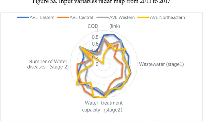
Figure 5a-5b shows the input and output variables radar map from 2013 to 2017. From Figure 5a, the 7
efficiency scores of the three input variables in the eastern region are better than those in the other three 8
regions, and the differences score of the variables in the eastern region are different. However, the efficiency 9
of input variables in the central, western and northeastern regions is great unbalanced. Among the three 10
input variables, the scores of labor efficiency are better than that of water consumption and treatment 11
expense. 12
From Figure 5b, the efficiency score of water treatment capacity of the four output variables is generally 13
better than the other three output variables and the four regions are all at a higher efficiency level. From a 14
regional perspective, there is strong correlation between COD efficiency score and water diseases, and the 15
efficiency of water diseases is relatively high in areas with high COD efficiency. Except for water treatment 16
capacity, the output variable efficiency in the eastern region is generally better than the other three regions. 17
There is still room for improvement in the central and northeastern regions. 18
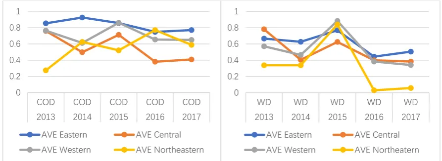
In order to clearly describe the correlation between COD and water diseases, Figure 6 was drawn to 19
analyze the specific values and changes of these two variables during 2013-2017. The efficiency values of 20
COD and water diseases showed basically the same fluctuation trend. Taking the central region as an 21
example, the efficiency of COD decreased from 0.7588 in 2013 to 0.4927 in 2014, and the efficiency of water 22
diseases also decreased from 0.7802 in 2013 to 0.4043 in 2014. Then the efficiency of COD increased from 23
0.4972 to 0.7124 from 2014 to 2015, correspondingly, the efficiency of water diseases also increased from 24
0.4043 in 2014 to 0.6246 in 2015. 25
0 0.2 0.4 0.6 0.8 1
Water consumption( stage 1)
Labor (stage1) Treatment expense
(stage2)
AVE Eastern AVE Central
AVE Western AVE Northeastern
0 0.2 0.4 0.6 0.8 1
COD (link)
Wastewater (stage1)
Water treatment capacity (stage2) Number of Water
diseases (stage 2)
26
Figure 6. COD and WD (water diseases) line charts from 2013 to 2017.
27
5. Conclusions and recommendations
28
5.1 Conclusion 29
From the perspective of total efficiency indicators, we offer the following conclusions. 30
(1) In addition to the increase in the average efficiency level in the northeastern region, the eastern, 31
western, and central regions showed a downward trend. The eastern region performed best overall. 32
(2) The cost-benefit of wastewater treatment investment in four regions has declined, and the central 33
region has the largest decline. The situation in Northeast China is similar to that in West China, and the 34
efficiency in most areas is further reduced. 35
(3) Wastewater discharge efficiency in the central region is at the lowest level in the past five years. 36
COD output fluctuates significantly, although the efficiency of the eastern region has declined, the efficiency 37
is still optimal. 38
(4) The efficiency of wastewater treatment is basically stable, and the efficiency of wastewater 39
treatment in Northeast China is the best. But the scores of the occurrence efficiency of water disasters in the 40
northeast region is the worst. 41
(5) The efficiency of prevention and control of water diseases in all four regions are declining. There is 42
a close relationship between COD and water diseases efficiency. In the central and western regions, there is 43
a positive correlation between the two scores. But the effect of COD efficiency on water health efficiency in 44
the eastern and northeastern regions is limited. 45
In summary, the overall situation in the eastern region is better than that in the central, western, and 46
northeastern regions. China has a vast amount of territory, a clear regional gap, a large economic gap, and 47
large differences in economic and social development. 48
5.2 Recommendations for the future. 49
According to the characteristics of each region, measures should be taken to suit local conditions, which 50
we present as follows. 51
1. Eastern region 52
From the comparison of the efficiencies of COD and water pollution diseases, it can be seen that the 53
former can improve the latter. Therefore, the eastern region should pay more attention to the control of 54
COD content and improve the requirements of corresponding indicators, so as to reduce the number of 55
water pollution diseases and achieve the goal of improving the overall efficiency. At the same time, due to 56
the limited natural purification capacity of the water resources, the eastern region should further adjust its 57
industrial structure and adopt measures such as shutting down, mergers and acquisitions, or 58
transformation for enterprises with large water consumption, heavy pollution, and high cost of pollution 59
control. Through a reasonable industrial layout to make full use of the ability of the natural environment, 60
0 0.2 0.4 0.6 0.8 1
COD COD COD COD COD
2013 2014 2015 2016 2017
AVE Eastern AVE Central
AVE Western AVE Northeastern
0 0.2 0.4 0.6 0.8 1
WD WD WD WD WD
2013 2014 2015 2016 2017
AVE Eastern AVE Central
the vicious circle can become a virtuous circle and thus play a role in developing the economy and 61
controlling pollution. 62
2. Central region 63
Since water efficiency in the central region is the lowest among the four regions, attention should be 64
paid to improving relevant technical policies and standards to improve water consumption efficiency. The 65
government should encourage enterprises to carry out technological transformation, promote clean 66
production, reduce water consumption per unit of product, and strengthen water reuse. In order to control 67
the development of water pollution, a more complete urban sewage treatment system needs to be 68
established, such as guiding industrial enterprises to actively control water pollution, especially the 69
separate disposal of toxic pollutants or pre-treatment. The centralized treatment of urban sewage can be 70
gradually realized through industrial layout, adjustments to urban layout and construction, and 71
improvements in urban sewer pipe networks, thus combining urban sewage treatment with industrial 72
wastewater treatment. 73
3. Western and Northeastern regions 74
The efficiency of wastewater treatment in the western and northeastern regions needs to be improved. 75
Therefore, the local governments should broaden the investment channels of urban wastewater 76
construction projects, apply for state-specific subsidies, and establish special wastewater treatment funds. 77
Wastewater treatment efficiency should be improved through effective and accurate wastewater treatment 78
inputs. Timely updated wastewater treatment systems and installations can also improve wastewater 79
utilization efficiency, enhance wastewater reusability, encourage reuse of wastewater, and reduce direct 80
and indirect discharges of wastewater. At the same time, the relevant authorities must pay attention to the 81
safety of wastewater reuse and avoid unnecessary harm to public health. 82
In the aspect of COD reduction and prevention and control of water diseases, the following measures 83
should be actively carried out. 84
(1) Strengthen water quality monitoring of upstream water sources and conduct regular water source 85
pollution surveys. Because of the strong correlation between COD and water pollution, water quality testing 86
and pollution control measures should be strengthened. Upstream monitoring can focus on and select 87
projects that have an impact on water quality. The sensory properties of water such as turbidity and odor, 88
organic matter pollution, eutrophication, and microbial indicators of bacterial contamination should be 89
targeted. At the same time, according to the type of water pollution, a regular survey can be conducted. The 90
water samples of sewage discharge ports must be entrusted to health and epidemic prevention or 91
environmental protection departments for analysis, and the survey results can then be compiled into 92
written materials to predict the trend of pollution development. 93
(2) Reduce and eliminate the amount of wastewater exceeding the standard of pollutants. First, a 94
reform process can be used to reduce or even eliminate wastewater or to decrease the toxicity of wastewater. 95
Second, wastewater must be reused and repeated water and circulating water systems must be utilized as 96
much as possible to minimize wastewater discharge or to recycle the production wastewater after proper 97
treatment. At the same time, the government should establish a scientific charging mechanism for urban 98
water and wastewater treatment and use pricing policies to jointly adjust the demand for drainage and to 99
reduce the amount of sewage. 100
(3) Govern pollution sources according to law. The prevention and control of water pollution highly 101
correlate to the health of residents, have far-reaching effects, and must be regulated and guaranteed through 102
laws. Polluting entities that have affected the quality of water resources must be treated according to laws 103
that rely on closely coordinated management among central and local governments, environmental 104
protection, and health departments. At the same time, related organizations can strengthen media publicity 105
and guidance, enhance public water source protection and wastewater reuse awareness, and pay attention 106
to the health problems and their root causes brought about by wastewater discharge. 107
Author Contributions: conceptualization, Y-N.S and F-R.R.; methodology, F-R.R.; software, F-R.R.; validation, Y-N.S
108
and F-R.R.; formal analysis, J-W.L; investigation, N-X.S; resources, Y-N.S; data curation, F-R.R.; writing—original draft
109
preparation, Y-N.S; writing—review and editing, J-W.L; visualization, Y-N.S; supervision, J-W.L; project
110
administration, F-R.R.; funding acquisition, Y-N.S.