Christophe Pfeifer1,2 and Patrick Haddad3 1
Karlsruhe Institute of Technology, Karlsruhe, Germany 2
Grenoble INP - Ensimag, Grenoble, France
3
STMicroelectronics SA, Rousset, France
Abstract. Recent publications, such as [10] and [13], exploit the advan-tages of deep-learning techniques in performing Side-Channel Attacks. One example of the Side-Channel community interest for such techniques is the release of the public ASCAD database, which provides power con-sumption traces of a masked 128-bit AES implementation, and is meant to be a common benchmark to compare deep-learning techniques perfor-mances. In this paper, we propose two ways of improving the effectiveness of such attacks. The first one is as new kind of layer for neural networks, called “Spread” layer, which is efficient at tackling side-channel attacks issues, since it reduces the number of layers required and speeds up the learning phase. Our second proposal is an efficient way to correct the neural network predictions, based on its confusion matrix. We have vali-dated both methods on ASCAD database, and conclude that they reduce the number of traces required to succeed attacks. In this article, we show their effectiveness for first-order and second-order attacks.
Keywords: Deep-learning·Side-Channel Attack · Spread layer· AS-CAD·Confusion matrix·Bayesian correction.
1
Introduction
1.1 Side-channel attacks
Side-channel attacks are a set of attack methods used to target cryptographic devices and retrieve sensitive information. These methods may leverage power consumption traces gathered when executing an algorithm.
Classes of side-channel attacks These attacks may work according to two sce-narios: profiled or non-profiled.
– In the profiled case, the attacker possesses a device similar to the one being targeted and acquires beforehand many execution traces according to dif-ferent parameters. Based on these observations, he elaborates and tunes a model able to retrieve the sensitive information targeted. This category of attacks includes Templates Attacks [4] and Stochastic models (a.k.a Linear Regression Analysis) [5, 12, 11].
– In the non-profiled case, the attacker does not have such a device at his disposal. This set of non-profiled attacks includes, among others, Differential Power Analysis [14], Correlation Power Analysis [8] and Mutual Information Analysis [6, 3].
In both scenarios, the adversary obtains afterwards attack traces and shall re-trieve some sensitive information used. In addition, he may know some public information such as the the plaintext, the ciphertext, etc.
1.2 Deep-learning
Some models used to predict sensitive data rely on deep-learning, which is a branch of machine learning, namely methods learning how to extract relevant information out of a usually large amount of data, without being explicitly told how to. Deep-learning is specifically based on the use of neural networks to make predictions. The basis component of a neural network is the neuron, which performs a single operation on its input(s). Neurons are assembled into layers, which are then stacked.
Architecture Some common layers used in deep-learning are the following:
– Dense layers are composed of many neurons, whose inputs are connected to all outputs of the previous layer. Each input is then multiplied by some trainable weights, and summed up before being passed to the next layer.
– Activation layers are used to increase the computational capacity of the network. They implement an activation function, which is applied to each output of the previous layer, and whose results make the output of the layer. Such functions may be non-linear or almost everywhere differentiable and are usually not trainable. For instance, the softmax function (a special case of activation functions since it is applied on the whole previous layer) is used to obtain a probability distribution out of its input.
A network exclusively made of the two aforementioned types of layers is called a Multi-Layer Perceptron (MLP).
ments:
– Atraining setcontains observations, for which the correct output labels (e.g. the value of the targeted data) are known. it is used before the attack to train and tune the neural network.
– Avalidation set contains observations, whose correct labels are also known, but which are not used for the training. They serve as a token to prevent lack of generality (called “overfitting”). The accuracy of the neural network predictions on these data is regularly verified and the learning process may be stopped if a decrease occurs.
– Aloss function is applied to measure the inconsistency between the predic-tions and the expected labels.
– An optimization algorithm is then applied on the network to tune the train-able weights in order to reduce the loss function.
The neural network loops through the training set many times (many “epochs”) to optimize its weights. Since this set may be very large, it is chunked into small batches of observations, which are then processed simultaneously (e.g. taking advantage of GPU). After each epoch, we monitor the accuracy of the predictions on the training and validation set. At the end of the learning phase, a confusion matrix, showing the distribution of the predicted classes for a given true label, can be computed so as to visualize which classes are correctly predicted and which ones are not.
Application to side-channel attacks Deep-learning models may be used to retrieve sensitive data in profiled or non-profiled contexts. In the former, one way to adapt the problem to their usage is to give the power consumption traces directly as input for the neural network to learn. The targeted labels are not necessarily the raw sensitive data, but may be the result of a leakage model function applied to them. A common choice is the use of the Hamming weight function.
1.3 Related works
Side-channel attacks based on deep-learning is still a recent research field but some works have already been published.
Advanced Encryption Standard The AES is a encryption algorithm using the same key for both encryption and decryption (i.e. symmetric). This algorithm manipulates the following data:
– A plaintext, which is the message being encrypted. It has a length of 128 bits.
– A ciphertext, which is the resulting encrypted message. It has also a length of 128 bits.
– A secret key, which is used to encrypt the plaintext. This key is a sensitive data and has also a length of 128 bits in the case of the ASCAD database. During the AES execution, some internal variables are correlated to the power consumption. One of the operations executed is a non-linear byte substitution, called aSbox. In the case of a 128-bit AES, the first time this operation is done, it is applied to all bytes of the plaintext, performing the following operation:
S=Sbox(plaintext byte⊕key byte)
where (S, plaintext byte, key byte)∈J0,255K3 (1) The substitution table being known and reversible,Sis a sensitive data because it depends on the secret key. Since the plaintext may be known by the attacker, he may retrieve the secret key with a first-order attack.
Masking In order to prevent such attacks, countermeasures are implemented. In ASCAD database, a 8-bit random mask is applied to the output of the Sbox:
S =Sbox(plaintext byte⊕key byte)⊕M
where M ∈J0,255K (2)
This increases by one the order of the attack required to retrieve the key. One shall know the maskM and the masked Sbox outputSso as to retrieve the key byte.
In this article, we compare the performances of the best MLP proposed in [10] to our solution. The Signal-to-Noise ratio of the sensitive data in these traces has been discussed in [10].
First of all, we introduce in Section 2 a new layer called “Spread”, which im-proves greatly the performance of first-order side-channel attacks based on neural networks, compared to the ASCAD best MLP. Then, in Section 3, we extend this kind of attack to second-order attacks. Eventually, we propose in Section 4 a Bayesian correction of the neural network predictions, which reduces even more the number of attack traces required.
2
First-order attack
2.1 Adversary strength
In this model, as summarized in Figure 1, the adversary has at his disposal a similar device to the one being attacked, and can run it a given amount of times during a training phase. At each run, he varies the plaintext and acquires the corresponding consumption trace. In this scenario, the adversary can not change the key, but knows its value and is also able to read the ciphertexts.
After that, during a so called attack phase, the targeted device may be run a given amount of times. At each run, the adversary may change the plaintext and acquires the attack trace with its respective ciphertext. The goal is to retrieve the key used by the device under attack. This is the same attack model as in ASCAD publication [10].
Profiled Training phase
AES
provides Traces Plaintexts Ciphertexts Keys
Attack phase
Traces, Plaintexts, Ciphertexts →Retrieve key
Fig. 1: Attack context.
2.2 Protocol
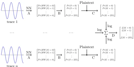
available device. After that, the second phase of our protocol relies on the Max-imum Likelihood Estimator (MLE). First (step A), we apply the trained neural network to each attack trace, so as to obtain a probability vector of the Hamming weight of the Sbox output value. Then (step B), knowing the Hamming weight distribution and assuming that the Sbox outputs are uniformly distributed over all possible byte values, we compute the probability for each Sbox output byte to be the correct one, using Equation 3.
P r(S=s) =P r(HW(S) =HW(s))
C8HW(s)
(3)
where P r(HW(S) = HW(s)) is given by our neural network (step A). After-wards (step C), these probabilities can be used to derive probabilities over the keys, since one Sbox output and one plaintext match exactly one key byte, as recalled in Equation 4.
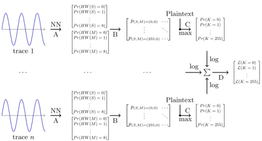
key byte=Sbox−1(S)⊕plaintext byte (4) Eventually (step D), the sum of the logarithm of each key hypothesis proba-bility over all attack traces gives us the likelihood of each key. The higher the likelihood, the more likely is one key hypothesis. The entire recombination pro-cess is summarized in Figure 2 and the algorithm is described, step by step, in Algorithm 1.
Design choice We decided to implement the Maximum Likelihood Estimator (MLE) to combine together the probability vectors of each attack trace, since it has two interesting properties, according to [7]:
– The MLE is the best estimator asymptotically. This means that it has the best convergence rate when the number of traces increases.
– The MLE is consistent under appropriate conditions. Therefore, it should converge to the true value when the number of traces increases.
More details about these conditions may be found in [7].
Given this protocol, the neural network predictions play a determining role in the key retrieval process. In the following two subsections, we give more details about its implementation and specifically about the new layer, called Spread layer, which we devised.
2.3 Spread layer
trace 1 NN A
P r(HW(S) = 0)
P r(HW(S) = 1) . . .
P r(HW(S) = 8)
B
P r(S= 0)
P r(S= 1) . . .
P r(S= 255)
C Plaintext
P r(K= 0)
P r(K= 1) . . .
P r(K= 255)
. . . . tracen NN A
P r(HW(S) = 0)
P r(HW(S) = 1) . . .
P r(HW(S) = 8)
B
P r(S= 0)
P r(S= 1) . . .
P r(S= 255)
C Plaintext
P r(K= 0)
P r(K= 1) . . .
P r(K= 255)
log log log P D
L(K= 0)
L(K= 1) . . .
L(K= 255)
Fig. 2: Recombination of attack traces for the first-order attack.
Algorithm 1: Secret key byte retrieval for the first-order attack. Input:traces: Attack traces
Input:N N: Neural network giving prob. vect. for HW(Sbox byte) Output:Secret key byte
fortrace∈tracesdo
A probSboxHW[]←N N(trace); fors∈All(Sbox bytes)do
B probM atrix[s]←probSboxHW[HW(s)]
CHW8 (s) ;
end
fors∈All(Sbox bytes)do
C vn[Sbox−1(s)⊕ptxt]←probM atrix[s]; end
D v←v+log(vn); end
classification is the activation layer, because its non-regularity can be used to have a very different response according to the input value. For instance, a binary step, having 0 or 1 as output if its input is respectively negative or positive, will efficiently discriminate 2 values, which have been centered around zero. But in our case, we want to discriminate between all possible Hamming weights. The Spread layer is intended to perform this operation more efficiently. The basic idea is to transform the output of a neuron into a spatially-encoded information at the expense of a dimensionality increase, since the latter is known to be efficiently handled by neural networks. We implemented it directly using Tensorflow (and not Keras backend, which lacks some functions at the time of this writing).
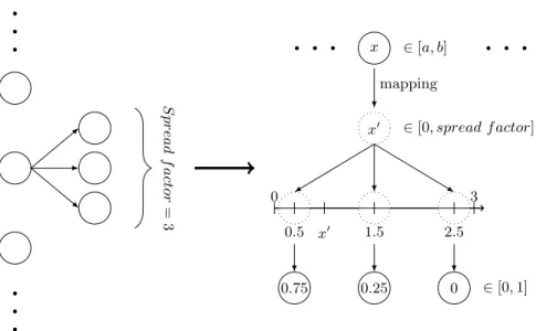
Implementation details As described in Figure 3, the Spread layer extends the dimension of the previous layer by aspread f actor, its only hyperparameter. Each new neuron created is related to a neuron of the previous layer and is assigned a centroid from 0.5 to spread f actor - 0.5. When a valuex is passed as input by the previous neuron, this value is remapped linearly in the interval [0,spread f actor] to a new valuex0. Then, the 1 or 2 neurons, whose centroids are the closest tox0, output a value proportional to their distance to x0, more precisely:
∀x0∈[0, spread f actor],∀neuronnc with centroidc,
nc(x0) =
1 ifc= 0.5∧x0< c
1 ifc=spread f actor−0.5∧x0 > c max(0,1−abs(c−x0)) otherwise
(5)
Behavior The Spread layer outputs values belonging to [0,1], whose sum per input neuron always equals one. Most of the time, 2 neurons have a non-zero output per input neuron, except when one has a value equal to 1, which occurs either when the input exactly matches a centroid, or when the output saturates at the borders.
The training phase consists in learning the minimum and maximum output values of each input neuron, in order to map x without saturation. Due to implementation constraints, the initial interval is [0,1] and the previous layer shall output at least over this interval for better fitting. But this is the case most of the time with the usual initializers.
In the next subsections, we describe how we implemented the spread layer in a neural network.
2.4 Neural network structure
..
.
..
.
S
pr
ead
f
actor
=
3
x ∈[a, b]
. . .
. . .
mapping
x0 ∈[0, spread f actor]
0 3
0.5 x0 1.5 2.5
0.75 0.25 0 ∈[0,1]
Fig. 3: Spread layer principle with example spread factor of 3.
“None”, but equals to 100 for all our tests.
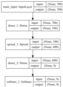
It has been trained to predict the Hamming weight of the Sbox output, that is:
y=HammingW eight(Sbox(plaintext⊕key)) (6) It has been compiled using the Nadam optimizer and the categorical crossentropy loss function. At the beginning of this section, we presented the protocol used to retrieve the key and the way we implemented the neural network. In the next two sections, we evaluate and compare our proposed improvement to state-of-the-art results.
2.5 Validation
main_input: InputLayer input: output:
(None, 700)
(None, 700)
dense_1: Dense input: output:
(None, 700)
(None, 100)
spread_1: Spread input: output:
(None, 100)
(None, 600)
dense_2: Dense input: output:
(None, 600)
(None, 9)
softmax_1: Softmax input: output:
(None, 9)
(None, 9)
Fig. 4: Architecture of theSpread & HW neural network.
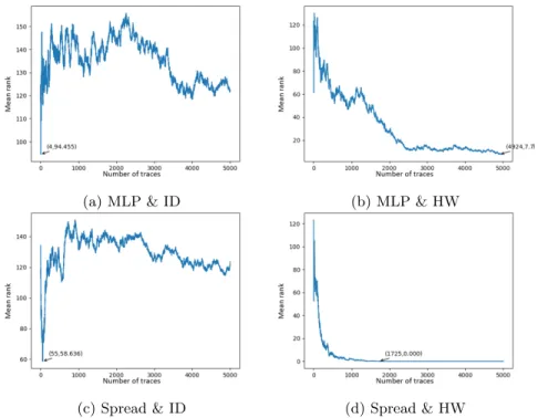
We then performed the attack on subsets of remaining ASCAD traces. Each subset contains 5,000 attack traces. We computed the mean rank of the correct key byte over all attacks, and considered the attack as a success (PASS) if all the attacks on subsets succeeded within less than 5,000 attack traces; that is, that the correct key byte is the most likely (i.e. has rank 0) at some points and keeps its rank until the end of our subset. We indicated in brackets the minimal amount of traces required such that all attacks succeed.
On the other hand, we considered the attack a failure (FAIL) if any of our at-tacks did not lead to the correct key byte in the end, in which case we indicate the amount of succeeded attacks divided by the amount of total attacks.
In practice, the labels do not match those of Equation 6, but also take into account the mask values. As we know them during the attack phase, this is equiv-alent to a first-order AES implementation, and is what has been done in [10].
2.6 Results and comparisons
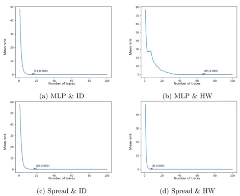
training set too, and decided to lower the attack set size to 100 traces, in order to compute our mean over 100 attack sets, as shown in Figure 6. In this case, MLP & ID andSpread & ID have similar results. As already stated in [10], we can verify thatMLP & HW is much worse thanMLP & ID. ButSpread & HW shows impressive results by requiring for its worst-case attack less than half of the traces needed by the worst-case MLP & ID attack.
(a) MLP & ID (b) MLP & HW
(c) Spread & ID (d) Spread & HW
Fig. 5: Mean rank of the correct key byte as a function of number of attack traces, given 1,000 training traces.
Table 1 compares all four combinations for various amounts of training traces.
2.7 Conclusion
(a) MLP & ID (b) MLP & HW
(c) Spread & ID (d) Spread & HW
Fig. 6: Mean rank of the correct key byte as a function of number of attack traces, given 50,000 training traces.
Table 1: Comparison of all four networks according to the amount of training traces.
Nb of training traces 1,000 2,000 4,000 8,000 MLP & ID (ASCAD) FAIL (0/11) FAIL (0/11) FAIL (0/11) FAIL (1/10)
MLP & HW FAIL (2/11) FAIL (9/11) FAIL (1/11) PASS (230) Spread & ID FAIL (0/11) FAIL (0/11) FAIL (7/11) PASS (100) Spread & HW PASS (1302) PASS (116) PASS (35) PASS (13) Nb of training traces 16,000 32,000 50,000
used for the profiling phase, usually implement counters, limiting the number of consumption traces, which can be acquired. Encouraged by the promising results obtained in Section 2, we decided to adapt this first-order attack protocol to a second-order attack.
3
Second-order attack
3.1 Adversary strength
In this model, the adversary has at his disposal a similar device as the one being attacked. During the training phase, he can vary the plaintexts and the masks used a given amount of times, and acquires the consumption traces as well as the ciphertexts. The key is fixed but known to him.
During the attack phase, the adversary can run the attacked device a given amount of times, may change the plaintexts, but knows neither the masks, nor the key. The adversary’s goal is to retrieve this latter key.
3.2 Protocol
Here, we adapted the previously used protocol to the case, where we know nei-ther the Sbox output, nor the mask. First (step A), we apply a trained neural network on each of our attack traces, so as to obtain a probability vector of the Hamming weights of the masked Sbox output value and of the mask. Then (step B), knowing the Hamming weight distribution and assuming that the keys and the masks are uniformly distributed over all possible byte values, we compute the probability for each couple (M ask byte, M asked Sbox byte) to be the cor-rect one, using Equation 7. This is justified by the fact that the Sbox output and the mask are independent random variables when the key is unknown.
P r(M ask byte=m∩Sbox byte=s) = probM ask[m]·probSbox[s]
C8HW(m)·C8HW(s)
(7)
Afterwards (step C), these probabilities can be used to derive probabilities over the keys. Since one couple and one plaintext match exactly one key byte, as re-called in Equation 8, we keep the maximum probability associated to all couples implying the same given key.
trace 1 NN A
P r(HW(S) = 0)
P r(HW(S) = 1) . . .
P r(HW(S) = 8)
P r(HW(M) = 0)
P r(HW(M) = 1) . . .
P r(HW(M) = 8)
B
p(S,M)=(0,0) . . . . . . . ..
p(S,M)=(255,0). . .
max C Plaintext
P r(K= 0)
P r(K= 1) . . .
P r(K= 255)
. . . . tracen NN A
P r(HW(S) = 0)
P r(HW(S) = 1) . . .
P r(HW(S) = 8)
P r(HW(M) = 0)
P r(HW(M) = 1) . . .
P r(HW(M) = 8)
B
p(S,M)=(0,0) . . . . . . . ..
p(S,M)=(255,0). . .
max C Plaintext
P r(K= 0)
P r(K= 1) . . .
P r(K= 255)
log log log P D
L(K= 0)
L(K= 1) . . .
L(K= 255)
Fig. 7: Recombination of attack traces for the second-order attack.
Algorithm 2: Secret key byte retrieval for the second-order attack. Input:traces: Attack traces
Input:N N: Neural network giving prob. vect. for HW(Mask byte) and HW(Sbox byte)
Output:Secret key byte fortrace∈tracesdo
A probM ask[],probSbox[]←N N(trace);
for(m, s)∈AllCouples(M ask bytes, Sbox bytes)do
B probM atrix[m, s]← probM ask[m]·probSbox[s]
C8HW(m)·C8HW(s) ;
end
forkey byte∈All(Key bytes)do
C vn[key byte]←max(m,s),key byte=Sbox−1(s⊕m)⊕ptxt(probM atrix[m, s]);
end
D v←v+log(vn);
end
couples of Mask and Sbox for the following reason. We may model the choice of the correct key byte k as 28 statistical hypothesis tests like this: the null hypothesis is “k is the correct key” and the other alternative is “k is not the correct key”. Then, we want to minimize the risk to reject the null hypothesis when this one appears to be true (also called minimizing the Type-I error) at the expense of requiring more attack traces. Keeping the maximal probability minimizes this kind of error.
3.3 Architecture of our neural network
Our neural network has been designed with two branches. The first one is trained to predict the Hamming weight of the masked Sbox output. The other one is intended to predict the Hamming weight of the mask applied, which is also to be found in the consumption traces. This architecture is depicted in Figure 8. We altered the MLP best from ASCAD the same way, adding a branch for each sensitive data we want to retrieve. The compilation parameters have not been changed.
3.4 Results
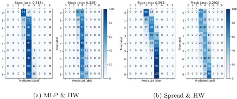
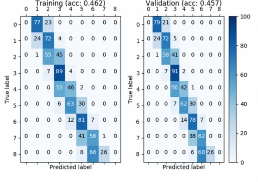
Behavior comparison In Figure 9, we depicted the confusion matrices of the two branches for the MLP & HW and the Spread & HW trained with 2,000 training traces. Two different behaviors can be noticed. On the one hand, the MLP & HW tends to predict the most represented label first, and then to grasp the more distant labels. On the other hand, theSpread & HW best predicts labels around the most represented one, which leads to a slightly lesser accuracy. Nevertheless, this is of no use for the secret key retrieval algorithm to have only the most represented label predicted. Rather than that, we would like to have at least two distinct labels with accurate enough predictions. A way to represent that is to compute the Pearson correlation coefficient of the confusion matrix. If it has a high absolute value, then the predictions are linearly correlated to the true labels, and we can use these for our algorithm. But if the predictions do not depend on the true label, the coefficient will be near to zero. And indeed, we observe in Figure 10 that this coefficient is higher for theSpread & HW neural networks, which leads to the success of all attacks, compared to the other one, having no successful attack at all.
main_input: InputLayer input: output:
(None, 700, 1)
(None, 700, 1)
flattenSbox: Flatten input: output:
(None, 700, 1)
(None, 700) flattenMask: Flatten input:
output:
(None, 700, 1)
(None, 700)
denseSbox0: Dense input: output:
(None, 700)
(None, 100) denseMask0: Dense input:
output:
(None, 700)
(None, 100)
spreadSbox0: Spread input: output:
(None, 100)
(None, 600) spreadMask0: Spread input:
output:
(None, 100)
(None, 600)
denseSbox1: Dense input: output:
(None, 600)
(None, 9) denseMask1: Dense input:
output:
(None, 600)
(None, 9)
sbox_output: Softmax input: output:
(None, 9)
(None, 9) mask_output: Softmax input:
output:
(None, 9)
(None, 9)
Fig. 8: Architecture of theSpread & HW neural network with two branches.
(a) MLP & HW (b) Spread & HW
(a) MLP & HW (b) Spread & HW
Fig. 10: Comparison of Pearson correlation coefficient according to the number of epochs in the second-order attack case with 2,000 training traces.
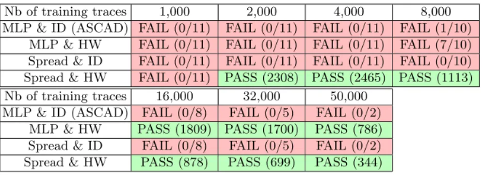
Table 2: Comparison of all four networks according to the amount of training traces.
Nb of training traces 1,000 2,000 4,000 8,000 MLP & ID (ASCAD) FAIL (0/11) FAIL (0/11) FAIL (0/11) FAIL (1/10)
MLP & HW FAIL (0/11) FAIL (0/11) FAIL (0/11) FAIL (7/10) Spread & ID FAIL (0/11) FAIL (0/11) FAIL (0/11) FAIL (0/10) Spread & HW FAIL (0/11) PASS (2308) PASS (2465) PASS (1113) Nb of training traces 16,000 32,000 50,000
3.5 Conclusion
Similarly to what we have seen in Section 2 for first-order attacks, we observed here that the use of our Spread layer-based network also shows better results regarding the number of attack traces required for second-order attacks. More-over, our improvement allows successful attacks with a small number of available training traces and improves the convergence speed towards the correct key byte. In the next section, we introduce the last improvement of this article. It reduces the number of attack traces required. As it relies on the confusion matrix and Bayes’ theorem, we call it theBayesian correction.
4
Bayesian correction
The use of confusion matrices to provide information on the errors and improve the accuracy has already been studied, among others, in [2, 1, 9, 15]. Here, we adapted these approaches to our case.
4.1 Principle
The confusion matrix gives us valuable information about the bias and variance of the neural network for each input label. We decided to leverage it in order to correct the predictions. Indeed, its output may be considered as a random variable Y, whose value depends on the expected label, a random variable X. The confusion matrix let us know the distribution of Y knowing X, that is
P r(Y|X). By means of Bayes’ theorem, which is recalled in Equation 9, we can retrieve the probability of the true label knowing the output of the neural network, that is P r(X|Y) and thus correct somewhat its predictions.
P r(X|Y) =P r(Y|X)·P r(X)
P r(Y) (9)
In the case of the Hamming weight leakage model,X follows a binomial distri-bution. More precisely,X ∼ B(8,12) and the distribution of Y is known thanks to the law of total probability. The final formula is summarized in Equation 10.
P r(X|Y =y) = P r(Y =y|X)·P r(X)
P8
x=0P r(Y =y|X=x)·P r(X =x)
(10)
4.2 Results
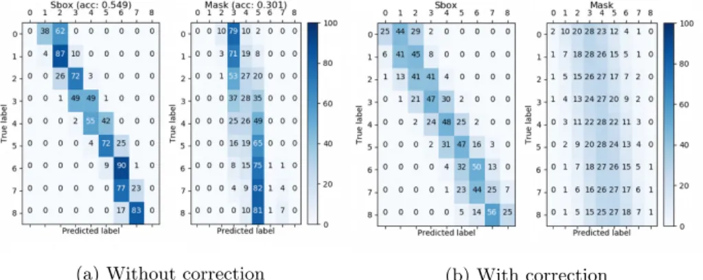
We compared the mean ranks of the correct key byte with and without correction for the same trainedSpread & HW neural network. Figure 12 shows the confusion matrices with and without this correction in the second-order attack. We notice that the correction enables better predictions of some Hamming weights with a few samples (e.g. labels 0 and 8). On the other hand, the mask predictions, which were strongly biased, become very fuzzy. Their respective correct key byte mean ranks are depicted in Figure 13. The results are worse than expected. It seems that a biased estimator is better than a corrected one in the case of a fuzzy confusion matrix, due to the presence of “columns” in the original confusion matrix, that is subgroups ofX values for which the distribution ofY is almost independent. The correction is not working great in this case, and even though our neural network is biased, the amount of required traces will be lower without correction, since it is more accurate over the most represented classes. Therefore, we decided to correct only the Sbox predictions.
(a) Without correction (b) With correction
Fig. 12: Confusion matrices ofSpread & HW trained on 16,000 training traces.
First-order attack scenario Table 3 compares the effect of the correction in the first-order attack case. The failure of the improvement on 1,000 training traces is due to the neural network inclination to predict the most represented labels and thus having a low Pearson correlation coefficient, as depicted in Fig-ure 14.
(a) Without correction (b) With correction
Fig. 13: Mean rank of correct key byte over 5 attacks.
Table 3: Comparison ofSpread & HW without and with correction. Nb of training traces 1,000 2,000 4,000 8,000
Spread & HW PASS (1302) PASS (138) PASS (44) PASS (18) Spread & HW & Correction FAIL (2/11) PASS (57) PASS (23) PASS (9)
Nb of training traces 16,000 32,000 50,000 Spread & HW PASS (8) PASS (8) PASS (6) Spread & HW & Correction PASS (8) PASS (7) PASS (5)
(a) Confusion matrix (b) Pearson correlation coefficient
Fig. 14: Metrics of Spread & HW trained with 1,000 traces in the first-order attack scenario.
Table 4: Comparison ofSpread & HW without and with correction. Nb of training traces 4,000 8,000 16,000 32,000
Spread & HW PASS (2465) PASS (1237) PASS (1305) PASS (1205) Spread & HW & Correction PASS (2272) PASS (947) PASS (1042) PASS (556)
4.3 Conclusion
The Bayesian correction of theSpread & HW predictions enables all our attacks to succeed with even less attack traces, by reducing this amount of up to more than 50%. Unfortunately, this method does not succeed when the output of the neural network is almost independent of its input. In such cases, it seems better to have few variances on the most represented labels, rather than to make the confusion matrix fuzzy. This is why we decided to correct only the Sbox predictions for the second-order attack.
5
Conclusion and perspectives
In this paper, we propose two different improvements, which increase the effec-tiveness of profiled side-channel attacks based on deep-learning techniques.
The first improvement is a new neural network layer, called Spread layer. Its goal is to reduce the amount of both training and attack traces required to retrieve the key. In order to evaluate the level of this reduction with the state-of-the-art neural network used for side-channel attacks, we followed the benchmark strategy promoted in [10]. The result of this evaluation confirms that the goal of the Spread layer has been achieved for first-order attacks as well as for second-order attacks.
The second improvement is a method of correcting the neural network predic-tions. It reduces most of the time even more the number of attack traces required to succeed the key retrieval.
Our new layer might be useful for other applications in the field of deep-learning, when one needs to perform a classification relying on the values of some input features. Indeed, the resulting neural network might be shallower than these based on the common activation layers.
Future works may be to assess our method with higher-order masking. In this case, the neural network would have one branch per share and the post-processing algorithm would comprise a matrix with more dimensions. Another possibility is to lower the hypothesis so as to target traces without mask knowl-edge.
Acknowledgment
1. 5th IIAI International Congress on Advanced Applied Informatics, IIAI-AAI 2016, Kumamoto, Japan, July 10-14, 2016. IEEE (2016), http://ieeexplore.ieee.org/xpl/mostRecentIssue.jsp?punumber=7557346
2. 20th International Conference on Information Fusion, FU-SION 2017, Xi’an, China, July 10-13, 2017. IEEE (2017), http://ieeexplore.ieee.org/xpl/mostRecentIssue.jsp?punumber=8002854
3. Batina, L., Gierlichs, B., Prouff, E., Rivain, M., Standaert, F., Veyrat-Charvillon, N.: Mutual information analysis: a comprehensive study. J. Cryptology 24(2), 269–291 (2011). https://doi.org/10.1007/s00145-010-9084-8, https://doi.org/10.1007/s00145-010-9084-8
4. Chari, S., Rao, J.R., Rohatgi, P.: Template attacks. In: Jr., B.S.K., Ko¸c, C¸ .K., Paar, C. (eds.) Cryptographic Hardware and Embedded Systems - CHES 2002, 4th International Workshop, Redwood Shores, CA, USA, August 13-15, 2002, Re-vised Papers. Lecture Notes in Computer Science, vol. 2523, pp. 13–28. Springer (2002). 36400-5 3, https://doi.org/10.1007/3-540-36400-5 3
5. Doget, J., Prouff, E., Rivain, M., Standaert, F.: Univariate side channel at-tacks and leakage modeling. IACR Cryptology ePrint Archive2011, 302 (2011), http://eprint.iacr.org/2011/302
6. Gierlichs, B., Batina, L., Preneel, B., Verbauwhede, I.: Revisiting higher-order DPA attacks: Multivariate mutual information analysis. IACR Cryptology ePrint Archive2009, 228 (2009), http://eprint.iacr.org/2009/228
7. Goodfellow, I., Bengio, Y., Courville, A.: Deep Learning. MIT Press (2016), http://www.deeplearningbook.org
8. Joye, M., Quisquater, J. (eds.): Cryptographic Hardware and Embedded Systems - CHES 2004: 6th International Workshop Cambridge, MA, USA, August 11-13, 2004. Proceedings, Lecture Notes in Computer Science, vol. 3156. Springer (2004). https://doi.org/10.1007/b99451, https://doi.org/10.1007/b99451
9. Leijon, L., Henter, G.E., Dahlquist, M.: Bayesian analysis of phoneme confusion matrices. IEEE/ACM Trans. Audio, Speech & Language Pro-cessing 24(3), 469–482 (2016). https://doi.org/10.1109/TASLP.2015.2512039, https://doi.org/10.1109/TASLP.2015.2512039
10. Prouff, E., Strullu, R., Benadjila, R., Cagli, E., Dumas, C.: Study of deep learning techniques for side-channel analysis and introduction to ASCAD database. IACR Cryptology ePrint Archive2018, 53 (2018), http://eprint.iacr.org/2018/053 11. Rao, J.R., Sunar, B. (eds.): Cryptographic Hardware and Embedded Systems
-CHES 2005, 7th International Workshop, Edinburgh, UK, August 29 - Septem-ber 1, 2005, Proceedings, Lecture Notes in Computer Science, vol. 3659. Springer (2005). https://doi.org/10.1007/11545262, https://doi.org/10.1007/11545262 12. Schindler, W.: Advanced stochastic methods in side channel analysis
on block ciphers in the presence of masking. J. Mathematical Cryp-tology 2(3), 291–310 (2008). https://doi.org/10.1515/JMC.2008.013, https://doi.org/10.1515/JMC.2008.013
13. Timon, B.: Non-profiled deep learning-based side-channel attacks. IACR Cryptol-ogy ePrint Archive2018, 196 (2018), http://eprint.iacr.org/2018/196