arXiv:1712.06239v1 [quant-ph] 18 Dec 2017
Quantum Algorithms for Boolean Equation Solving
and Quantum Algebraic Attack on Cryptosystems
Yu-Ao Chen1,2 and Xiao-Shan Gao1,2
1KLMM, Academy of Mathematics and Systems Science
Chinese Academy of Sciences, Beijing 100190, China
2University of Chinese Academy of Sciences, Beijing 100049, China
Email: [email protected]
December 19, 2017
Abstract
Decision of whether a Boolean equation system has a solution is an NPC problem and finding a solution is NP hard. In this paper, we present a quantum algorithm to decide whether a Boolean equation systemF has a solution and compute one if F does have solutions with any given success probability. The complexity of the algorithm is polynomial in the size of F and the condition number ofF. As a consequence, we have achieved exponential speedup for solving sparse Boolean equation systems if their condition numbers are small. We apply the quantum algorithm to the cryptanalysis of the stream cipher Trivum, the block cipher AES, the hash function SHA-3/Keccak, and the multivariate public key cryptosystems, and show that they are secure under quantum algebraic attack only if the condition numbers of the corresponding equation systems are large.
Keywords. Quantum algorithm, Boolean equation solving, polynomial system solving, HHL algorithm, condition number, stream cipher Trivum, block cipher AES, hash function SHA-3/Keccak, MPKC, 3-SAT, graph isomorphism.
1
Introduction
Solving Boolean equations is a fundamental problem in theoretical computer science. Decision of whether a Boolean equation system has a solution is an NPC problem and finding a solution is NP hard. On the other hand, finding a polynomial-time quantum algorithm for an NPC problem is a basic issue in quantum computing. In this paper, a quantum algorithm for Boolean equation solving will be given, which can be as much as exponentially faster than traditional algorithms for the same task under certain conditions.
1.1 Main results
Let F = {f1, . . . , fr} be a set of Boolean polynomials in variables X = {x1, . . . , xn} and with
total sparseness T =Pri=1#fi, where #fi is the number of terms in fi. Then, we have
As a consequence, we can solve Boolean equation systems using quantum computers with any given success probability and in polynomial-time if the condition number κ of F and the sparsenessT ofF are small, say whenκandT are poly(n). SinceT is the size of the input to the algorithm, it should be small for practical problems. For instance, all the equation systems from cryptanalysis in Section 6 are very sparse. Therefore, the key factor is the condition number. As a consequence, we have achieved exponential speedup for sparse Boolean equation solving if its condition number is small.
LetF ={f1, . . . , fr} ⊂C[X] be a set of polynomials inXwith total sparsenessT =Pri=1#fi
andǫ∈(0,1). A solutionaforF = 0 is called Boolean, if each coordinate ofais 0 or 1. Clearly, deciding whether F has a Boolean solution is NPC. We also give a quantum algorithm to compute Boolean solutions of F.
Theorem 1.2. There is a quantum algorithm which decides whether F = 0 has a Boolean solution and computes one if F = 0 does have Boolean solutions, with probability at least 1−ǫ
and complexity Oe(n2.5(n+T)κ2log 1/ǫ), where κ is the condition number of the polynomial system F (refer to Theorem 4.3 for definition).
We apply Theorem 1.1 to cryptanalysis. As early as in 1946, Shannon [24] pointed out insightfully that “Construct our cipher in such a way that breaking it is equivalent to solving a certain system of simultaneous equations in a large number of unknowns.” We know that the analysis of many cryptosystems, such as the stream cipher Trivum, the block cipher AES, the hash function SHA-3/Keccak, and the multivariate public key cryptosystems (MPKC), can be reduced to solving Boolean equations.
Cryptosystems Nk Nr #Vars #Eqs T Complexity
AES-128 4 10 4288 10616 252288 269.26cκ2
AES-192 6 12 7488 18096 421248 271.83cκ2
AES-256 8 14 11904 29520 696384 274.38cκ2
Trivium 1152 3543 4407 24339 255.50cκ2
Trivium 2304 6999 9015 49683 259.06cκ2
Nh Nr #Vars #Eqs T Complexity
Keccak 384 24 76800 77160 611023 273.12cκ2
Keccak 512 24 76800 77288 611540 273.12cκ2
Table 1: Complexities of the quantum algebraic attack
In Table 1, we give the complexities of using Theorem 1.1 to perform quantum algebraic attack to these cryptosystems, where κ is the condition number of the corresponding Boolean equation systems, T is the total sparseness of the Boolean equations, and c is the complexity constant of the HHL algorithm (see Remark 2.4 for definition). For AES-m,m = 32Nk is the
key bit-length and Nr is the number of rounds. For Trivium,Nr is the number of rounds. For
Keccak, Nh is the output size, Nr is the number of rounds, and the state bit-size b is 1600.
From Table 1, we can see that these cryptosystems are secure under quantum algebraic attack only if the condition numbers of their corresponding equation systems are large. This leads to a new criterion for designing cryptosystems that can against the attack of quantum computers:
their corresponding equation systems must have large condition numbers. Condition numbers for equation systems are generally difficult to estimate, and estimating the conditions for these cryptosystems is an interesting future work.
of r clauses and nvariables, the quantum complexity to decide its satisfiability is Oe((n2.5(n+
r)κ2log 1/ǫ). Thesubset sum problemis: given a set ofnintegersai, is there a non-empty subset
whose sum equals to a given numberb, which is to find a Boolean solution of the linear equation
P
iaixi = b. We show that there is a quantum algorithm to solve the subset sum problem
with complexityOe(n3.5κ2log 1/ǫ). Thegraph isomorphism problemis to determine whether two finite graphs are isomorphic. We do not know whether this problem is NPC. The problem can be described as finding the Boolean solutions for a linear system and the quantum computational complexity is Oe(n6.5κ2log 1/ǫ).
1.2 Technical contribution and relation with existing work
The main idea of the quantum algorithm proposed in this paper is that the Boolean solutions of a polynomial system F can be obtained exactly by solving the Macaulay linear system of F
with the HHL quantum algorithm [16, 2]. For a linear systemAx=|bi, the HHL algorithm can obtain an approximation to the solution state |xi exponentially faster than classic algorithms under certain conditions.
Our algorithm is based on three technical contributions: (1) The problem of solving Boolean equations is reduced to the computation of the Boolean solutions for a sparse polynomial system inC[X] (see section 5). (2) It is shown that Boolean solutions for a sparse polynomial system in C[X] can be computed with the HHL algorithm (see section 4). (3) The computation of Boolean
solutions is possible, because we give a formula for the solution of the Macaulay linear system of a polynomial system (see section 3). We will introduce each of these contributions briefly.
Let F = {f1, . . . , fr} ⊂ C[X] with di = deg(fi), T = Pri=1#fi, and D a positive integer
greater than maxidi. Consider all the polynomials mjfi, wheremj are monomials with degree
≤D−di. These equationsmjfi = 0 can be written as a linear systemMF,DmD =bF,D, where mD is the set of all the monomials with degree ≤D and b
F,D is the set of the constant terms
inmjfi. The linear systemMF,DmD =bF,D is called theMacaulay linear system ofF. The F4
algorithm [14] and the XL [11] algorithm to compute the Gr¨obner basis ofF is to use Gaussian elimination to MF,D for certain D.
Our contribution here are two folds. First, we show thatMF,D is aT-sparse matrix, which
allows us to use the HHL algorithm. Second, we give a formula for the solution of MF,DmD =
bF,D when using the HHL algorithm [16] to it, which is called thepseudo solutions ofF = 0.
Secondly, we show how to compute the Boolean solutions for a polynomial systemF, which is the solutions of F1 = F ∪ {x21−x1, . . . , x2n−xn} over C. Our contribution here is to show
that the Boolean solutions of F = 0 can be obtained from the pseudo-solutions of F1 = 0 with
high probability by combining the property of quantum states and that of Boolean solutions. Thirdly, letFbe a Boolean polynomial system in variablesX. Since the HHL algorithm works
over C and does not work for finite fields, we cannot use the HHL algorithm to the Macaulay
linear system of F. We prove that the solutions to F are the same as the Boolean solutions of a 6-sparse polynomial system F2 ⊂C[X,U] for some extra indeterminatesU. Furthermore, the
numbers of variables in U and the numbers of equations in F2 are linear in the size of F. By
computing the Boolean solutions of F2, we find the solutions ofF = 0.
Finally, we compare our algorithm with the HHL algorithm for solving the linear system
Ax= |bi, where A ∈CN×N, x, b∈CN. First, the speedup achieved in our algorithm is based
on the exponential speed up of the HHL algorithm for solving sparse linear systems. On the other hand, the HHL algorithm has the following subtle properties.
Measuring of |xi gives |x1|:|x2|:· · ·:|xN|and the complexity will increase to O(N).
2. The algorithm gives an answer|xi even if A|xi=|bi has no solutions. 3. The algorithm works over C, but not over finite fields.
4. The algorithm gives an approximation to the state |xbiwith any error bound ν ∈(0,1). Our algorithm does not have these limitations and gives an exact solution to the Boolean system. It is interesting to see that the second “drawbacks” of the HHL algorithm mentioned above is used to generate the quantum state|bi efficiently (see Lemma 2.5).
The HHL algorithm assumes that|biis given. There exist no efficient algorithms to generate
|bi from b [1] and efficient generation for |bi can be achieved only in some special cases [8]. Fortunately, in our case,b=bF,D is very sparse: only the firstr entries ofbare nonzero, which
leads to an efficient generation for |bi and the complexity is negligible comparing to that of the HHL algorithm.
The complexity of our algorithm contains the condition number of the Boolean polynomial system, which is inherited from the HHL algorithm. But, the condition number in our case is much more complicated. It is proved in [16] that the dependence on condition number cannot be substantially improved. Also note that, for a symmetric and positive-definiteA∈CN×N, the
best classic numerical method for solving the linear equation Ax =bhas complexity Oe(N√κ) which also depends on the condition numberκ of A [23].
Finally, regarding to the HHL algorithm, it is pointed out in [9] that “Will the quantum solution of linear equations turn out to be a widely used tool, or are its limitations too great for the technique to be of practical significance? Unfortunately, no concrete task has yet been proposed for which the quantum algorithm provides a clear advantage.” It seems that the result of this paper does provide a significant application of the HHL algorithm.
2
A modified HHL algorithm
In this section, we give a modified HHL algorithm which will be used in our algorithm for solving Boolean equations.
For a matrixM, the arithmetic square root of each nonzero eigenvalue of the matrixM†M
is called asingular value ofM, and the quotient of the maximal and minimal singular values is called the condition numberof M. A matrix M is calleds-sparse if each row and column of M
has at most snonzero entries.
The following HHL quantum algorithm [16] is proposed to solve a linear equation system
A|xi = |bi over C. With the best known algorithm to do the Hamiltonian simulation e−iAt
[4, 16, 1, 10], we have
Theorem 2.1 ([16, 4]). Given an s-sparse matrix A ∈ CM×N with the condition number κ,
singular values λ1, . . . , λn, and a unitary quantum state |bi ∈ CM. Let|vji (|uji) be the
eigen-vectors of A†A (AA†) with respect to the nonzero eigenvalues λ2j of A†A. Then the singular value decomposition of A is A=
n
P
j=1
λj|ujihvj|.For the linear equation system A|xi=|bi, HHL
algorithm will give an approximation to the solution state |xi for the following vector
e
x=
n
X
j=1
λ−j1|vjihvj|bi, (1)
From [16], we can obtain the following result easily.
Corollary 2.2. The solution in (1) given by the HHL algorithm has the minimalkxek=phx,e exi
among all solutions xeof the linear system.
Ambainis gave a new version of the HHL algorithm with different complexities [2].
Theorem 2.3. The HHL algorithm can be modified to have complexity O˜(log(N +M)sκ/ǫ3).
Remark 2.4. In the cryptanalysis to be given later in this paper, we make the following approx-imation to the complexities of the HHL algorithm O˜(log(N +M)sκ2/ǫ) ≃clog(N +M)sκ2/ǫ, where c is called the complexity constant of the HHL algorithm.
In Theorem 2.1,|bi ∈CM is given as a quantum state and there exist no efficient algorithms
to generate |bi from b [1]. In the rest of this section, we will modify the HHL algorithm such that the input is A and binstead ofA and |bi. We first prove a lemma.
Lemma 2.5. Let Bx=c be obtained by adding more “equations” 0x = 1 to A|xi =|bi. Then using HHL to B|xi=|ci, we obtain the same solution state as that ofA|xi=|bi.
Proof. LetB =
A
0
and c=
b
1
, where we use 0 (1) to represent certain maxtix of zeros
(ones) with the proper dimension. We have B†B =A†A. Then, adding some 0 rows to A will
not change the nonzero eigenvalues of A†Aand the eigenvectors ofB†B are the same as that of
A†A. Now, the lemma follows from Theorem 2.1.
We have the following modified version of HHL algorithm.
Theorem 2.6. Assume that only the first ρ entries of b ∈CM are nonzero and A∈CM×N is
s-sparse. Then, the HHL algorithm can give an ǫ-approximation to the solution state (1) of the linear system Ax = b in time O˜(log(N +M)sκ2/ǫ+Tρ), where Tρ is the number of nonzero
elements in the first ρ rows of A.
Proof. We assume b = (b1, . . . , bρ,0, . . . ,0). By dividing bi to the i-row of Ax = b, we may
assume bi= 1 for i= 1, . . . , ρ. This step costs O(Tρ).
Let σ = 2⌈log2ρ⌉. Then by adding σ−ρ one to b, we obtain c = (1, . . . ,1,0, . . . ,0) whose
first σ entries are one. Correspondingly, by addingσ−ρ zero rows to A after theρ-th row, we obtain a matrix B ∈C(M+σ−ρ)×N. Assuming that the matrix A is represented sparsely, adding
some zero rows costs O(1). Then equation systemAx=bbecomes
Bx=c (2)
Without loss of generality, we may add more zero rows to B and c such that B ∈ C2η×N and
c∈C2η, whereη=⌈log
2(M+σ−ρ)⌉. With these assumptions, we can easily generate the state
|ci:
|ci=⊗η−⌈log2ρ⌉
i=1 |0i ⊗⌈ log2ρ⌉
i=1 (H|0i),
where H is the Hadamard operator. The complexity of generating |ci is O(η) = O(log(M)), sinceσ = 2⌈log2ρ⌉≤2M. The equation system (2) becomes
B √
In (3), we need only divide√σ to the firstρrows ofB and the complexity isO(Tρ). By Lemma
2.5, equation system (3) has the same solution state as that of A|xi=|bi, when using the HHL algorithm to them. Since η =⌈log2(M +σ−ρ)⌉ and σ = 2⌈log2ρ⌉ ≤2M, the total complexity
is ˜O(log(N+M)sκ2/ǫ+T
ρ+ logM) = ˜O(log(N+M)sκ2/ǫ+Tρ).
Remark 2.7. If ρ is small, say ρ = O(log(N +M)), then Tρ = O(log(N +M)s), which is
negligible comparing to the complexity of the HHL algorithm. In this case, the HHL algorithm could be used to the equation system Ax = b. Fortunately, the Macaulay linear system to be solved in this paper has this property.
3
Quantum pseudo-solving of polynomial systems over
C
By pseudo-solving of a polynomial systemF, we mean to compute the values of the monomials at the solutions of F= 0, which satisfy a set of linear equations.
3.1 Sparseness of the modified Macaulay matrices
Let C be the field of complex numbers and C[X] the polynomial ring in the indeterminates X={x1, . . . , xn}. For a polynomialf ∈C[X], denote deg(f), #f, andm(f) to be the degree of
f, the sparseness (the number of terms) of f, and the set of monomials of f. ForS ⊂C[X], we
use VC(S)⊂Cn to denote the common zeros of the polynomials inS.
Letm denote the set of all the monomials in variablesX. In this paper, we will always use
the degree reverse lexicographic (DRL) monomial ordering for x1 <· · ·< xn. We assume that
the monomials in m = {m0, m1, . . .} are arranged in the ascending order w.r.t DRL, that is,
m0 < m1 < · · ·. It is easy to see that m0 = 1, m1 = x1, . . . , mn = xn, mn+1 = x21, . . .. Let
m
≤d={m0, m1, . . . , mQd−1} be the set of all monomials of degree ≤d, where
Qd =
d+n n
=O((d+n)min{n,d}). (4)
For any j∈N,Qd≤j < Qd+1 if and only if deg(mj) =d+ 1.
Let F = {f1, . . . , fr} ⊂ C[X] with di = deg(fi) and ti = #fi for i = 1, . . . , r. Let D ∈ N
such that D ≥ maxri=1di. We will construct a modified Macaulay matrix for F. For each
mj ∈ m
≤D−di, mjfi could be considered as a linear function in the monomials in m≤D. We
rewrite these linear functions in matrix form:
m1< m2 <· · ·< mQD−1
m0f1 · · ·
..
. · · ·
m0fr · · ·
m1f1 · · ·
..
. · · ·
mQD−dr−1fr · · ·
m1 m2 .. .
mQD−1
= m0 −f1(0)
.. .
−fr(0)
0 .. . 0 , (5) denoted as
MF,DmD =bF,D, (6)
where mD = (m1, . . . , mQD−1)T and thei-th column ofMF,D consists of the coefficients ofmi
the polynomial system F and (6) is called the Macaulay linear systemof F. MF,D is a matrix
over C of dimension (Pr
i=1QD−di)×(QD −1).
Denote NF,D to be the set of monomials mk in mD such that the k-th column of MF,D is 0. In the other words,NF,D is the set of monomials not occurring inmjfi in (5). We introduce
the notation meF,D ∈mQD−1: for i= 1, . . . , QD−1,
e
mF,D(i) =
(
mi, if mi6∈NF,D;
0, if mi∈NF,D.
(7)
Using the notations just introduced, we have
Lemma 3.1. MF,D is T-sparse and maxiti row sparse, where T =Pr
i=1ti is called the total
sparseness of F.
Proof. Sincemjfihastiterms, each row of MF,D has at most maxiti nonzero entries. Consider
the k-th column corresponding to the monomial mk. For a fixed fi = Pjci,jmni,j, we have
mumni,j > mvmni,j for mu > mv. Since each coefficient of mufi is strictly shifted to the
righthand side with respect to the corresponding coefficients of mvfi for mu > mv, at most ti
monomials of mjfi formj ∈mD−d
i aremk. Thus there exist at most P
iti nonzero entries per
column. The lemma is proved.
Corollary 3.2. Suppose that all equations inF are nonlinear. Letr=n+1andD=Pn+1i=1 di−
nthe Macaulay degree [20], the classic Macaulay matrix is of dimension (Pn+1i=1 QD−di)×(QD−
1) =Oe(nDn×Dn) and (Pn+1i=1 ti)-sparse.
Proof. Since all equations in F are nonlinear, we have D < D−di. By (4), QD−di = O(D
n)
and the corollary is proved.
F = {f1, . . . , fr} ⊂ C[X] is called a multivariate quadratic polynomial system (MQ) if
deg(fi) = 2.
Corollary 3.3. Let F ={f1, . . . , fr} be a set of MQ. Then#fi ≤Q2= (n+1)(n+2)2 , MF,D is of
dimension Oe(rDn) andO(n2r)-sparse.
Example 3.4. Let f1 =x21−x2, f2=x1−2, D= 2. Then the Macaulay linear system is
f1 0 −1 1 0 0
f2 1 0 0 0 0
x1f2 −2 0 1 0 0
x2f2 0 −2 0 1 0
x1 x2
x21 x1x2
x2 2 = 0 2 0 0 .
3.2 Solution of the Macaulay linear system
In this section, we give an explicit formula for the solution of the Macaulay linear system. We first introduce the concept of solving degree [19, 6].
Definition 3.5. Let F ={f1, . . . , fr} ⊂C[X]and (F) the ideal generated by F. Dis called the
solving degree of F, if we can use Buchberger’s algorithm to compute the Gr¨obner basis of (F)
In terms of the F4 algorithm [14] or the XL algorithm [11],D is the solving degree ofF, if the Gr¨obner basis of (F) can be obtained fromM
F,DmD =bF,Dby using Gaussian elimination
over C.
For a polynomial f ∈ C[X], denote fh to be the homogenization of f in C[x0,X]. F =
{f1, . . . , fr} ⊂C[X] is said to satisfy Lazard’s condition if Fh = {f1h, . . . , frh} ⊂C[x0,X] has a
finite number of solutions in the projective spacePCn. Lazard [19] and more recently
Caminata-Gorla [6] proved the following upper bound for the solving degree.
Theorem 3.6 ([19]). Let I be an ideal in C[X] generated by F = {f1, . . . , fr} of degrees
d1, . . . , dr, such that d1 ≥ d2 ≥ · · · ≥ dr. Choose any graded monomial order. If F
satis-fies Lazard’s condition, then Sdeg(F)≤d1+· · ·+dn+1−n+ 1 withdn+1 = 1 if r=n.
Corollary 3.7 ([6]). Denoted= maxidi,Sdeg(F)≤(n+1)(d−1)+2under Lazard’s condition.
The following lemma gives the solutions to the Macaulay linear system (5).
Lemma 3.8. Let F={f1, . . . , fr} ⊂C[X]such that I = (F) is a radical zero-dimensional ideal
and VC(I) ={a1, . . . ,aw}. Let D be a solving degree ofF. Then any solution mD of the linear
system M
F,DmD =bF,D is of the form
b
mD =
w
X
i=1
ηim(ai) +
X
mk∈NF,D
µkek,
where ηi are complex numbers such thatPwi=1ηi= 1,µk are arbitrary complex numbers, and ek
is the k-th unit vector in CQD−1.
Proof. For eachmk∈NF,D, the k-th row inMF,D is a zero column, so mk can take arbitrary
value in the solution of the Macaulay linear system and hence µkek is part of the solution.
Delete the k-th column in MF,D and the k-th row in mD and bF,D to obtain a new system
f
MF,DmeF,D = beF,D. Since D is a solving degree, we can obtain a Gr¨obner basis of the ideal
I by doing Gaussian elimination on the linear system. Denote M
F,DmeF,D =bF,D to be such
a linear system containing a Gr¨obner basis G of I. Denote LT(I) to be set of the leading monomials of the polynomials in I. Then, the largest monomial in each row MF,D is inLT(I)
and each monomial in LT(G) occurs as one of the leading monomials for some row. Thus, the dimension of the solution space of MfF,DmeF,D = bF,D is at most #(m\LT(I))−1 =
#V(I)−1 = w−1, where the first equality is true becauseI is radical. Since each meF,D(ai)
is a solution of MfF,DmeF,D = bF,D, {PηimeF,D(ai)|Pηi = 1} is a subspace of the solution
space of MfF,DmeF,D =bF,D, that is, the solution space is of dimension at least w−1. Then,
{PηimeF,D(ai)|Pηi = 1} is exactly the solution space of MfF,DmeF,D = bF,D. The lemma is
proved.
Corollary 3.9. In Lemma 3.8, if F has a unique solution a, then we have
b
mD =mD(a) +
X
mk∈NF,D µkek.
Example 3.10. The equation system in Example 3.4 has a unique solution x1 = 2, x2 = 4,
and NF,D={x2
2}. By Corollary 3.9, the solution of the Macaulay linear system is (2,4,4,8, µ),
3.3 A quantum algorithm for pseudo-solving of polynomial systems
In this section, we give an explicit formula for the solution of the Macaulay linear system when using the HHL quantum algorithm to it. Using the modified HHL algorithm (Theorem 2.6) to the Macaulay linear systemM
F,DmD =bF,D, we have
Theorem 3.11. Let F ={f1, . . . , fr} ⊂C[X]such that I = (F) is a radical zero-dimensional
ideal, V(I) = {a1, . . . ,aw}, and ǫ∈ (0,1). Let D be a solving degree of F. Using the modified
HHL algorithm to the Macaulay linear systemMF,DmD =bF,D, the answer is an approximation
to the following solution state
|mbDi= w
X
i=1
ηi|me(ai)i,
with a given error bounded by ǫ, where ηi are complex numbers such that Pwi=1ηi = 1 and
kPwi=1ηime(ai)k is minimal. The complexity is Oe(log(D)nT κ2/ǫ), where T =Pri=1#fi and κ
is the condition number of MF,D.
Proof. By Lemma 3.8,
|mbDi=
X
P ηi=1
ηi|mD(ai)i+
X
mk∈NF,D
µk|eki=
X
P ηi=1
ηi|meD(ai)i+
X
mk∈NF,D e
µk|eki.
By Corollary 2.2,kmbDkis minimal. Sincehek|meD(ai)i= 0, in order forkmbDkto be minimized,
each µek = 0. We may change the order offi such that, the first ρ polynomials fi have nonzero
constant terms. This step costs O(r). Let Tρ = Pρ1=1#fi. By Theorem 2.6 and (4), the
complexity is Oe(log(Pri=1QD−di+ (QD−1))( Pr
i=1ti)κ2/ǫ+Tρ) =Oe(log(rQD−1+QD)T κ2/ǫ+
Tρ) =Oe(log((n+D)min{n,D})T κ2/ǫ+Tρ) =Oe(log(n+D) min{n, D}T κ2/ǫ+Tρ). Sincen≤D
for nonlinear systems and Tρ≤T, we prove the theorem.
In Theorem 3.11, the answer is a linear combination of the monomials of the solutions of
F = 0, which is called the pseudo-solutionforF = 0.
IfF satisfies Lazard’s condition, by Corollary 3.7, we have the following three corollaries.
Corollary 3.12. SetD= (n+1)(d−1)+2in Theorem 3.11, the complexity is Oe(log(d)nT κ2/ǫ), where d= maxideg(fi).
Corollary 3.13. For MQ, we have d ≤ 2, T = O(rn2), D ≤ n+ 3 and the complexity is
e
O(n3rκ2/ǫ).
Corollary 3.14. If F = 0 has a unique solution a, then the solution state is |mi = |me(a)i.
The complexity is Oe(log(d)nT κ2/ǫ).
By Remark 2.4, the exact complexity for Theorem 3.11 is
Corollary 3.15. The exact complexity to compute |mbDi is clog(N +M)T κ2/ǫ, where N =
Pr
i=1QD−di, M =QD −1, and c is the complexity constant of the HHL algorithm.
Example 3.16. If using the modified HHL algorithm to solve the linear system in Example 3.4, by Theorem 3.11, the solution is(2,4,4,8,0). In order to find the unique solutionx1= 2, x2 = 4,
we need to know how to project (x1, x2, x21, x1x2, x22) to(x1, x2) efficiently.
Motivated by the above example, we propose the following problem.
4
Find Boolean solutions for polynomial systems in
C
[
X
]
A solutionaforF ⊂C[X] is called Boolean, if each coordinate of ais 0 or 1. In this subsection,
we will give a quantum algorithm to compute the Boolean solutions of F = 0.
4.1 A quantum algorithm to find Boolean solutions
For F ⊂C[X], the Boolean solutions of F are VC(F,HX), whereHX={x21−x1, . . . , x2n−xn}.
We first prove a lemma.
Lemma 4.1. ForF ⊂C[X], I = (F,HX) is radical and satisfies Lazard’s condition.
Proof. Since (F) + (x1−a1, . . . , xn−an) is a maximal ideal in the ring C[X],
(F,HX) =
\
a1,...,an∈{0,1}
((F) + (x1−a1, . . . , xn−an)),
is an intersection of maximal ideals andI is a radical ideal. Considering the zero ofIh at infinity,
x0= 0 and each x2i −xix0 = 0 impliesxi= 0, so I satisfies Lazard’s condition.
By Lemma 4.1, we can use Theorem 3.11 to compute |mbDi where the solving degree D is
given in Theorem 3.6. Denote 0 as (0, . . . ,0) and 1 as (1, . . . ,1). Our quantum algorithm to compute Boolean solutions is given below.
Algorithm 4.2.
Input: F ={f1, . . . , fr} ⊂C[X] withT =Pri=1#fi and di = deg(fi). Alsoǫ∈(0,1).
Output: A Boolean solutiona ∈VC(F,HX) or ∅ meaning that VC(F,HX) = ∅, with success
probability at least 1−ǫ.
Step 1: If F(0) =0, return0. IfF(1) =0, return1. Setk= 1.
Step 2: Let F1 be obtained from F by replacing xmi in F with xi for all i and m ∈ N. Let Y=X.
Step 3: Let F2 =F1∪HY, and D= Sdeg(F2) as in Theorem 3.6.
Step 4: Use the modified HHL algorithm (Theorem 2.6) to the Macaulay linear system MF
2,D
mD =bF2,D to obtain a state |mbi with the error bound p
ǫ1/n, where ǫ1 can be chosen
arbitrarily in (0,1) such asǫ1= 1/2.
Step 5: Measuring |mbi, we obtain a state |eki or equivalently, the number k.
Step 6: Let mk=Qui=1k xni. Setxni = 1 inF1 ⊂C[Y] fori= 1, . . . , uk.
Step 7: Remove 0 from F1. Set Y=Y\ {xni|i= 1, . . . , uk}.
Step 8: If 1∈ F1 or Y=∅then goto Step 11
Step 9: If F1 6=∅ and F1(0)6=0, then goto Step 3.
Step 10: Return (a1, . . . , an) whereai= 0 if xi∈Yelse ai= 1.
We first show what exactly the algorithm does in the following theorem and then prove the claim in the rest of this section.
Theorem 4.3. Algorithm 4.2 has the following properties.
• If the algorithm returns a solution, then it is a Boolean solution of F = 0. Equivalently, if F has no Boolean solutions, the algorithm returns ∅.
• If F has Boolean solutions, the algorithm computes one with probability at least 1−ǫ.
• The complexity of the algorithm is Oe(n2.5(n+T)κ2log 1/ǫ) if using the HHL algorithm [16] and Oe(n3.5(n+T)κlog 1/ǫ) if using Ambainis’ algorithm [2], where κ is the maximal condition number for all matrixes MF
2,D in Step 4 of the algorithm, called the condition
number for the polynomial system F.
In the rest of this section, we will prove the correctness of Theorem 4.3.
First, we briefly explain each step. In Step 1, we first check two easy solutions in timeO(T). In Step 2, we replace xm
i by xi in time Oe(nT). As a consequence, deg(F) ≤n. In Step 3, the
solving degree from Theorem 3.6 can be used due to Lemma 4.1. We have D=O(nd)< O(n2). In Step 4, we use the modified HHL to solve the Macaulay linear system.
In Step 5, we measure the quantum state |mbi and obtain an interger k. In Step 6, we will show later that with high provabilitymk=Qui=1k xni 6= 0 at a solutiona= (a1, . . . ,an) ofF = 0.
Since ai is either 0 or 1, Qui=1k ani = 0 implies6 ani = 1 for all ni. We thus set xni = 1 in Step 7
and try to find the other coordinates of a.
In Step 8, 1 ∈ F1 implies VC(F1,HX) = ∅. From step 1, F(1) 6= 0. If Y = ∅, then
VC(F1,HX) =∅.
In Step 9, if F1 =∅ or F1(0) = 0, then we find a solution of F: xi = 0 for any xi ∈Yand
xj = 1 for any xj 6∈Y, which will be returned in Step 10. Otherwise, we repeat the procedure
forF1 in Step 11.
Secondly, we prove the correctness of Theorem 4.3. It is easy to see that if the algorithm returns a solution, then it is a Boolean solution of F = 0. The second property of Theorem 4.3 follows from Lemma 4.6.
The following lemma gives the successful probability for Step 5.
Lemma 4.4. In Steps 5 and 6, with a probability >1−ǫ1/n,VC(F1,HX)6=∅implies that there
exists an a= (a1, . . . , an)∈VC(F1,HX) with ani = 1 for i= 1, . . . , uk.
Proof. Let |mDi = Pj=1QD−1αj|eji be the solution state and |mbDi = Pj=1QD−1βj|eji be the
ap-proximate state obtained with the HHL algorithm. By the definition of quantum measurement, we have a probability kPk,αk=0βk|ekik
2 <kPQD−1
k=1 (βk−αk)|ekik2 =kmbD−mDk2 < ǫ1/nto
obtain some state |eki under the condition mk(a) = 0 for all a∈V(F1). Conversely, we have a
probability >1−ǫ1/n to obtain some state |eki such that mk(a) = 1 for some a∈V(F1).
Lemma 4.5. The loop from Step 3 to Step 9 will run at most n times, and returns ∅ with probability < ǫ1 when F = 0 has Boolean solutions.
Proof. Since at each loop, the values of at least one xi will be determined in Step 6, we will
repeat this loop for at most n times. By Lemma 4.4, when F = 0 has Boolean solutions, the algorithm returns∅ with probability <1−(1−ǫ1/n)n< ǫ1.
Lemma 4.6. The loop from Step 2 to Step 11 will run at most⌈logǫ1ǫ⌉times and with probability
Proof. By Lemma 4.5, ifF has Boolean solutions, then the probability that we reach step 11 is
< ǫ1. The number of loops from Step 2 to Step 11 is at most ⌈logǫ1ǫ⌉. Then, ifF has Boolean
solutions, then the probability that the algorithm returns ∅ isǫ⌈logǫ1ǫ⌉
1 < ǫ.
Finally, we will estimate the complexity of Algorithm 4.2. Step 4 is the dominate step in terms of complexities. The complexities for other steps are very low comparing to that of Step 4. So, we just omit them from the complexity analysis.
We haveD≤(n+ 1)(d−1) + 2 and M
F2,D is of dimension ( Pr
i=1QD−di)×(QD−1) and
(2n+T)-sparseness. By Corollary 3.15, the complexity of Step 4 is clog(Pi=1r QD−di +QD −
1)(2n+T)κ2pn/ǫ1.
By Lemma 4.5, the loop from Step 3 to Step 9 will run at mostntimes. Then the complexity for the loop from Step 3 to Step 9 isPnj=0−1(clog(Pri=1QD−di+QD−1)(2(n−j)+T)κ2
p
n/ǫ1) =
clog(Pri=1QD−di+QD−1)(n(n+ 1) +nT)κ
2pn/ǫ 1.
By Lemma 4.6, the loop from Step 2 to Step 11 will run at most⌈logǫ1ǫ⌉ times. Then the total complexity of the algorithm isclog(Pri=1QD−di+QD−1)(n(n+1)+nT)κ
2pn/ǫ
1⌈logǫ1ǫ⌉= clog(Pri=1QD−di+QD−1)n
1.5(n+ 1 +T)κ2√2⌈log
21/ǫ⌉, by choosingǫ1 to be 1/2.
Since Pri=1QD−di + QD −1 ≤ rQD−1 + QD, we have log( Pr
i=1QD−di + QD −1)) <
log(rQD−1 +QD) = log(r n+Dn−1 + n+Dn ) = log((rn/(n+D) + 1) n+Dn ) = log(rn/(n+
D) + 1) + log n+Dn ≤log(nr/(dn+d+ 1) + 1) + log n+Dn ≤log(r+ 1) + log n+Dn . To estimate the number n+Dn , we need to use Stirling’s approximation:
√
2πnn+1/2e−n≤n!≤enn+1/2e−n, (8)
where eis Euler’s number.
Lemma 4.7. Forn, γ∈R≥1,
n+γn n
≤ e(γ+ 1)
1/2
2π(γn)1/2 e n
≤ e
n+1
√
2nπ. (9)
Proof. n+γnn = (n+γn)!(γn)!n! ≤ √ e(n+γn)n+γn+1/2e−n−γn 2πnn+1/2e−n√
2π(γn)γn+1/2e−γn =
enn+γn+1/2(γ+1)n+γn+1/2
2πnn+γn+1γγn+1/2 =
e(γ+1)1/2
2π(γn)1/2
(1 + 1/γ)γn≤ e(γ+1)1/2
2π(γn)1/2e
n. Consideringγ ≥1, we have n+γn n
≤ 2πne21/1/22e
n.
Letγ =D/n= ((n+1)(d−1)+2)/n=d+(d+1)/n, and we have log2 n+Dn ≤log2(√en+1 2nπ) =
(n+ 1) log2e−log2(√2nπ)< nlog2e. Finally, we have the exact complexity for Algorithm 4.2:
Lemma 4.8. The exact time complexity for Algorithm 4.2 is √2c(nlog2e+ log2r)n1.5(n+ 1 +
T)κ2⌈log21/ǫ⌉. Moreover, it equals to Oe(n2.5(n+T)κ2log 1/ǫ), because r ≤T.
We have completed the proof of Theorem 4.3.
Remark 4.9. The purpose of the loop started in Step 11 is to use less qubits. If we do not use this loop, we need to set ǫ1 =ǫ in step 4 and the precision needed ispnǫ. With the loops started
in Step 11, we can use a large value for ǫ1 ∈(0,1), say ǫ1 = 1/2, then the precision needed in
Step 4 is pǫ1/n= √12n which is generally larger than pnǫ.
Remark 4.10. Note that the degrees di = deg(fi) does not appear in the complexity of the
We can easily improve our algorithm to the following form.
Remark 4.11. Given (a1, . . . , an) ∈Cn, F ⊂ C[X], we can obtain an element in VC(F, x21 −
a1x1, . . . , x2n−anxn)by Algorithm 4.2, where we need to replaceHXwith(x21−a1x1, . . . , x2n−anxn)
and xni = 1 withxni =ani in Step 6.
4.2 Obtain all the Boolean solutions
We will show how to find all Booelan solutions ofF. For a Boolean solutionaofF, the following lemma shows how to construct a polynomial systemF1satisfyingVC(F1,HX) =VC(F,HX)\{a}.
Lemma 4.12. For a= (a1, . . . , an)∈VC(F,HX), we have
ProjXVC(F,HX,S, fa) =VC(F,HX)\ {a}
where S={x¯i+xi−1|i= 1, . . . , n},fa=Qa
i=0x¯i Q
ai=1xi, and x¯i are new variables.
Then we can use the Algorithm 4.2 to find all Boolean Solutions forF = 0.
Algorithm 4.13.
Input: F ={f1, . . . , fr} ⊂C[X] withT =Pri=1#fi and di = deg(fi). Alsoǫ∈(0,1).
Output: VC(F,HX).
Step 1: SetS =∅. F1 =F ∪ {x1+ ¯x1−1, . . . , xn+ ¯xn−1} ⊂C[X,X] with X={x¯1, . . . ,x¯n}.
Step 2: Use Algorithm 4.2 to compute Boolean solutions of F1 = 0. If we obtain ∅, return S.
Else we obtain a Boolean solution a= (a1, . . . , an).
Step 3: S =S∪ {a},F1 =F1∪ {Qai=0x¯i Q
ai=1xi}. Goto Step 2.
Theorem 4.14. Let w = #D. Then Algorithm 4.13 finds w Boolean solutions of F = 0 with complexity Oe(n2.5(n+T+w)wκ2log 1/ǫ), and probability at least (1−ǫ)w.
Proof. By Theorem 4.3, the complexity of the algorithm is Pwi=0−1Oe((2n)2.5(2n+ 3n+T +
i)κ2log 1/ǫ) =Oe(n2.5(n+T+w)wκ2log 1/ǫ).
4.3 Computing Boolean solutions to linear systems and applications
Many well-known problems in computation theory can be described as finding the Boolean solu-tions for linear systems. In this section, we consider two such problems and their computational complexities using our quantum algorithm.
The subset sum problem is an important problem in complexity theory and cryptography. The problem is: given a set of integers, is there a non-empty subset whose sum is a given number? The problem can be described as finding the Boolean solutions for a linear system. We have the following result.
Proposition 4.15. Let A ∈ Zr×n for r < n and b ∈ Zr. There is a quantum algorithm to
find the Boolean solutions to the linear system Ax= b with probability ≥1−ǫ and complexity
e
Proof. We have r linear equation of sparseness (n+ 1) and n quadratic binomials. Thus T = 2n+nr+r, by Theorem 4.3, we can use Algorithm 4.2 to find a Boolean solution for Ax=b
in time Oe(n2.5(n+ 2n+nr+r)κ2log 1/ǫ) =Oe(n3.5rκ2log 1/ǫ).
The graph isomorphism problem is another well-known problem in computational theory, which is to determine whether two finite graphs are isomorphic. We do not know whether it is NPC or P. The problem can be described as solving the Boolean solutions for a linear system. Let Aand B inFn×n
2 be the adjacent matrices for two graphs, the graph isomorphism problem
is to decide whether there exists a permutation matrix P such that AP =P B.
Proposition 4.16. There is a quantum algorithm to decide whether two graphs withnvertices are isomorphism with probability ≥1−ǫ and complexity Oe(n6.5κ2log 1/ǫ).
Proof. LetA= (aij),B = (bij),P = (xij) withPixij = 1 for eachj,Pjxij = 1 for eachi, and
x2
ij−xij = 0 for eachi, j. Thus in the equation system, the number of 2n-sparse linear equations
isn2, the number of (n+ 1)-sparse linear equations is 2n, and the number of quadratic binomials
is n2. Thus T = 2n3+ 4n2+ 2n, by Theorem 4.3, we can use Algorithm 4.2 to find a Boolean solution for AP =P B in timeOe((n2)2.5(n2+ 2n3+ 4n2+ 2n)κ2log 1/ǫ) =Oe(n8κ2log 1/ǫ).
Due to the special property of the problem, the complexity could be reduced as follows. Considering the loop from Step 3 to Step 9 in Algorithm 4.2, since exactly nofxij equal to 1 in
the permutation matrix P, the number of loops will be ninstead of n2. Thus the error bound in step 4 will bepǫ1/ninstead of
p
ǫ1/n2. Finally, we can use Algorithm 4.2 to find a Boolean
solution for AP =P B in timeOe(n8−1.5κ2log 1/ǫ) =Oe(n6.5κ2log 1/ǫ).
By Propositions 4.15 and 4.16, in order to determine the quantum complexity of these two problems, we need only to study the condition numbers of the corresponding equation systems.
5
Solving Boolean equation systems
In this section, we will give a quantum algorithm to solve Boolean equations by converting the problem into computing the Boolean solutions of a sparse polynomial system over C.
5.1 Reduce Boolean systems to polynomial systems over C
Let F2 be the field consisting of 0 and 1. We will consider the problem of equation solving over F2, or equivalently, solving Boolean equations. Let X={x1, . . . , xn} be a set of indeterminants
and
R2[X] =F2[X]/(HX),
where HX = {x21 −x1, . . . , xn2 −xn}. Then R2[X] is a Boolean ring and every ideal in R2 is
radical. Elements inR2 are calledBoolean polynomials, which have the formPimi andmi are
Boolean monomials with degree at most one for eachxi. Similar to Section 3, we useVF2(F) to
denote the zeros of F ⊂ R2[X] inF2.
We first show how to reduce a given Boolean polynomial into severals-sparse Boolean poly-nomials for a given s∈ N≥3. Let f =Pt
i=1mi be a Boolean polynomial. Set St =⌈st−−s2⌉ and Uf ={u1, . . . , uS
t} be a set of new variables depending on f. We define a Boolean polynomial
set S(f, s) as follows. Ift≤s, thenS(f, s) ={f}. Otherwise, let
where ˇf1 =Psk=1−1mk+u1, ˇfj =Pj(sk=(j−2)+1−1)(s−2)+2mk+uj−1+uj for j= 2, . . . , St, and ˇfSt+1 = Pt
k=St(s−2)+2mk+uSt. S(f, s) is called the splitting setforf.
For the convenience of presentation, in this paper, we give new meaning to the notation:
⌈e⌉= 0 if e≤0. With this assumption, #Uf =⌈t−s
s−2⌉ and #S(f, s) =⌈st−−s2⌉+ 1.
For a setF of Boolean polynomials, denote U(F, s) =S
f∈FU(f, s), and
S(F, s) = [
f∈F
S(f, s)⊂ R2[X,U(F, s)]. (11)
The following results are easy to check.
Lemma 5.1. LetF ={f1, . . . , fr} ⊂ R2[X]andti= #fi. ThenS(F, s)iss-sparse,deg(S(F, s))
= deg(F), #S(F, s) =r+Pi⌈ti−s
s−2⌉,#(X∪U(F, s)) =n+
P
i⌈tsi−−2s⌉. In particular, #S(F,3) =
T −2r and #(X∪U(F,3)) =n+T −3r, where T =P iti.
Lemma 5.2. Let F ={f1, . . . , fr} ⊂ R2[X]. For a givens∈N≥3, we have
(S(F, s))\R2[X] = (F), ProjXVF2(S(F, s)) =VF2(F),
where (S(F, s)) is the ideal generated by S(F, s) in R2[X,U(F, s)].
The following example shows that we cannot use a method of equation solving over C to
solve Boolean equations directly.
Example 5.3. Letf =x1+x2+ 1. ThenVF2(f) ={(0,1),(1,0)}. ButVC(f, x12−x1, x22−x2) = ∅.
The following lemma shows how to transfer Boolean equation solving to equation solving over C.
Lemma 5.4. Let F ={f1, . . . , fr} be a set of Boolean polynomials with ti = #fi. In C[X], let
Fi=Q⌊k=fti/2i(⌋0)(fi−2k) and let
C(F) ={F1, . . . , Fr} ∪HX. (12)
ThenVF
2(F) =VC(C(F)). Furthermore, (C(F))is a radical ideal inC[X]and satisfies Lazard’s
condition.
Proof. Letfi =Ptk=1i mik and a= (a1, . . . , an)∈VF2(F). When we regardfi as a polynomial
in C[X], fi(a) = Pti
k=1mik(a) is an even integer between fi(0) and ti, because fi(a) ≡ 0
mod 2. Thus a is a zero of Fi = Qk=f⌊ti/2i⌋(0)(fi−2k). The other direction is easy: a zero a of
Fi=Qk=f⌊ti/2i⌋(0)(fi−2k) satisfiesfi(a) = 2kfor somek, and hencefi(a) = 0 inR2[X]. By Lemma
4.1, (C(F)) is radical and satisfies Lazard’s condition.
Corollary 5.5. Let Fi be defined in Lemma 5.4. Then the solving degree of C(F) satisfies
≤(n+ 1)(t/2 + 1)d−n+ 1, where t= maxi#fi andd= maxideg(fi).
Proof. By Corollary 3.7, the solving degree of (C(F)) satisfies Sdeg(C(F))≤(n+1)(maxideg(Fi)
−1) + 2≤(n+ 1)(t/2 + 1)d−n+ 1.
Theorem 5.6. Let F = {f1, . . . , fr} ⊂ R2[X] with ti = #fi and di = deg(fi). For a given
s∈N≥3, let Y=X∪U(F, s). Then we have a polynomial set
P(F, s) =C(S(F, s))⊂C[Y]
such that VF2(F) = ProjXVC(P(F, s)) and (P(F, s)) is a 0-dimensional radical ideal in C[Y]
and satisfies Lazard’s condition. Furthermore, P(F, s) is s(s+ 1)⌊s/2⌋-sparse, deg(P(F, s)) ≤
(⌊s/2⌋+ 1)deg(F), #P(F, s) = r +n+ 2Pi⌈ti−s
s−2⌉, #Y = n+
P
i⌈tsi−−2s⌉, Sdeg(P(F, s)) <
(2n+sn+ 5rt)d/2 + 2 =O((sn+rt)d). Proof. For any ˇF = Q⌊s/2⌋
k= ˇf(0)( ˇf −2k) ∈ C(S(F, s)), # ˇf ≤ s implies # ˇF ≤ s(s+ 1)
⌊s/2⌋. By
Corollary 5.5, the solving degree ofP(F, s) is Sdeg(P(F, s))≤(#Y+ 1)(s/2 + 1)deg(S(F, s))−
#Y+ 1 = (n+P
i⌈tsi−−2s⌉+ 1)(s/2 + 1)d−(n+
P
i⌈tsi−−2s⌉) + 1≤(n+r(t−2)/(s−2))((s/2 +
1)d−1) + 2<(2n+sn+ 5rt)d/2 + 2 =O((sn+rt)d).
In our algorithm, we uses= 3 and from Theorem 5.6, we have
Corollary 5.7. Fors= 3, P(F,3) is 6-sparse, deg(P(F,3))≤2deg(F), #P(F,3) = 2T+n−
5r, #Y=T+n−3r, Sdeg(P(F,3))<2.5(n+rt)d+ 2 =O((n+rt)d).
Proof. We need only to show that P(F,3) is 6-sparse and other results are easy to verify. For
s= 3, we can replace Fi =Qk=f⌊ti/2i⌋(0)(fi−2k) with
ˆ
Fi=
(
fi−2, if fi(0) = 1;
2mi1mi2+ 2mi1mi3+ 2mi2m3−mi1−mi2−mi3, if fi(0) = 0,
(13)
where fi = mi1 +mi2 +mi3. In P(F,3), we have m2 = m for any monomial m. Then,
Fi = fi(fi−2) = mi12 −2mi1+m2i2−2mi2+m2i3−2mi3+ 2mi1mi2+ 2mi1mi3+ 2mi2mi3 =
2mi1mi2+ 2mi1mi3+ 2mi2m3−mi1−mi2−mi3 (modHY), which is 6-sparse.
5.2 Quantum algorithm for Boolean equation solving
In this subsection, we will give a quantum algorithm to solve Boolean equations.
Algorithm 5.8.
Input: F ={f1, . . . , fr} ⊂ R2[X] andǫ∈(0,1).
Output: A zero of F or ∅meaning that VF2(F) =∅ with probability >1−ǫ.
Step 1: ComputeF1 =S(F,3)⊂ R2[Y] as defined in (11), where Y=X∪U(F,3).
Step 2: ComputeF2 =C(F1)⊂C[Y] as defined in (12).
Step 3: Use Algorithm 4.2 to find a Boolean solution of F2 = 0 over C[Y], with probability
bound ǫ. Return ∅if Algorithm 4.2 returns ∅, else we have a Boolean solution aforF2.
Step 4: Return ProjXa.
Theorem 5.9. Algorithm 5.8 has the following properties.
• If the algorithm returns a solution, then it is a solution ofF = 0. Equivalently, ifVF
• If VF
2(F)6=∅, the algorithm computes a solution of F= 0 with probability >1−ǫ. • The complexity is Oe((n3.5+T3.5)κ2log 1/ǫ) if using HHL and Oe((n4.5+T4.5)κlog 1/ǫ) if
using Ambainis’ algorithm [2], where T =Pi#fi and κ is the maximal condition number
of the polynomial system F2, called the condition numberof the Booolean system F.
Proof. In Step 2, we split F to 3-sparse polynomials and then turn them into a polynomial system over Cin time O(T). By Theorem 5.6, VF
2(F) =VC(F2). Thus, we need only to solve F2 over Cin Step 3.
By Theorems 4.3 and 5.6, the complexity of Step 3 isOe((n+Pi⌈ti−s
s−2⌉)2.5(n+
P
i⌈tsi−−2s⌉+
(r+Pi⌈ti−s
s−2⌉)s(s+ 1)⌊s/2⌋)κ2log 1/ǫ) = (n+T /s)2.5(n+T ss/2)κ2log 1/ǫ). To minimize the
complexity, we chooses= 3. By Corollary 5.7, the complexity is Oe((n+T−3r)2.5(n+T−3r+ 3(T−2r))κ2log 1/ǫ) =Oe((n3.5+T3.5)κ2log 1/ǫ).
Remark 5.10. In Step 8 of Algorithm 4.2, we can replace Y = ∅ with X∩Y = ∅ so that
Algorithm 5.8 can terminate early.
Example 5.11. n = 5, F = {x1 +x3 +x5, x2 +x3 + 1, x1x4 +x2 + 1, x3x5} When we use
Algorithm 4.2 to solve V(F,HX), we have the Sdeg(F ∪HX) = 8, the Macaulay matrix is of
dimension 3894×1286, and its condition number isκ= 15.44.
The following lemma shows that we can find Boolean solutions over certain finite fields.
Corollary 5.12. For an equation system F = {f1, . . . , fr} over a finite field Fp for a prime
number p, if all solution of F is Boolean (0 or 1), we can also use Algorithm 5.8 to compute a solution of F by replacing Fi =Q⌊k=fti/2i(⌋0)(fi−2k) with Fi =
Q⌊ti/p⌋
k=fi(0)(fi−pk) in Step 2.
The following theorem gives the exact complexity for solving Boolean equations, which will be used in Section 6.
Theorem 5.13. Let F = Sts=1{fs1, . . . , fsrs} ⊂ R2[X] be a Boolean equation system such
that s = #fsj, T = Pts=1srs, r = Pts=1rs. Then we can find a solution of F = 0 in time
√
2c((n+T−3r+ 2r1+r2) log2e+ log2(n+ 2T−5r+ 4r1+ 2r2))(n+T−3r+ 2r1+r2)1.5(3n+
9T−21r+ 12r1+ 5r2+ 1)κ2⌈log21/ǫ⌉, wherec is the complexity constant of the HHL algorithm
defined in Corollary 2.4.
Proof. By Corollary 5.7,C(S(F,3)) consists ofr1monomials,n+T−3r+2r1+2r2binomials, and
T−2r+r1polynomials of sparseness 6, and the number of indeterminates isn+T−3r+2r1+r2.
Thus the total sparseness forC(S(F,3)) isTP =r1+ 2(n+T−3r+ 2r1+ 2r2) + 6(T−2r+r1) =
2n+ 8T −18r+ 10r1+ 4r2. By Lemma 4.8, the exact complexity for Algorithm 5.8 to find a
solution is√2c(log2(r1+n+T−3r+ 2r1+ 2r2+T−2r+r1) + (n+T−3r+ 2r1+r2) log2e)(n+
T−3r+ 2r1+r2)1.5((n+T−3r+ 2r1+r2) + 1 + (2n+ 8T−18r+ 10r1+ 4r2))κ2⌈log21/ǫ⌉=
√
2c(log2(n+ 2T−5r+ 4r1+ 2r2) + (n+T−3r+ 2r1+r2) log2e)(n+T−3r+ 2r1+r2)1.5(3n+
9T −21r+ 12r1+ 5r2+ 1)κ2⌈log21/ǫ⌉.
5.3 Application to 3-satisfiability problem
LetX={x1, . . . , xn} be Boolean indeterminates. A 3-SAT problem is to check the satisfiability
of the propositional logic formula yi1 ∨yi2∨yi3 = 1 for i = 1, . . . , r, where yij = xk or ¬xk
for some k. Decision of 3-SAT is NPC. The 3-SAT problem is equivalent to solve the Boolean equation system
inR2[X,X], where X={x¯1, . . . ,x¯n}.
Proposition 5.14. For a 3-SAT with r clauses, there is a quantum algorithm to decide its satisfiability with probability 1−ǫand with complexity Oe((n2.5(n+r)κ2log 1/ǫ).
Proof. It is easy to see that solving the Boolean system F is equivalent to find the Boolean solutions for the polynomial system in C[X,X],
F1 ={y¯i1y¯i2y¯i3 :i= 1, . . . , r} ∪ {xk+ ¯xk−1 :k= 1, . . . , n} ∪ {xk2 −xk :k= 1, . . . , n},
that is, the 3-SAT problem is satisfiable if and only if VC(F) 6=∅. Also note thatx+ ¯x−1 = 0
and x2−x = 0 imply ¯x2 −x¯ = 0. F
1 consists of n binomials, n trinomials and r monomials.
Thus T = 5n+r, by Lemma 4.8, we can use Algorithm 4.2 to find a Boolean solution in time
e
O(n2.5(n+ 5n+r)κ2log 1/ǫ) =Oe(n2.5(n+r)κ2log 1/ǫ).
The best classic probabilistic algorithm for 3-SAT was (34)n given in [22]. In order for our quantum algorithm to perform better nshould be≥64, if κ is not too big.
6
Solving Boolean quadratic equations and cryptanalysis
Cryptanalysis of stream ciphers, block ciphers, certain hash functions, and MPKC can be re-duced to the solving of multivariate Boolean quadratic equations (BMQ). In this section, we will apply our quantum algorithm to the analysis of these cryptosystems.
6.1 Quantum algebraic attack against AES
The Advanced Encryption Standard (AES), also known by its original name Rijndael, is a specification for the encryption of electronic data established by the U.S. National Institute of Standards and Technology in 2001 [12].
Murphy and Robshaw [21] proposed a method to construct a Boolean equation system, solving of which consists of an algebraic attack against AES. We will use this approach to establish a BMQ.
Denote the 32-bit key length of AES as Nk and the number of rounds as Nr. Denote
p, c ∈ F4Nk×8
2 as the plaintext and the ciphertext of AES, w0 ∈ F4N2 k×8 as the key of AES,
wi ∈F4N2 k×8 as the expanded key of AES, ¯wi∈F4N2 k×8 as the image ofwi under the S-box map
in the key expansion step, xi ∈F4N2 k×8 as the state after the AddRoundKey step of AES, and
yi ∈F24Nk×8 as the state after the InvSubBytes step of AES, wherexi(j, m) means the m-th bit
at thej-th word of statexfor round i. In the key expansion step, several states ¯wi are obtained
as the image of wi under the S-box. Then, an algebraic attack on theNr-rounds AES with key
length Nk is to solve the following BMQ, denoted as AES-(Nk, Nr):
0 =x0(j, m) +p(j, m) +w0(j, m);
0 =xi(j, m) +wi(j, m) +
X
j′,m′
α(j, m, j′, m′)yi−1(j′, m′) fori= 1,· · ·, Nr−1;
0 =c(j, m) +wNr(j, m) +yNr−1(5j mod 16, m);
0=S(wi(¯j,0), . . . , wi(¯j,7),w¯i(¯j,0), . . . ,w¯i(¯j,7)) for ¯j= 4Nk−4, . . . ,4Nk−1;
0 =wi(¯j, m) +wi−1(¯j, m) + ¯wi−1(¯j+ 13, m) +χ(m, i) for ¯j= 0,1,2;
0 =wi(3, m) +wi−1(3, m) + ¯wi−1(12, m) +χ(m, i).
ForNk≤6 :
0 =wi(¯j, m) +wi−1(¯j, m) +wi(¯j−4, m) for ¯j= 4, . . . ,4Nk−1.
ForNk>6 :
0=S(wi(¯j,0), . . . , wi(¯j,7),w¯i(¯j,0), . . . ,w¯i(¯j,7)) for ¯j= 12, . . . ,15;
0 =wi(¯j, m) +wi−1(¯j, m) + ¯wi(¯j−4, m) for ¯j= 16, . . . ,19;
0 =wi(¯j, m) +wi−1(¯j, m) +wi(¯j−4, m) for ¯j = 4, . . . ,15,20, . . . ,4Nk−1,
where j runs from 0 to (4Nk−1), and m runs from 0 to 7. ¯wi(j, m), xi(j, m), and yi(j, m)
are state variables, wi(j, m) are key variables, S is a set of 39 BMQ in F2[x0, . . . , x7, y0, . . . , y7]
representing the Rijndael S-box, which can be found in the Appendix of this paper. χ is the round constant. Thus x, y, wand ¯ware Boolean indeterminates and other alphabets are known constants. In the second group of equations, exactly 640 ofα(j, m, j′, m′) are 1 for a given i.
The equation setSof the S-box is given in the Appendix (Section 8), which can be simplified as follows. The originalS is a BMQ with total sparseness 1688. By doing Gaussian elimination, we obtain a BMQ S with with total sparseness 1192. We can introduce 1075 new indetermi-nates uij to split S into 3-sparse BMQ. ThusP(S,3) consists of 1331 quadratic binomials, 115
quadratic polynomials, 989 cubic polynomials, and 10 quartic polynomials over C.
Totally, the AES-(Nk, Nr) can be represented by a BMQ with number of indeterminates n=
96NkNr+32Nk+32Nr(ifNk≤6) orn= 96NkNr+32Nk+64Nr(ifNk >6), number of equations
r = 220NrNk+ 64Nk+ 156Nr(ifNk≤6) orr = 220NrNk+ 64Nk+ 312Nr(ifNk>6), and total
sparsenessT = 4928NrNk+ 192Nk+ 5440Nr (ifNk≤6) or T = 4928NrNk+ 192Nk+ 10208Nr
(if Nk>6). By Theorem 5.13, we have
Proposition 6.1. There is a quantum algorithm to obtain a solution of AES-(Nk, Nr)with
com-plexity(4364NkNr+ 32Nk+ 5004Nr)2.5(40020NkNr+ 480Nk+ 45780Nr+ 1)
√
2 log2ecκ2 log21/ǫ
(if Nk ≤ 6), or (4364NkNr + 32Nk + 9336Nr)2.5(40020NkNr + 480Nk + 85512Nr)
√
2 log(4e)
cκ2log21/ǫ) (ifNk>6) with probability >1−ǫ, where κ is the condition number ofF andc is
the complexity constant of the HHL algorithm.
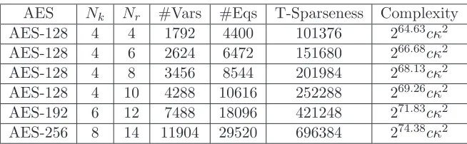
SetNk = 4,6,8, Nr = 4,6,8,10,12,14, and ǫ= 1%. We have the following complexities on
quantum algebraic attack on various AESes. From Table 2, we can see that AES is secure under quantum algebraic attack only if the condition number κ is large.
AES Nk Nr #Vars #Eqs T-Sparseness Complexity
AES-128 4 4 1792 4400 101376 264.63cκ2
AES-128 4 6 2624 6472 151680 266.68cκ2
AES-128 4 8 3456 8544 201984 268.13cκ2
AES-128 4 10 4288 10616 252288 269.26cκ2
AES-192 6 12 7488 18096 421248 271.83cκ2
AES-256 8 14 11904 29520 696384 274.38cκ2
6.2 Quantum algebraic attack against Trivium
Trivium is a synchronous stream cipher designed by Canni´ere and Preneel [7] in 2005 to provide a flexible trade-off between speed and gate count in hardware, and reasonably efficient software implementation, which has been specified as an International Standard under ISO/IEC 29192-3. Trivium can be represented by the following nonlinear feedback shift registers (NFSR) which can also be considered as BMQ [26] F:
A(t+ 93) =A(t+ 24) +C(t+ 45) +C(t) +C(t+ 1)C(t+ 2), 0≤t≤Nr−67;
B(t+ 84) =B(t+ 6) +A(t+ 27) +A(t) +A(t+ 1)A2(t+ 2), 0≤t≤Nr−70; (14) C(t+ 111) =C(t+ 24) +B(t+ 15) +B(t) +B(t+ 1)B(t+ 2), 0≤t≤Nr−67;
z(t) =A(t+ 27) +A(t) +B(t+ 15) +B(t) +C(t+ 45) +C(t), 0≤t≤Nr−1,
whereA, B, Care state variables andzis the output. For an initial stateZ0 = (A(0), . . . , A(92),
B(0), . . . , B(83), C(0), . . . , C(110)) ∈F288
2 , we can generate the key sequencez(0), z(1), . . . , z(Nr
−1) with the above NFSR. Thus, for theNr-round Trivium,F consists of (3Nr−201) quadratic
polynomials of sparseness 5, and Nr linear polynomials of sparseness 7, and with (3Nr + 87)
indeterminates. Thus, T = 5(3Nr−201) + 7Nr = 22Nr−1005.
The algebraic attach on theNr-round Trivium is to solve the BMQ (14), wherez(0), z(1), . . .,
z(Nr−1) are constants. It is generally believed that for Nr>288, (14) has a unique solution.
Proposition 6.2. There is a quantum algorithm to find a solution for the Nr-round Trivium
equation system in time 217.22Nr3.5cκ2log 1/ǫ with probability >1−ǫ, where κ is the condition number of F and c is the complexity constant of the HHL algorithm.
Proof. By Theorem 5.13, the complexity is√2c(log2((3Nr+87)+2(22Nr−1005)−5(4Nr−201))+
((3Nr+87)+(22Nr−1005)−3(4Nr−201)) log2e)((3Nr+87)+(22Nr−1005)−3(4Nr−201)+2r1+
r2)1.5(3(3Nr+87)+9(22Nr−1005)−21(4Nr−201)+12r1+5r2+1)κ2⌈log21/ǫ⌉=
√
2c(log2(27Nr−
918) + (13Nr−315) log2e)(13Nr−315)1.5(123Nr−4562)κ2⌈log21/ǫ⌉ ≤217.22Nr3.5cκ2⌈log21/ǫ⌉.
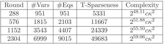
In Table 3, we give the complexities for severalNr assumingǫ= 1%. From Table 3, we can
see that Trivium is secure under quantum algebraic attack only if the condition number κ is large.
Round #Vars #Eqs T-Sparseness Complexity
288 951 951 5331 248.11cκ2
576 1815 2103 11667 251.88cκ2
1152 3543 4407 24339 255.50cκ2
2304 6999 9015 49683 259.06cκ2
Table 3: Complexities of the quantum algebraic attack on Trivium
6.3 Quantum algebraic attack against Keccak
Keccak [5], the winner of SHA-3, is the latest member of the Secure Hash Algorithm family of standards, released by NIST on August 5, 2015. For Keccak-[Nh, b, Nr], we denote Nh, b, and
Nr as the output bit size, the state bit size, and the number of rounds. Let A0(x, y, z) be the
message,Ai(x, y, z) be the state variable after applying theτ function fori-times, andBi(x, y, z)
be the state variable after applying the π function for i-times, where x, y ∈ Z/5Z, z ∈ Z/wZ,
have the following BMQ F [27]:
Bi(3y+x, x, z−r(3y+x, x)) =Ai−1(x, y, z) +
4
X
j=0
Ai−1(x−1, j, z) +
4
X
j=0
Ai−1(x+ 1, j, z−1);
Ai(x, y, z) =Bi(x, y, z) + (1−Bi(x+ 1, y, z))Bi(x+ 2, y, z), forx6= 0 ory6= 0; Ai(0,0, z) =Bi(0,0, z) + (1−Bi(1,0, z))Bi(2,0, z) +RC(z)
fori= 1, . . . , Nr, x, y= 0, . . . ,4,z= 0, . . . , w. In the preimage attack on Keccak, r(3y+x, x)
and RC(z) are known constants, the first Nb of ANr(x, y, z) are the known Hash output, and
Ai(x, y, z) (i < Nr) and Bi(x, y, z) are indeterminates. Thus we have n= 2bNr indeterminates
and r = (2b−1)Nr+Nh Boolean quadratic equations with total sparseness T = 401Nrw+
101Nh/25−101w.
Proposition 6.3. For the BMQ Keccak-[Nh, b, Nr], there is a quantum algorithm to find a
preimage in time√2c(log2(802Nrw+5Nr+77Nh/25)+(401Nrw+3Nr+26Nh/25) log2e)(401Nrw
+3Nr+ 26Nh/25)1.5(3609Nrw+ 21Nr+ 384Nh/25 + 1)κ2⌈log21/ǫ⌉<218.21Nr3.5b3.5cκ2log21/ǫ
with probability >1−ǫ, where κ is the condition number ofF andc is the complexity constant of the HHL algorithm.
Proof. We have n = 2bNr, r = (2b−1)Nr +Nh, and T = 401Nrw+ 101Nh/25−101w. By
Theorem 5.13, the complexity is √2c(log2(2bNr + 2(401Nrw + 101Nh/25−101w) −5((2b−
1)Nr +Nh)) + (2bNr + (401Nrw+ 101Nh/25 −101w) −3((2b −1)Nr +Nh)) log2e)(2bNr +
(401Nrw+ 101Nh/25−101w)−3((2b−1)Nr+Nh))1.5(32bNr+ 9(401Nrw+ 101Nh/25−101w)−
21((2b−1)Nr+Nh) + 1)κ2⌈log21/ǫ⌉ ≤
√
2c(log2(802Nrw+ 5Nr+ 77Nh/25) + (401Nrw+ 3Nr+
26Nh/25) log2e)(401Nrw+ 3Nr+ 26Nh/25)1.5(3609Nrw+ 21Nr+ 384Nh/25 + 1)κ2⌈log21/ǫ⌉ ≤
√
2 log2ec(401Nrw+26Nh/25)2.5(3609Nrw+384Nh/25)κ2⌈log21/ǫ⌉ ≤218.21Nr3.5b3.5cκ2⌈log21/ǫ⌉.
SettingNh = 224,256,384,512, Nr= 24, b= 1600 and ǫ= 1%, the complexities for various
(Nh, b, Nr) are given in Table 4. From Table 4, we can see that Keccak is secure under quantum
algebraic attack only if the condition number κ is large.
Nh b Nr #Vars #Eqs T-Sparseness Complexity
224 1600 24 76800 77000 610377 273.12cκ2
256 1600 24 76800 77032 610506 273.12cκ2
384 1600 24 76800 77160 611023 273.12cκ2
512 1600 24 76800 77288 611540 273.12cκ2
Table 4: Complexities of the quantum preimage attack on Keccak
The best known traditional attacks on Keccak were given in [25] and [17]. In [25], practical collision attacks against the 5-round Keccak-224 and an instance of the 6-round Keccak collision challenge were given. In [17], key recovery attacks were given for 4- to 8-round Keccak.
6.4 Quantum algebraic attack against MPKC
Multivariate Public Key Cryptosystem (MPKC) is one of the candidates for post-quantum cryptography [13]. An MPKC is generally constructed as follows