Demand Patterns Across the Development Spectrum: Estimates for the AIDADS System

(1)

Menzies Building

PO Box 11E, Monash University

Wellington Road

CLAYTON Vic 3800 AUSTRALIA

Telephone:

from overseas:

(03) 9905 2398, (03) 9905 5112 61 3 9905 5112 or 61 3 9905 2398

Fax:

(03) 9905 2426

61 3 9905 2426

e-mail

[email protected]

web site

http://www.monash.edu.au/policy/

D

EMAND

P

ATTERNS

A

CROSS THE

D

EVELOPMENT

S

PECTRUM

:

E

STIMATES

FOR

THE

AIDADS S

YSTEM

by

Maureen T. RIMMER Alan A. POWELL

Industry Commission

and Monash

University

Monash

University

Preliminary Working Paper No. OP–75 October 1992

reissued August 2001

ISSN 1031 9034 ISBN 0 642 10225 2

The Centre of Policy Studies

(CoPS)

is a research centre at Monash University

devoted t o quantit at ive analysis of issues relevant t o Australian economic policy.

C

ENTRE

of

P

OLICY

S

TUDIES

and

the

I

MPACT

(2)

This is a companion paper to

Impact Preliminary Working Paper

No OP-73 in which Rimmer and Powell report on a new

implicitly

directly additive demand system

(AIDADS) which (in Cooper and

McLaren's 1992b terminology) is effectively globally regular. In

OP-73 AIDADS is fitted to a six-commodity disaggregation of a

35-year Australian time series of consumption. Unlike the linear

expenditure system and the Rotterdam model, the new system

allows marginal budget shares to vary as a function of income.

In the current paper we also work at a six-commodity level,

fitting AIDADS to an international cross section of 30 countries in

1975. The data are from the International Comparisons Project

of Kravis, Heston and Summers (1982) and previously were

analyzed by Theil and Clements (1987) using a combination of

additive preferences and Working's (1943) model in differential

form. The present results overcome two potential shortcomings

of the earlier work by replacing Working's model with a more

regular specification of Engel effects and by providing and

estimating an explicit functional form in the

levels

of the

variables.

(3)

iii

Abstract i

1. Introduction 1

2. Brief Description of AIDADS 2

2.1 The new expenditure system 2

2.2 Substitution properties 3

2.3 Engel properties 3

2.4 Estimation of AIDADS 4

3. Empirical Estimates 6

3.1 The Data 6

3.2 Estimating Equation 8

3.3 The ML Estimates 9

3.4 Comparison of the international cross section and the

the Australian time series 16

References 21

Table 3.1.1 Consumption Per Capita for Thirty Countries in

1975 7

Table 3.1.2 The Theil and Clements Ten Commodity Level of

Disaggregation of Final consumption Expenditure 8

Table 3.1.3 The Six-Commodity Disaggregations used for the International Comparisons Data and the Australian

Time-series Data 8

Table 3.3.1 Maximum Likelihood Estimates of AIDADS fitted in

the Levels, 30 Country Cross Section Data for 1975 9

Table 3.3.2 Estimated Engel and Own and Cross-Price Elasticities

for the Low Lowest Income Country 12

Table 3.3.3 Estimated Engel and Own and Cross-Price

Elasticities for the Highest Income Country 13

Table 3.3.4 Estimated Substitution Elasticities from AIDADS

for Richest and Poorest Countries 13

Figure 2.4.1 Flow chart for data/parameter transformations

in computation of the ML estimates 5

Figure 2.4.2 Sample variation in real per capita consumption

in the international comparisons data 6

Figure 3.3.1 Actual and fitted budget shares for international

comparisons data 10

Figure 3.3.2 Estimated marginal budget shares as a function

of affluence 14

Figure 3.3.3 Estimated total expenditure elasticities as function

of affluence 16

Figure 3.4.1 Comparison of behaviour of estimated budget shares in the international cross section and in the

(4)

by

Maureen T. RIMMER and Alan A. POWELL

Industry Commission

and Monash University

Monash University

1. Introduction

Theil and Clements (1987) employed a novel approach to estimate an additive preferences demand system from the international comparisons data constructed by Kravis, Heston and Summers (1982). The motivation for this work sprang partly from the observation that the marginal budget share of food seemed to decline with increasing per capita real consumption. Since marginal budget shares are constant both in the Rotterdam model (see e.g., Theil 1965) and in Stone's (1954) Linear Expenditure System (LES), neither was suitable for Theil and Clements' estimation.

A better Engel specification, and the one used by Theil and Clements, was Working's (1943) formulation in which the budget share of food was written as a linear function in real per capita total expenditure. This is the Engel specification employed in Deaton and Muellbauer's Almost Ideal Demand System (AIDS) (1980).

Theil and Clements did not attempt to make their demand system explicit in the levels of the variables, preferring to work in terms of differentials. Thus the differences in per capita demands for broad commodity aggregates between the thirty or so countries of the international comparisons data were explained by the differences in per capita real total consumption and in relative prices across the cross section. The relatively high level of aggregation (10 commodities) and the need to preserve degrees of freedom led them to impose directly additive preferences. Under the latter specification, it is known (Houthakker 1960) that in any given price/total expenditure locality, the Allen-Uzawa cross partial substitution elasticities are proportional to the product of the Engel elasticities; that is,

(1.1) σ_ij = Ð φ E_i E_j , (φ < 0; i≠j; i, j=1, ..., n)

where the constant of proportionality φ is independent of the particular pair {i, j} of commodities. Whilst φ (closely related to the so-called Frisch (1959) 'parameter') in principle is a function of all prices and total expenditure, Theil and Clements concluded that the dependency was weak in their sample, and treated φ as an absolute constant (which turned out empirically to be about Ð 0.5).

Working's formulation and AIDS share the problem that, under large changes in real incomes, budget shares can stray outside the [0,1] interval. It was such irregular behaviour that led Cooper and McLaren (1987, 1988, 1991, 1992a) to modify the AIDS system to become MAIDS, a system with regular properties over a much wider subset of the price-expenditure space and to propose (1992b) a new class of effectively globally regular (EFG) demand systems. In our current contribution we fit an EFG demand system Ñ one which has proved promising with relatively long (35 years) Australian time

(5)

series data (Rimmer and Powell, 1992) Ñ to the international comparisons data. Our system goes by the acronym AIDADS (an implicitly directly additive demand system)

By effectively global regularity in the current context we mean that AIDADS is regular throughout that part of the price-expenditure space in which the consumer is at least affluent enough to meet subsistence requirements.

The remainder of this paper is structured as follows. In Section 2 the essentials of AIDADS are set out. Results are given in Section 3, which includes a brief description of the data and a comparison with recent time-series work using AIDADS (Rimmer and Powell, 1992).

2. Brief Description of AIDADS

1

2.1 The new expenditure system

Hanoch (1975) defines implicit direct additivity by the utility function:

(2.1.1)

Σ

i=1 n

Ê

U_i(x_i , u) = 1,

where {x₁, x₂, ... , x_n} is the consumption bundle, u is the level of utility, and the U_i are twice-differentiable monotonic functions satisfying appropriate concavity conditions. Using some intuition stemming from Cooper and McLaren's (1992a) and from the LES, we choose the U_i as follows:

(2.1.2) U_i =

[α_iÊ+Êβ_iÊG(u)]

Ê[1Ê+ÊG(u)] ln

(

Êx_iÊÐÊγ_i

ÊAÊeuÊÊ

)

= φi ln

(

Êx_iÊÐÊγ_i

ÊAÊeuÊÊ

)

,

(i = 1, 2, ..., n)

where G(u) is a positive, monotonic, twice-differentiable function, and the lower-case Greek letters and A are parameters, with

(2.1.3) 0 ≤ α_i , β_i ≤ 1;

Σ

i=1 n

Ê_α

i = 1 =

Σ

i=1 n

Ê_β i .

The first-order conditions for minimizing the cost M of obtaining a given level of utility u subject to given prices {p₁_Ê, p₂_{, ..., pn} are (2.1.1) and:}

(2.1.4)

λÊ[

α

_iÊ+Êβ_iÊG(u)]

(

x_iÊÐÊγ_i

)Ê

[1Ê+ÊG(u)] = pi . (i = 1, 2, ..., n)

Hence

(2.1.5) λÐÊ1 p_iÊ(x_i Ð γ_i) = [

α

_i + β_i G(u)] / [1 + G(u)] .

(i = 1, 2, ..., n)

Using the budget identity

(6)

(2.1.6)

Σ

i=1 Ê

p_i x_i = M,

by adding (2.1.5) across i, and using (2.1.3) to solve for λ we obtain:

(2.1.7) λ = (M Ð p′ γ) ,

where p'γ is shorthand for

∑

i=1 n

Ê p_iγ_{i . Back-substituting from (2.1.7) into (2.1.5), after}

rearrangement we obtain

(2.1.8) p_iÊ(x_i Ð γ_i) =

φ

_i (M Ð p′ γ) , (i = 1, 2, ..., n)

where from (2.1.2):

(2.1.9)

φ

_i =

φ

_i (u) =

Ê[

α

_iÊ+Êβ_iÊG(u)]

[1Ê+ÊG(u)Ê]Ê . (i = 1, 2, ..., n)

2.2 Substitution properties

The substitution elasticities associated with implicit direct additivity are:

(2.2.1) σ_{i j} =

(x_iÊÐÊγ_i)Ê(x_jÊÐÊγ_j)Ê

x_iÊx_j

/

(MÊÐÊp′Êγ)Ê

MÊÊ (i≠j, i ,j = 1, 2, ..., n)

= Ð φ* E*_i E*_j where

(2.2.2) φ∗ = Ð (MÊÐÊp′Êγ)Ê MÊÊ

and

(2.2.3) E*_i =

φ

_i / W_i (i = 1, 2, ..., n)

in which W_i is the budget share of i.2

2.3 Engel properties

Not much further progress can be made without specifying a functional form for G. Here we keep the LES interpretation of γ as the subsistence bundle, and require as well that

(2.3.1a) lim

xÊ→Ê

∞

Ê u(x) =

∞

;

(2.3.1b) lim

xÊ→Ê

γ+

Ê u(x) = Ð

∞

;

(7)

(2.3.1c) lim

uÊ→Ê

∞

Ê G(u) =

∞

;

and

(2.3.1d) limÊ

uÊ→Ê

ÐÊ

∞

Ê

Ê G(u) =

0 .

x is the bundle {x₁, x₂, ..., x_n}, and the notation x →

∞

implies that every

x

_i grows without limit, while x →

γ

+ implies that each

x

_{i converges to its corresponding}

γ

_iÊfrom above.) G's monotonicity together with the bounds imposed on it above ensure that

φ

_i behaves logistically, remaining always in the [α_i, β_i] interval. It can be shown that if

α

_i < β_i, the logistic behaviour of

φ

_i implies that the lowest value of i's marginal budget share is

α

_i, occurring when total expenditure is just enough to cover purchase of the subsistence bundle

γ;

theupper asymptote of MBS_iÊ as expenditure grows without limit is β_i. If, on the other hand,

α

_i > β_i, the largest value of i's marginal budget share is

α

_i, occurring at the subsistence expenditure level; its asymptote as expenditure grows indefinitely large and lowest value is β_i.

The Engel elasticities in AIDADS are:

(2.3.2)

ε

_i

=

φ

iÊÊÊM

ÊÊÊp_iÊγ_iÊÊ+ÊÊ

φ

_iÊÊ(MÊÊÊÐÊÊp′Êγ)ÊÊ +

[

∂φ

_i

/∂

Μ

]

ÊΜÊÊ(MÊÊÊÐÊp′Êγ)

φ

_iÊÊ(MÊÊÊÐÊÊp′Êγ)ÊÊ

=

φ

_iÊÊÊM

φ

_iÊÊ(MÊÊÊÐÊÊp′Êγ)ÊÊ +

[

∂φ

_i

/∂

u

]

Ê

[

∂

u

/∂

Μ

]

ÊΜÊÊ(MÊÊÊÐÊÊp′Êγ)

φ

_iÊÊ(MÊÊÊÐÊÊp′Êγ)ÊÊ .

(i = 1, 2, ..., n)

Further progress cannot be made without specifying a functional form for G. The simplest G(¥) satisfying (2.3.1c&d) is:

(2.3.3) G(u) =

e

u .

In this case

(2.3.4)

∂φ

_i

/∂

u = (_β_i Ð

φ

_{i ) e}u /(1 + eu) . (i = 1, 2, ..., n)

An expression for

∂

u

/∂

Μ is given in Rimmer and Powell (1992) .

2.4 Estimation of AIDADS

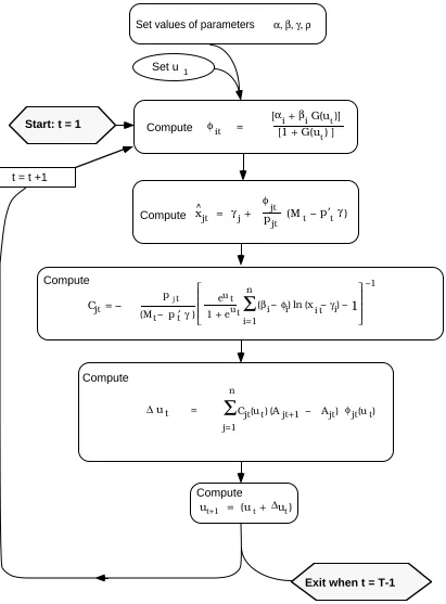
Because the expenditure system (2.1.9) depends via φ_i on the implicitly defined and unobservable variable u, estimation of AIDADS requires an initial level u₁ of u to be treated as a parameter. When moving from an initial data point (here, read 'country') with exogenous variable coordinates {M; p_1Ê, p₂_{, ..., pn}}₁ to the next data point with exogenous variable coordinates {M; p₁, p₂_{, ..., pn} 2, we need to be able to show how the} change in utility level ∆u₁ depends on the parameters (which are common across countries) of the utility function and on the differences between total per capita expenditure and prices in the two. In Rimmer and Powell (1992) it is shown that this can be achieved using the scheme shown in Figure 2.4.1. Note that in this figure x^_i_t is short-hand for the solution of (2.1.8) in terms of xÊ_i_t, while the A_jt are:

(8)

Compute Compute

C_jt = Ð

p_j_t (MÊ ÐÊ p_t _t′ γ)_



  

eu 1Ê+Êe

Σ

i=1 n

βÊÐ φ)ÊlnÊ(x _i)ÊÐÊ₁

Ð1 t

t

 

 

u Ê( i i iÊÐÊt γ

φ_it = [α_[1Ê+ÊG(uiÊ+ÊβiÊG(ut)]

t)Ê]Ê

Compute

t = t +1

Set u ₁

Set values of parameters α, β, γ, ρ

x ^

jt = γj +

φ

jtÊ

p_jt (Mt Ð p′t γ)

Compute Ê

Compute

u_t+1 = (u_t + ∆u_t) ∆u_t =

Σ

j=1 n

C_jt(u )Ê(A_t _jt+1ÊÊÐÊÊÊÊA )ÊÊ_jt φ_jt(u )_t Ê ÊÊ Ê

Ê

Exit when t = T-1 Start: t = 1

Ê Ê

[after Rimmer and Powell (1992)]

(9)

To keep the differences between sample points small (and therefore amenable to the use of differential analysis as in Figure 2.4.1), we followed Theil and Clements (1987) and arranged the cross-section of countries in a series according to increasing order of real per capita total expenditure. The plot of rank against real (international dollar) expenditure per head is shown in Figure 2.4.2 (the actual data are shown below in Table 3.1.1).

natural log of real per capita consumption

0 1 2 3 4 5 6 7 8 9

1 3 5 7 9 11 13 15 17 19 21 23 25 27 29 rank acccording to real per capita consumption

Figure 2.4.2 Sample variation in real per capita consumption in the international comparisons data

3. Empirical Estimates

3.1 The Data

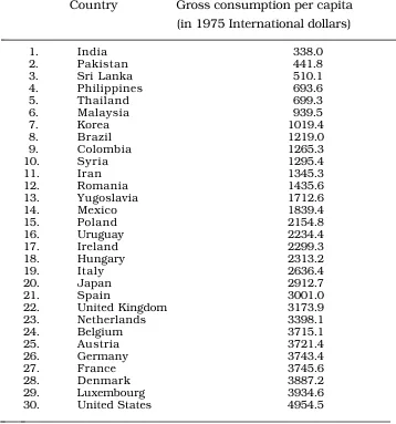
The estimation of AIDADS requires data on nominal total expenditure as well as commodity prices. For each of thirty countries3_{from the International Comparison}

Project listed in Table 3.1.1, Theil and Clements extracted data on real total consumption expenditure and real expenditure by commodity in 1975 expressed in Òinternational dollarsÓ4_{, Q}

t being real total consumption expenditure in country t and xit being real consumption expenditure on commodity i in country t. In addition they used data on the budget shares w_itÊ of commodity i in country t. The commodity data were at the ten commodity level of disaggregation as listed in Table 3.1.2.

3_{There were thirty-four countries in the Kravis, Heston and Summers study. Of these four}

countries were rejected by Theil and Clements. Kenya, Zambia and Malawi were omitted as outliers and because Kravis et al. regarded the data for these countries as beset with numerous problems. The fourth country, Jamaica, was omitted because it had an exceptionally large budget share devoted to Òother Ò expenditure.

4_{International prices are used to value the category quantities in each country under study in}

(10)

Consumption Per Capita For Thirty Countries in 1975 (from the International Comparisons Project)

Country Gross consumption per capita (in 1975 International dollars)

1. India 338.0

2. Pakistan 441.8

3. Sri Lanka 510.1

4. Philippines 693.6

5. Thailand 699.3

6. Malaysia 939.5

7. Korea 1019.4

8. Brazil 1219.0

9. Colombia 1265.3

10. Syria 1295.4

11. Iran 1345.3

12. Romania 1435.6

13. Yugoslavia 1712.6

14. Mexico 1839.4

15. Poland 2154.8

16. Uruguay 2234.4

17. Ireland 2299.3

18. Hungary 2313.2

19. Italy 2636.4

20. Japan 2912.7

21. Spain 3001.0

22. United Kingdom 3173.9

23. Netherlands 3398.1

24. Belgium 3715.1

25. Austria 3721.4

26. Germany 3743.4

27. France 3745.6

28. Denmark 3887.2

29. Luxembourg 3934.6

30. United States 4954.5

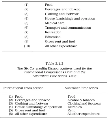
For comparison purposes with the AIDADS estimates obtained by Rimmer and Powell (1992) from Australian time series, this international data set of Theil and Clements was aggregated to six commodity groups as shown in Table 3.1.3. They are

very roughly comparable to the commodity categories in the Australian study.

Relative price data π_it (with the price of food the numeraire) were obtained for each of the six commodity groups in Table 3.1.3 in each country as the ratios

w_itÊx_1tÊ

Êw_1tÊx_itÊÊ of each budget share otherthan for Food to that of Food multiplied by the

(11)

Table 3.1.2

The Theil and Clements Ten Commodity Level of Disaggregation of Final Consumption Expenditure

(1) Food

(2) Beverages and tobacco (3) Clothing and footwear

(4) House furnishings and operation (5) Medical care

(6) Transport and communication (7) Recreation

(8) Education

(9) Gross rent and fuel (10) All other expenditure

Table 3.1.3

The Six-Commodity Disaggregations used for the International Comparisons Data and the

Australian Time-series Data

International cross section Australian time series

(1) Food Food

(2) Beverages and tobacco Alcohol & tobacco (3) Clothing and footwear Clothing and footwear (4) House furnishings & operation Durables

(5) Gross rent and fuel Rent

(6) All other expenditure All other expenditure

3.2 Estimating Equation

The expenditure system (2.1.8) was estimated in the form:

(3.2.1) W_it = φ_it +









p_itγ_iÊÐÊφ_iÊp′_tÊγ

Μ_t + vÊ_{it ,} ( i = 1, 2, ..., n)

where W_it is the budget share of the ith commodity in the tth country , and vÊ_it is a zero-mean random error, assumed normally distributed and independent of v_it±Ê _τ (for all

integral τ≠ 0). Full information maximum likelihood estimates were computed with the v a r i a n c e - c o v a r i a n c e m a t r i x o f t h e vÊ_{i t s c o n s t r a i n e d ˆ l a} Selvanathan (1991).5_{Because the variables {}φ

(12)

1 2 tÐ1

before u_t can be evaluated (see Figure 2.4.1), flexible software is needed. We found

GAUSS 386 on a 486 personal computer up to the task.

3.3 The ML Estimates

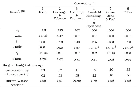
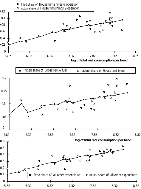
We fitted AIDADS in the levels using the Theil and Clements cross section data described above. The results of that estimation appear in Table 3.3.1. The fitted and actual budget shares are plotted in Figure 3.3.1.

Table 3.3.1

Maximum Likelihood Estimates of AIDADS fitted in the Levels, 30 Country Cross Section Data for 1975

Commodity i Item(a)Ê(b) 1 Food 2 Beverage & Tobacco 3 Clothing & Footwear 4 Household Furnishing s & Operations 5 Gross Rent & Fuel 6 Other α_i t ratio .693 18.15 .125 4.47 .182 6.01 .000 0.01 .000 0.00 .000 0.01 β_i t ratio .000 0.00 .023 0.29 .049 1.57 .125

11×103

.183

64×103

.620

24×103 γ_i t ratio 112.33 7.59 0.91 1.82 0.07 0.71 0.02 0.31 13.13 2.05 0.08 0.64

Marginal budget shares ψ_it:

poorest country richest country .33 .02 .07 .03 .11 .05 .07 .12 .10 .18 .33 .60 Durbin-Watson statistic

1.96 1.97 01.69 1.79 1.55 1.95

utility level for the poorest country, u1 = Ð0.869: utility level in for the richest country, u_T = +1.290.

t value for uT = 16.44.

(13)

0 0.1 0.2 0.3 0.4 0.5 0.6 0.7

5.82 6.32 6.82 7.32 7.82 8.32 8.82

fitted share of

actual share of

Food

0 0.02 0.04 0.06 0.08 0.1 0.12

5.82 6.32 6.82 7.32 7.82 8.32 8.82

log of total real consumption per head

0 0.02 0.04 0.06 0.08 0.1 0.12 0.14 0.16

5.82 6.32 6.82 7.32 7.82 8.32 8.82

fitted share of Clothing & footwear

actual share of Clothing & footwear

fitted share of Beverages & tobacco

actual share of Beverages & tobacco

Food

(14)

0 0.02 0.04 0.06 0.08 0.1 0.12

5.82 6.32 6.82 7.32 7.82 8.32 8.82

log of total real consumption per head fitted share of

House furnishings & operation

actual share of

House furnishings & operation

fitted share of All other expenditure

actual share of All other expenditure

0 0.1 0.2 0.3 0.4 0.5 0.6

5.82 6.32 6.82 7.32 7.82 8.32 8.82

fitted share of Gross rent & fuel

actual share of Gross rent & fuel

0 0.05

0.1

0.15 0.2

5.82 6.32 6.82 7.32 7.82 8.32 8.82

(15)

half of the countries, a downward trend in budget share with increasing affluence can be detected.

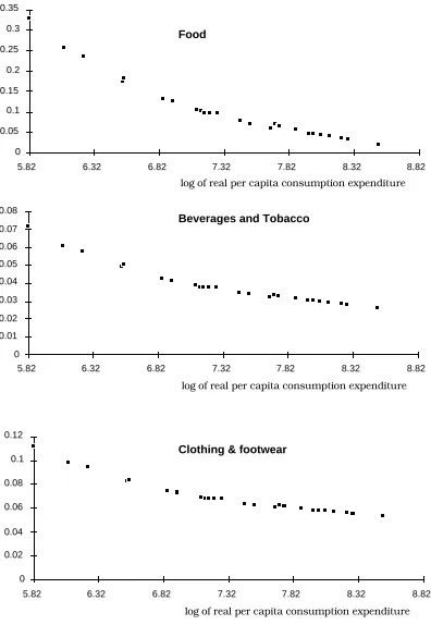
Corner solutions were obtained for the α_i value for House furnishings and Operation, Gross rent and Fuel, and All other expenditure, while effectively zero subsistence quantities were found for all commodities except Food and All other expenditure. In keeping with the findings of Theil and Clements (1987) and the Adams, Chung and Powell (1988), the estimates show a strongly decreasing marginal budget share (MBS) for Food, from 0.33 to 0.02, whereas the AIDADS estimates for time series Australian data show an almost constant marginal budget shares for Food of around 0.07. The difference between the two AIDADS results can be explained substantially in terms of the span of real income across the samples. Figure 3.3.2 shows the MBSÕs for the countries in the cross section study. From Figure 3.3.2 it can be seen that for the majority of the countries very little change in the MBS for Food was observed and for countries within the time-series income range of Australia6_{, values ranged between 0.08}

and 0.03 .

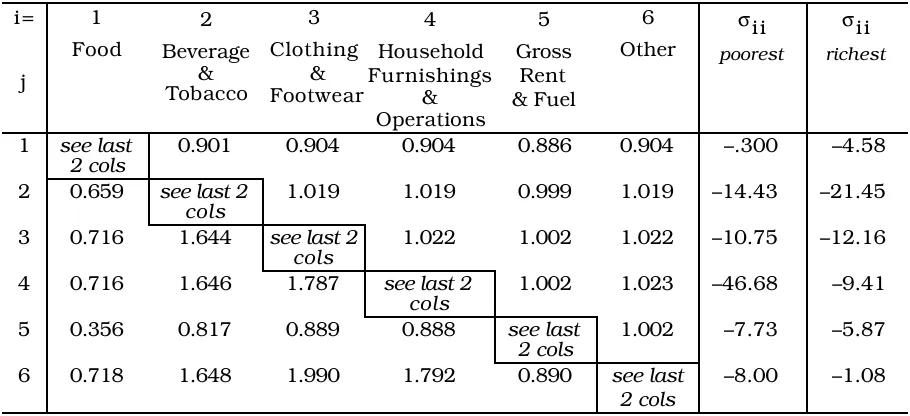
Own and cross price elasticities of demand and Engel elasticities are given in Tables 3.3.2 and 3.3.3 respectively for the least affluent and most affluent countries in the sample. At constant prices it can be shown that the Engel elasticities for AIDADS tend to unity as expenditure grows without limit. However this movement towards unity need not be monotonic. With substantial price variation across countries, as is occurring in this cross section study, this pattern of movement to unity in Engel elasticities can be further obscured. The Engel elasticities are graphed in Figure 3.3.3. Movement of the Engel elasticity away from unity with increasing affluence is particularly evident for the necessity Food. As for the AIDADS estimation on Australian time series data, several of the cross price elasticities are positive indicating gross substitutability rather than gross complementarity. The estimated elasticities of substitution are shown for the richest and poorest countries in Table 3.3.4.

Table 3.3.2

Estimated Engel and Own and Cross-Price Elasticities for the Low Lowest Income Country*

Price which changes, j

Commodity

1 Food

2 Alcohol

& Tobacco

3 Clothing

& Footwear

4 Durables

5 Rent

6 Other

Engel Elasticity

ε_i

1 Ð0.530 _0.010 _0.1853 _0.005 _Ð0.008 _0.024 _.485

2 Ð 0.400 Ð0.902 0.032 0.008 Ð0.026 0.041 1.246 3 Ð0.473 0.013 Ð0.966 0.008 Ð0.032 0.039 1.411 4 Ð1.678 Ð0.088 Ð0.111 Ð1.0265 Ð0.139 Ð0.142 3.184 5 Ð0.833 Ð0.044 Ð0.055 Ð0.014 Ð0.564 Ð0.010 1.581 6 Ð1.681 Ð0.089 Ð0.111 Ð0.029 Ð0.139 Ð1.141 3.190

* Based on parameter estimates shown in Table 3.3.1.

6 _{AustraliaÕs per capita income range across the sample period 1954-55 through 1988-89 is}

(16)

Estimated Engel and Own and Cross-Price Elasticities for the Highest Income Country

Price which changes, j

Commodity 1 Food 2 Alcohol & Tobacco 3 Clothing & Footwear 4 Durables 5 Rent 6 Other Engel Elasticity ε_i

1 Ð0.773 0.034 0.059 0.075 0.1096 0.371 .124 2 0.051 Ð0.078 0.032 0.041 0.058 0.202 .596 3 0.034 0.014 Ð0.975 0.031 0.043 0.154 .698 4 Ð0.054 Ð0.011 Ð0.018 Ð1.023 Ð0.037 Ð0.115 1.264 5 Ð0.058 Ð0.011 Ð0.018 Ð0.023 Ð1.017 Ð0.113 1.240 6 Ð0.059 Ð0.011 Ð0.018 Ð0.023 Ð0.037 Ð1.115 1.264

* Based on parameter estimates shown in Table 3.3.1.

Table 3.3.4

Estimated Substitution Elasticities from AIDADS for Richest and Poorest Countries*

i = j 1 Food 2 Beverage & Tobacco 3 Clothing & Footwear 4 Household Furnishings & Operations 5 Gross Rent & Fuel 6 Other

σ_{i i}

poorest

σ_{i i}

richest

1 see last 2 cols

0.901 0.904 0.904 0.886 0.904 Ð.300 Ð4.58

2 0.659 see last 2 cols

1.019 1.019 0.999 1.019 Ð14.43 Ð21.45

3 0.716 1.644 see last 2 cols

1.022 1.002 1.022 Ð10.75 Ð12.16

4 0.716 1.646 1.787 see last 2 cols

1.002 1.023 Ð46.68 Ð9.41

5 0.356 0.817 0.889 0.888 see last 2 cols

1.002 Ð7.73 Ð5.87

6 0.718 1.648 1.990 1.792 0.890 see last 2 cols

Ð8.00 Ð1.08

(17)

0 0.05 0.1 0.15 0.2 0.25 0.3 0.35

5.82 6.32 6.82 7.32 7.82 8.32 8.82

0 0.01 0.02 0.03 0.04 0.05 0.06 0.07 0.08

5.82 6.32 6.82 7.32 7.82 8.32 8.82

0 0.02 0.04 0.06 0.08 0.1 0.12

5.82 6.32 6.82 7.32 7.82 8.32 8.82

Food

Beverages and Tobacco

Clothing & footwear

log of real per capita consumption expenditure

(18)

0 0.02 0.04 0.06 0.08 0.1 0.12

5.82 6.32 6.82 7.32 7.82 8.32 8.82

0 0.02 0.04 0.06 0.08 0.1 0.12 0.14 0.16 0.18

5.82 6.32 6.82 7.32 7.82 8.32 8.82

0 0.1 0.2 0.3 0.4 0.5 0.6 0.7

5.82 6.32 6.82 7.32 7.82 8.32 8.82

House furnishings and operation

Gross rent and fuel

All other expenditure

(19)

0 0.05

0.1 0.15

0.2 0.25

0.3 0.35

0.4 0.45

0.5

5.82 6.23 6.55 6.93 7.14 7.20 7.45 7.68 7.74 7.88 8.01 8.13 8.22 8.23 8.28

0 0.2 0.4 0.6 0.8 1 1.2 1.4

0 0.2 0.4 0.6 0.8 1 1.2 1.4 1.6

5.82 6.23 6.55 6.93 7.14 7.20 7.45 7.68 7.74 7.88 8.01 8.13 8.22 8.23 8.28

Food

Beverages and tobacco

Clothing and footwear

log of total real consumption per head log of total real consumption per head

log of total real consumption per head

(20)

0 0.5 1 1.5 2 2.5 3

5.82 6.23 6.55 6.93 7.14 7.20 7.45 7.68 7.74 7.88 8.01 8.13 8.22 8.23 8.28

0 0.2 0.4 0.6 0.8 1 1.2 1.4 1.6 1.8 2

0 0.5 1 1.5 2 2.5 3 3.5

House furnishings & operation

5.82 6.23 6.55 6.93 7.14 7.20 7.45 7.68 7.74 7.88 8.01 8.13 8.22 8.23 8.28

(21)

3.4 Comparison of the international cross section and the Australian time series

Strict comparison between the international cross section results and the time-series results of Rimmer and Powell (1992) is not possible because of different definitions of the broad commodity groups (see Table 3.1.3). However, in order to make a rough comparison, price variations across countries and over time must be removed and a common measure of total expenditure adopted. Two separate computations were carried out in order to produce synthetic 'samples' in which the relative price variation had been removed: one for the cross section study, and one for the time series study.

For the cross section, prices for the six commodities under study were fixed at their geometric mean (across countries) and for each country nominal total expenditure was adjusted so that the country was Ôjust as well offÕ7_{as in the original sample used in}

the AIDADS estimation above. In the case of the Australian time-series, the relative prices of the commodities were fixed at the same values as in the synthetic cross section and total nominal consumption expenditure was adjusted in each sample year to leave each time-series value of per capita utility constant after the price change.

From the two synthetic samples, budget shares of commodities were obtained as a function of real total consumption expenditure Ñ valued in 1975 international dollars in the case of the cross section study, and in 1984-85 Australian dollars for the time series. Real total consumption expenditure for Australia in 1975 in international dollars was available in Summers and Heston (1984). This figure was used to scale the other years of the Australian study to the 1975 international dollar base.

The budget shares from the cross-section and the time-series synthetic samples are plotted in Figure 3.4.1. In the case of Food, the Australian sample has been extrapolated backward to examine whether at very low income levels the time-series estimate of Food's budget share would be substantially different from the value implied by the cross sectional fit. Although the time-series and the cross section show substantial differences in curvature, there is very little difference in Food's budget share at very low and at very high incomes.

However, the difference in shape significantly colours perceptions of the rate of decline of Food's marginal budget share as a function of real per capita expenditure. Over the thirty or so years of the Australian sample, there was a decline in this MBS from 0.080 to 0.076 (Rimmer and Powell, Table 5.2), whereas the poorest and the richest country's MBSs for Food are estimated at 0.33 and 0.02 respectively. The gap between contemporary Australian behaviour (MBSFOOD = 0.076) and American (MBSFOOD = 0.02) is

probably a consequence of the inclusion of the service component of restaurant meals in the Australian (but not the American) data.8

7_{In the AIDADS estimation each countryÕs utility is estimated: the first countryÕs utility level}

is an estimated parameter of the system and the utility levels for the remaining countries are obtained using the scheme set out in Figure 2.4.1.

(22)

0 0.1 0.2 0.3 0.4 0.5

0 1000 2000 3000 4000 5000

Food

total per capita consumption expenditure (international dollars)

0 0.05

0.1 0.15 0.2 0.25 0.3 0.35 0.4 0.45

0 1000 2000 3000 4000 5000

0 0.05

0.1 0.15

0.2 0.25

0.3 0.35

0.4 0.45

0 1000 2000 3000 4000 5000

Beverages and tobacco

international cross section

Australian time series 1954-1989

international cross section

Australian time series 1954-1989

Clothing and footwear

international cross section

Australian time series 1954-1989

backward extrapolation

of Australian time-series data

(23)

0 0.05

0.1 0.15 0.2 0.25 0.3 0.35 0.4 0.45

0 1000 2000 3000 4000 5000

international cross section

Australian time series 1954-1989

international cross section

Australian time series 1954-1989

international cross section

Australian time series 1954-1989

0 0.05

0.1 0.15 0.2 0.25 0.3 0.35 0.4 0.45 0.5

0 1000 2000 3000 4000 5000

0 0.05

0.1 0.15 0.2 0.25 0.3 0.35 0.4 0.45

0 1000 2000 3000 4000 5000

total per capita consumption expenditure (international dollars) House furnishings and operation

(24)

Adams, Philip D., Ching-Fan Chung and Alan A. Powell (1988) "Australian Estimates of Working's Model under Additive Preferences: Revised Estimates of a Consumer Demand System for Use by CGE Modellers and Other Applied Economists", Impact Project Working Paper No. O-61, Industries Assistance Commission, Melbourne, August.

Alaouze, Chris M. (1977) "Estimates of the Elasticity of Substitution between Imported and Domestically Produced Goods Classified at the Input-Output Level of Aggregation", Impact Project Working Paper No. O-13, Industries Assistance Commission, Melbourne, October.

Barten, Anton (1968) "Estimating Demand Equations ", Econometrica, Vol. 36, No. 2 (April), pp. 213-51.

Cooper, R.J. and K.R. McLaren (1987) "Regular Alternatives to the Almost Ideal Demand System", Monash University, Department of Econometrics and Operations Research, second draft, mimeo (December).

Cooper, R.J. and K.R. McLaren (1988). "Regular Alternatives to the Almost Ideal Demand System". Paper presented to the Sixth Analytic Economics Workshop, Australian Graduate School of Management. Monash University, Department of Econometrics and Operations Research, third draft, mimeo (February). A further revision available in Monash University Department of Econometrics Working Paper No 12/88 (September). Cooper R.J. and K.R. McLaren (1991) "An Empirically Oriented Demand System with

Improved Regularity Properties", Monash University Department of Econometrics Working Paper No 8/91.

Cooper, R.J. and K.R. McLaren (1992a) "An Empirically Oriented Demand System with Improved Regularity Properties", Canadian Journal of Economics, Vol.25, pp. 652-67. Cooper, R.J. and K.R. McLaren (1992b) "A System of Demand Equations Satisfying

Effectively Global Regularity Conditions", Department of Econometrics, Monash University, mimeo (July).

Deaton, Angus and John Muellbauer (1980) "An Almost Ideal Demand System", American Economic Review, Vol. 70, pp. 312-26.

Frisch, Ragnar (1959) "A Complete Scheme for Computing All Direct and Cross Elasticities in a Model with Many Sectors", Econometrica, Vol. 27, pp. 177-196.

Hanoch, Giora (1975) "Production or Demand Models with Direct or Indirect Implicit Additivity", Econometrica, Vol. 43, No. 3 (May), pp. 395-419.

Houthakker, H.S. (1960) "Additive Preferences", Econometrica, Vol. 28, No. 2 (April 1960), pp. 244-257.

Kravis, I.B., A.W. Heston and R. Summers (1982) World Product and Income: International Comparisons of Real Gross Product (Baltimore: Johns Hopkins University Press). McLaren, K. R. (1991) "The Use of Adjustment Cost Investment Models in Intertemporal

Computable General Equilibrium Models", Impact Project Preliminary Working Paper No. IP-48, University of Melbourne, Melbourne, March.

Pearson, K. R. (1991) "Solving Nonlinear Economic Models Accurately via a Linear Representation", Impact Project Preliminary Working Paper No. IP-53, University of Melbourne, Melbourne, July.

Selvanathan, Saroja (1991) "The Reliability of ML Estimators of Systems of Demand Equations: Evidence from OECD Countries", Review of Economics and Statistics, Vol. 73, pp. 346-53.

Rimmer, Maureen T. and Alan A. Powell (1992) "An Implicitly Directly Additive Demand System: Estimates for Australia", Impact Project Preliminary Working Paper No. OP-73, Monash University, Clayton, Vic., Australia, October.

Stone, Richard (1954) "Linear Expenditure System and Demand Analysis: An Application to the British Pattern of Demand", Economic Journal, Vol. 64, No. 255 (September 1954), pp. 511-32.

Summers, R. and A. Heston (1984) "Improved International Comparisons of Real Product and its Composition: 1950-1980", Review of Income and Wealth, Vol.30, pp.207-68.

Theil, Henri (1965) "The Information Approach to Demand Analysis", Econometrica, Vol. 33, No. 1 (January), pp. 67-87.

Theil, Henri (1967) Economics and Information Theory (Amsterdam: North-Holland). Theil, Henri, and Kenneth W. Clements (1987) Applied Demand Analysis (Cambridge, Mass:

Ballinger).