Error
evolution
in
multi-step
ahead
streamflow
forecasting
for
the
operation
of
hydropower
reservoirs
Georgia Papacharalampous*, Hristos Tyralis, and Demetris Koutsoyiannis
Department of Water Resources and Environmental Engineering, School of Civil Engineering, National Technical University of Athens, Iroon Polytechniou 5, 157 80 Zografou, Greece
* Corresponding author, [email protected]
Abstract: Multi-step ahead streamflow forecasting is of practical interest for the operation of hydropower reservoirs. We provide generalized results on the error evolution in multi-step ahead forecasting by conducting several large-scale experiments based on simulations. We also present a multiple-case study using monthly time series of streamflow. Our findings suggest that some forecasting methods are more useful than others. However, the errors computed at each time step of a forecast horizon within a specific case study strongly depend on the case examined and can be either small or large, regardless of the forecasting method used and the time step of interest.
KeyWords: hydropower; errors; multi-step ahead forecasting; recursive method; simulations
1.
Introduction
The available methodologies for time series forecasting regarding the forecasting horizon can be classified as one- and multi-step ahead forecasting. There are five strategies for multi-step ahead forecasting, namely the recursive, direct, DirRec, MIMO and DIRMO (Bontempi et al. 2013, Taieb et al. 2012). Despite its far more challenging nature in comparison to one-step ahead forecasting, multi-step ahead forecasting is a common practice in hydrology (e.g. Papacharalampous et al. (2017b), Valipour et al. (2013)) and beyond. Moreover, it is of particular importance for the operation of hydropower reservoirs (e.g. Ballini et al. (2001), Cheng et al. (2008), Coulibaly et al. (2000), Luna et al. (2009)) and, by extension, for the energy industry, especially if we consider that hydropower is a form of energy both reliable and sustainable (Koutsoyiannis 2011).
Herein, we conduct several large-scale computational experiments based on simulations to provide generalized results on the error evolution in multi-step ahead forecasting. We additionally conduct a multiple-case study using monthly time series of streamflow to highlight important facts, which exhibit greater interest when presented using real-world data. Our aim
2
is to create a representative image of the underlying phenomena and, thus, we compare an adequate number of forecasting methods on a large number of time series. The latter are simulated according to a linear model of stationary stochastic processes, which is widely used for the modelling of hydrological processes.
2.
Methodological
framework
2.1
Time series
We simulate time series according to the ARFIMA(p,d,q) model, where ARFIMA stands for Autoregressive Fractionally Integrated Moving Average. Although this specific modelling is accompanied by certain problems (Koutsoyiannis 2016), it is considered rather satisfying for the present study and has been widely applied in the literature (e.g. Montanari et al. (1997)). We use the fracdiff.sim algorithm of the fracdiff R package (Fraley et al. 2012) to simulate time series of the types stated in Table 1.
Table 1. Types of time series simulated in the present study.
Time series type Simulated process Time series length
1a ARFIMA(0,0.30,0) 150
1b 350
2a ARFIMA(1,0.30,0) 150
2b 350
3a ARFIMA(0,0.30,1) 150
3b 350
For the real-world case study we use 92 mean monthly time series of streamflow, which originate from catchments in Australia and are extracted from a larger data set (Peel et al. 2000). We use the deseasonalized time series for the application of the forecasting methods. To describe the long-term persistence of the deseasonalized time series we estimate their Hurst parameter H using the mleHK algorithm of the HKprocess R package (Tyralis 2016), which implements the maximum likelihood method (Tyralis and Koutsoyiannis 2011). The parameter H ranges in the interval (0,1) and values > 0.5 indicate long-range dependence of the Hurst - Kolmogorov stochastic process, which is widely used for the modelling of geophysical processes instead of the ARFIMA(0,d,0) model. The estimated values range between 0.56 and 0.99 with a mean value of 0.78.
2.2
Forecasting methods
3
package rminer (Cortez 2010, 2016), as also several built-in R algorithms (R Core Team 2017). The R package rminer uses the nnet algorithm of the nnet R package (Venables and Ripley 2002) the randomForest algorithm of the randomForest R package (Liaw and Wiener 2002) and the ksvm algorithm of the kernlab R package (Karatzoglou et al. 2004) for the application of the neural networks, random forests and support vector machines respectively. The source code for the implementation of the forecasting methods, as well as generalized information about their performance when applied to linear stochastic processes, can be found in Papacharalampous et al. (2017a).
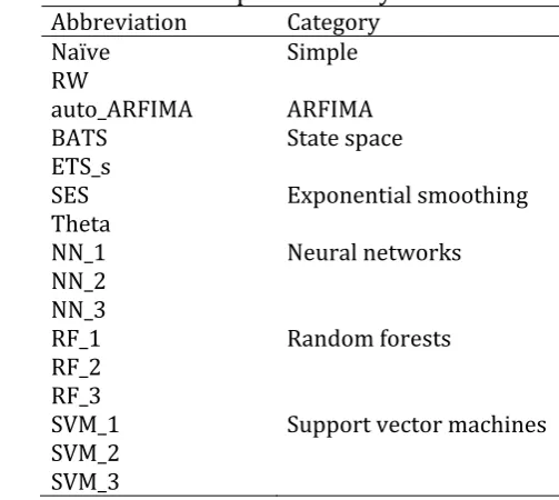
Table 2. Forecasting methods used in the present study.
Abbreviation Category
Naïve Simple
RW
auto_ARFIMA ARFIMA
BATS State space
ETS_s
SES Exponential smoothing
Theta
NN_1 Neural networks
NN_2 NN_3
RF_1 Random forests
RF_2 RF_3
SVM_1 Support vector machines
SVM_2 SVM_3
2.3
Methodology outline
4
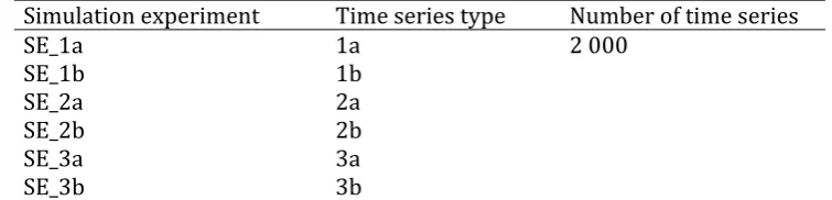
Table 3. Simulation experiments of the present study. The time series types are presented in Table 1.
Simulation experiment Time series type Number of time series
SE_1a 1a 2 000
SE_1b 1b
SE_2a 2a
SE_2b 2b
SE_3a 3a
SE_3b 3b
Within the simulation experiments we carry out a statistical analysis on the formed data sets and we present the results accordingly. As regards the real-world time series, the fitting set is used after deseasonalization, which is performed using a multiplicative model of time series decomposition, while the seasonality is subsequently added to the predicted time series. This specific practice is suggested for the improvement of the forecast quality (Taieb et al. 2012). We present the results of the multiple-case study in a qualitative form to facilitate the detection of systematic patterns.
3.
Results
and
discussion
3.1
Simulation experiments
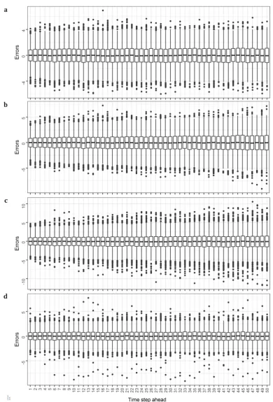
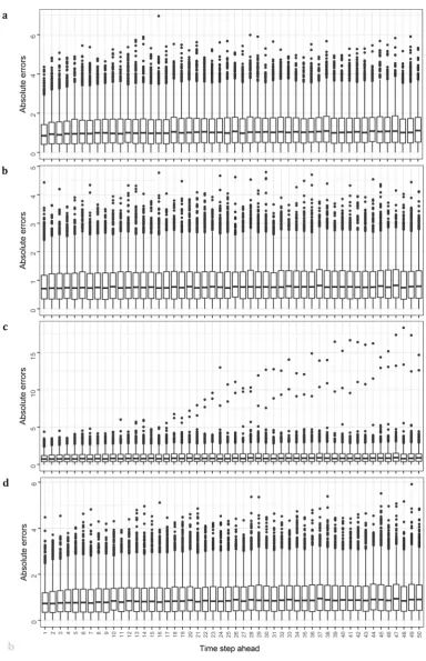
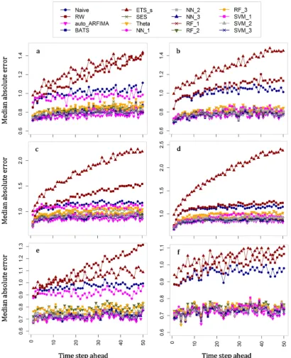
In Section 3.1 we present a representative part of the results of the simulation experiments to support our generalized findings. In more detail, in Figure 1 and Figure 2 we present the errors and the absolute errors computed at each time step of the forecast horizon within the simulation experiment SE_1a for several of the forecasting methods respectively, while in Figure 3 we present the median absolute errors within each of the forecasting experiments for the total of the forecasting methods.
5
Particularly noteworthy is the fact that forecasting methods sharing a quite similar performance within the experiments of Papacharalampous et al. (2017a) are somehow differentiated through the experiments of the present study, e.g. auto_ARFIMA and BATS, Naïve and RW.
6
7
Figure 3. Median absolute errors computed at each time step of the forecast horizon within the simulation experiments (a) SE_1a, (b) SE_1b, (c) SE_2a, (d) SE_2b, (e) SE_3a and (f) SE_3b.
8
general higher on the ARFIMA(1,0.30,0) processes and lower on the ARFIMA(0,0.30,1) processes than they are on the ARFIMA(0,0.30,0) processes, while they are also lower for the fitting set of 300 values than they are for the fitting set of 100 values.
3.2
Multiple-case study
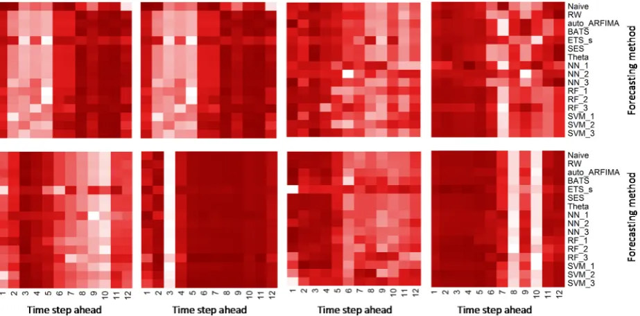
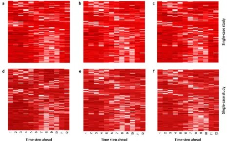
In Section 3.2 we present a part of the results of the multiple-case study. In more detail, in Figure 4 we present eight heatmaps, each corresponding to a specific single-case study, and in Figure 5 we present six heatmaps, each corresponding to the cross-case synthesis of the results of the 92 single-case studies when using a specific forecasting method. These heatmaps can facilitate the comparison of the absolute errors within and across the various single-case studies in a representative manner.
Figure 4. Heatmaps for the comparison of the absolute errors computed at each time step of the forecast horizon within several single-case studies. The values are scaled in the row direction and the darker the colour the better the forecasts.
9
Figure 5. Heatmaps for the comparison of the absolute errors computed at each time step of the forecast horizon across the 92 individual cases when using the (a) Naïve, (b) auto_ARFIMA, (c) BATS, (d) ETS_s, (e) RF_1 and (f) SVM_2 forecasting methods. The values are scaled in the row direction and the darker the colour the better the forecasts.
4.
Conclusions
We deliver generalized results on the error evolution in multi-step ahead forecasting using the recursive technique by comparing the performance of 16 forecasting methods. The present study is an expansion of Papacharalampous et al. (2017a), as it provides complementary information about the forecasting methods also implemented in the latter. Our findings indicate that the error evolution can differ to a great extent from the one forecasting method to the other. This specific information can be used to decide on a forecasting method, since some forecasting methods have been proven more useful than others.
10
References
Ballini, R., Soares, S., and Andrade, M.G., 2001. Multi-step-ahead monthly streamflow forecasting by a neurofuzzy network model. IFSA World Congress and 20th NAFIPS International Conference, 992-997. doi:10.1109/NAFIPS.2001.944740
Bontempi, G., Taieb, S.B., and Le Borgne, Y.A., 2013. Machine learning strategies for time series forecasting. In: M.A. Aufaure, E. Zimányi, eds. Business Intelligence. Springer Berlin Heidelberg, pp 62-77. doi:10.1007/978-3-642-36318-4_3
Cheng, C.T., Xie, J.X., Chau, K.W., and Layeghifard, M., 2008. A new indirect multi-step-ahead prediction model for a long-term hydrologic prediction. Journal of Hydrology, 361 (1-2), 118-130. doi:10.1016/j.jhydrol.2008.07.040
Cortez, P., 2010. Data Mining with Neural Networks and Support Vector Machines Using the R/rminer Tool. In: P. Perner, eds. Advances in Data Mining. Applications and Theoretical Aspects. Springer Berlin Heidelberg, pp 572-583. doi:10.1007/978-3-642-14400-4_44 Cortez, P., 2016. rminer: Data Mining Classification and Regression Methods. R package version
1.4.2. https://cran.r-project.org/web/packages/rminer/index.html
Coulibaly, P., Anctil, F., and Bobee, B., 2000. Daily reservoir inflow forecasting using artificial neural networks with stopped training approach. Journal of Hydrology, 230 (3-4), 244-257. doi:10.1016/S0022-1694(00)00214-6
Fraley, C., Leisch, F., Maechler, M., Reisen, V., and Lemonte, A., 2012. fracdiff: Fractionally differenced ARIMA aka ARFIMA(p,d,q) models. R package version 1.4-2. https://CRAN.R-project.org/package=fracdiff
Hyndman, R.J., O'Hara-Wild, M., Bergmeir, C., Razbash, S., and Wang, E., 2017. forecast: Forecasting functions for time series and linear models. R package version 8.0. https://CRAN.R-project.org/package=forecast
Hyndman, R.J., and Khandakar, Y., 2008. Automatic time series forecasting: the forecast package for R. Journal of Statistical Software, 27 (3), 1-22. doi:10.18637/jss.v027.i03
Karatzoglou, A., Smola, A., Hornik, K., and Zeileis, A., 2004. kernlab - An S4 Package for Kernel Methods in R. Journal of Statistical Software, 11 (9), 1-20
Koutsoyiannis, D., 2016. Generic and parsimonious stochastic modelling for hydrology and beyond. Hydrological Sciences Journal, 61 (2), 225-244. doi:10.1080/02626667.2015.1016950
Koutsoyiannis, D., 2011. Scale of water resources development and sustainability: small is beautiful, large is great. Hydrological Sciences Journal, 56 (4), 553-575. doi:10.1080/02626667.2011.579076
Koutsoyiannis, D., Yao, H., and Georgakakos, A., 2008. Medium-range flow prediction for the Nile: a comparison of stochastic and deterministic methods. Hydrological Sciences Journal, 53 (1), 142-164. doi:10.1623/hysj.53.1.142
Liaw, A., and Wiener, M., 2002. Classification and regression by randomForest. R News, 2 (3), 18-22
Luna, I., Lopes, J.E.G., Ballini, R., and Soares, S., 2009. Verifying the use of evolving fuzzy systems for multi-step ahead daily inflow forecasting. 15th International Conference on Intelligent System Applications to Power Systems. doi:10.1109/ISAP.2009.5352814
Montanari, A., Rosso, R., and Taqqu, M.S., 1997. Fractionally differenced ARIMA models applied to hydrologic time series: Identification, estimation, and simulation. Water Resources Research, 33 (5), 1035–1044. doi:10.1029/97WR00043
11
Papacharalampous, G.A., Tyralis, H., and Koutsoyiannis, D., 2017b. Forecasting of geophysical processes using stochastic and machine learning algorithms. 10th World Congress of EWRA on Water Resources and Environment. “Panta Rhei”, 527-534
Peel, M.C., Chiew, F.H.S., Western, A.W., and McMahon, T.A., 2000. Extension of unimpaired monthly streamflow data and regionalisation of parameter values to estimate streamflow in ungauged catchments. Report prepared for the National Land and Water Resources Audit
R Core Team, 2017. R: A language and environment for statistical computing. R Foundation for Statistical Computing, Vienna, Austria. https://www.R-project.org/
Taieb, S.B., Bontempi, G., Atiya, A.F., and Sorjamaa, A., 2012. A review and comparison of strategies for multi-step ahead time series forecasting based on the NN5 forecasting competition. Expert Systems with Applications, 39 (8), 7067-7083. doi:10.1016/j.eswa.2012.01.039
Tyralis, H., 2016. HKprocess: Hurst-Kolmogorov Process. R package version 0.0-2. https://CRAN.R-project.org/package=HKprocess
Tyralis, H., and Koutsoyiannis, D., 2011. Simultaneous estimation of the parameters of the Hurst–Kolmogorov stochastic process. Stochastic Environmental Research and Risk Assessment, 25 (1), 21-33. doi:10.1007/s00477-010-0408-x
Tyralis, H., and Koutsoyiannis, D., 2014. A Bayesian statistical model for deriving the predictive distribution of hydroclimatic variables. Climate Dynamics, 42 (11), 2867-2883. doi:10.1007/s00382-013-1804-y
Valipour, M., Banihabib, M.E., and Behbahani, S.M.R., 2013. Comparison of the ARMA, ARIMA, and the autoregressive artificial neural network models in forecasting the monthly inflow of Dez dam reservoir. Journal of Hydrology, 476 (7), 433-441. doi:10.1016/j.jhydrol.2012.11.017