The Downside of Domestic Substitution of Oil with Biofuels: Will Brazil Catch the Dutch Disease?

Full text

(1)Eleventh Floor, Menzies Building Monash University, Wellington Road CLAYTON Vic 3800 AUSTRALIA from overseas: 61 3 9905 2398 or 61 3 9905 5112. Telephone: (03) 9905 2398, (03) 9905 5112 Fax: (03) 9905 2426. 61 3 9905 2426. e-mail:. impact@buseco.monash.edu.au. Internet home page:. http//www.monash.edu.au/policy/. The Downside of Domestic Substitution of Oil and Biofuels: Will Brazil Catch the Dutch Disease? by. JAMES A. GIESECKE. Centre of Policy Studies Monash University. J. MARK HORRIDGE. Centre of Policy Studies Monash University And. José A. SCARAMUCCI. Interdisciplinary Centre for Energy Planning State University of Campinas. General Paper No. G-169 December 2007. ISSN 1 031 9034. ISBN 0 7326 1576 3. The Centre of Policy Studies (COPS) is a research centre at Monash University devoted to quantitative analysis of issues relevant to Australian economic policy..

(2)

(3) Contents Abstract. 1. 1. 2.. Introduction Simulations 2.1 Simulation design 2.2 Export growth 2.3 Domestic growth – flex-fuel vehicles 2.4 Domestic growth – growth in the PTS sector. 1 4 4 7 11 13. 3.. Conclusions. 14. References. 15 Tables and Figures. Table 1: Table 2: Table 3: Table 4: Table 5: Table 6: Table 7: Table 8: Table 9: Table 10:. Ethanol and sugar output, domestic demand and export in 2006 Ethanol and sugar output, domestic demand and export in 2020 Sugarcane production and crop area in 2006 and 2020 Total output (ethanol-equivalent volume) and productivity in 2006 and 2020 Effective or equivalent ad valorem tariffs on ethanol imports Derivation of shocks National macroeconomic variables National industry variables Real gross regional product Industrial shares in regional GDP (at factor cost), for selected ethanol-oriented regions Table 11: Industrial shares in regional GDP (at factor cost), for selected petroleum-oriented regions. i. 1 1 3 3 5 6 8 8 10 11 13.

(4) i.

(5) The Downside of Domestic Substitution of Oil with Biofuels: Will Brazil Catch the Dutch Disease? James A. Giesecke∗, J. Mark Horridge∗∗ and José A. Scaramucci∗∗∗. In response to oil price rises and carbon emission concerns, policies promoting increased ethanol usage in gasoline blends are being implemented by many countries, including major energy users such as USA, EU and Japan. As a result, Brazil, as the largest sugar ethanol producer and exporter in the world, can expect growing foreign demand for ethanol exports. Also, the introduction of flex-fuel vehicles in Brazil is causing domestic sales of ethanol to increase steadily. In this paper, we investigate the regional and industrial economic consequences of rapid growth in Brazilian ethanol consumption and exports. For this, we use a disaggregated multi-regional computable general equilibrium (CGE) model with energy industry detail. Our modelling emphasises a number of features of ethanol production in Brazil which we expect to be important in determining the adjustment of its regional economies to a substantial expansion in ethanol production. These include regional differences in ethanol and sugar production technologies, sugarcane harvesting methods and the elasticity of land supply to sugarcane production.. KEY WORDS CGE models, energy, ethanol, Brazil.. JEL CLASSIFICATION CODES D58, Q13, Q42, R11, R49.. ∗. Centre of Policy Studies (CoPS), Monash University, Clayton, Vic 3800, Australia. E-mail: james.giesecke@buseco.monash.edu.au. ∗∗ Centre of Policy Studies (CoPS), Monash University, Clayton, Vic 3800, Australia. E-mail: mark.horridge@buseco.monash.edu.au. ∗∗∗ Corresponding author. Interdisciplinary Centre for Energy Planning (NIPE), State University of Campinas (Unicamp), Caixa Postal 1170, 13083-770 Campinas, SP, Brazil. E-mail: jascar@uol.com.br.. 1.

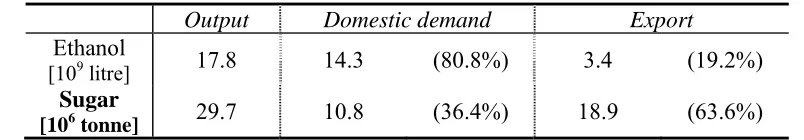
(6) 1. INTRODUCTION In response to oil price increases since 2000 and concerns about global warming, policies promoting biofuels are being investigated and implemented by many countries, including major energy users such as the USA, EU and Japan. In developed countries, such initiatives result mainly from concerns about the balance of trade, energy security and greenhouse gas emissions. Developing countries view biofuels in economic growth terms, seeing them as a means to improved energy access, higher income and employment, lower poverty and rural development. Recently, these interests have converged, making fuel ethanol a central issue in international energy policy debates. In this paper, we investigate the economic impacts of rapid growth in Brazilian ethanol exports and domestic consumption, using a disaggregated multi-regional computable general equilibrium (CGE) model with energy-industry detail. Brazil is the largest producer of sugarcane, sugar and ethanol from sugarcane1 in the world. In the 2006 crop, 430 million tonnes of sugarcane were harvested from an area of 6.3 million hectares; ethanol and sugar produced at 367 plants reached 17.8 billion litres and 29.7 million tonnes, respectively (Unica, 2007a). About 3.4 billion litres of ethanol were exported – mainly to US (51.2%%), Netherlands (10.1%), Japan (6.7%), Sweden (5.9%) and the so-called Caribbean Basin Initiative (CBI) countries2 (14.2%) – at an average fob price of US$ 0.45 (Datamark, 2007). Output, domestic demand and exports are summarized in Table 1. Table 1. Ethanol and sugar output, domestic demand and export in 2006. Output Ethanol. [109 litre]. Sugar [106 tonne]. Domestic demand. Export. 17.8. 14.3. (80.8%). 3.4. (19.2%). 29.7. 10.8. (36.4%). 18.9. (63.6%). Unica (2007b) expects ethanol and sugar output, domestic demand and exports in 2020 to be as shown in Table 2. Table 2. Ethanol and sugar output, domestic demand and export in 2020. Output Ethanol. [109 litre]. Sugar [106 tonne]. Domestic demand. Export. 65.3. 49.6. (76.0%). 15.7. (24.0%). 45.0. 12.1. (26.9%). 32.9. (73.1%). 1. In recent years US has surpassed Brazil in ethanol production. However in the US, ethanol is produced from maize. 2 Under the U.S.-Caribbean Basin Trade Partnership Act (CBTPA), CBI countries are able to export dutyfree anhydrous ethanol to the US. Exports are mostly hydrous ethanol is imported from Brazil to be processed in dehydration plants located in El Salvador, Jamaica, Costa Rica, Trinidad and Tobago, Nicaragua and Dominican Republic, among other CBI countries.. 2.

(7) According to Unica (2007b), also, in 2020 sugarcane production and crop area will be 1,038 million tonnes as 13.9 million hectares, respectively (Table 3). Table 3. Sugarcane production and crop area in 2006 and 2020.. Production [106 tonne]. Crop area [106 ha]. 2006. 2020. 430. 1,038. 6.3. 13.9. Unica (2007c) estimates that in 2006, sugarcane crop area corresponded to only 2.1% of total arable land in Brazil (nearly 300 million hectares), suggesting that it would not be difficult to convert part of grazing land (approximately 200–220 million hectares) for growing sugarcane. In fact, a study by Unicamp (2006) locates 12 large expansion areas in Brazil containing a total of 28.4 million hectares of land still available and suitable for growing sugarcane with productivity above 73.1 tonnes/ha without irrigation. Considering that 1.63 kg of sugar is equivalent to about one litre of ethanol3, total output indicated in Tables 1 and 2 may be expressed as shown in Table 4. Therefore, in the scenario proposed (Table 2), productivity is expected to grow at the conservative rate of 1.1% p.a. As indicated in Unica (2007c), improvements in the agricultural (e.g. genetically-modified sugarcane varieties) and industrial stages of the ethanol production chain and also new technologies involving the use of sugarcane trash (e.g. bagasse ethanol) are not being considered. Such productivity increases will lead ultimately to the reduction in land requirements. Table 4. Total output (ethanol-equivalent volume) and productivity in 2006 and 2020.. Output. [109 litre]. Productivit y. 2006. 2020. 36.0. 92.9. 5,710. 6,684. [litre/ha]. The introduction of flex-fuel vehicles (FFVs) in 2003 has been bringing about significant structural changes in the automotive and fuel markets in Brazil. Fuel choice by FFV drivers depends on the relative price of hydrous ethanol in terms of gaso-alcohol4. In general, whenever the relative price is lower than 0.7, ethanol will be preferred5. Since 2001, ethanol-gasoline relative prices have been in the 0.55–0.70 3. Conversion rate adopted by Sociedade dos Técnicos Açucareiros e Alcooleiros do Brasil (STAB); it applies for mills jointly producing sugar and ethanol. 4 The gasoline sold in fuel stations in Brazil is actually a blend of 20%–25% in volume of anhydrous ethanol and gasoline type A (pure gasoline). 5 Ethanol has lower energy content than gasoline. However, engines run more efficiently when the fuel used is ethanol.. 3.

(8) range over 80% of time. Since 2003, every time the price relationship has been unfavourable to ethanol (around 10% of time in the last four years), government has been called on to intervene in the ethanol market (Almeida et al., 2007). Total production of FFVs has reached more than 4 million. Currently, FFVs represent approximately 88% of sales of light-duty vehicles (LDVs) in Brazil. However FFVs constitute only about 20% of the current Brazilian fleet of 21.4 million LDVs. Hence the share of FFVs in the Brazilian LDV fleet is growing. By 2020, FFVs are predicted to account for more than 70% of a stock of almost 40 million LDVs (Petrobras, 2007). The domestic demand for ethanol is likely to grow steadily at a large rate, as indicated in Table 2. As we shall discuss in detail in Section 2, one part of our simulations involves modelling growth in the both the LDV fleet and the share of the fleet represented by FFVs. Table 5 summarises existing ethanol import tariffs implemented by major energyuser economies (Brenco, 2007). These are high. However, it is generally believed that, in the face of energy security and carbon emission concerns, such large barriers to ethanol trade will not continue beyond the near future. Hence Brazil, as the largest ethanol producer and exporter in the world, can also expect growing foreign demand for ethanol exports. In Section 2, we model the effects of growth in world demand for Brazilian ethanol. Table 5. Effective or equivalent ad valorem tariffs on ethanol imports. EU 63%. China 40%. US 39%. India 30%. Japan 27%. 2. SIMULATIONS 2.1 Simulation design The model and its underlying database incorporates many features of ethanol production in Brazil – including regional differences in ethanol and sugar production technologies, sugarcane harvesting methods, among others – which are expected to influence the adjustment of Brazil’s regional economies to a substantial expansion in ethanol production. We model three sources of expansion in Brazilian ethanol production: (i) growth in foreign demand; (ii) an increase in the share of flex-fuel vehicles in the private transport services (PTS) vehicle fleet; and (iii) growth in household vehicle ownership. The model contains 51 industries and 83 commodities. We have introduced six industries we think are important to modelling ethanol-related issues: manual cane harvesting, mechanical cane harvesting, sugar-ethanol plants, ethanol distilleries, ethanolgasoline blending and private transport services (PTS). These industries produce cane, sugar, ethanol, gaso-alcohol and transport services. The sugar-ethanol industry is a jointproduct industry, producing sugar and ethanol with constrained ability to transform production between the two. PTS uses capital (LDVs), various fuel types, and other carrelated inputs, to produce transport services for households. Our simulations are conducted under a standard long-run closure. We assume that the national unemployment rate, participation rate, and hours worked per worker will not 4.

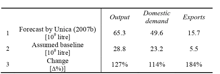
(9) be affected by our ethanol demand shocks. As a result, national employment rate is exogenous. Industry-specific capital stocks are free to adjust at given rates of return. Investment by each industry is determined via an assumption of fixed industry-specific investment/capital ratios. Consumption (private plus public) adjusts to maintain a given balance of trade to GDP ratio. Our land supply closure reflects anticipated regulatory environments. Although less than 45% of sugarcane is collected mechanically in São Paulo, a recent protocol established between the state government and sugar and ethanol producers requires phasing out of manual harvesting by 2014 (Unica, 2007d). Similar regulations are likely to be adopted in other regions. However, given the importance of manual harvesting in many regions, the extent of nation-wide enforcement of such regulations by 2020 is hard to predict with much certainty. We adopt a middle-position. We hold fixed the quantity of land available to manual cane harvesting, but allow the industry to continue to operate under this fixed land constraint. Hence, additional production by this method is possible, but only by increasing the intensity of variable factor (labour and capital) use with the given supply of manual harvest land. As we shall see, this will change the functional income distribution between labour, capital and land. Moreover, land that is currently suitable for manual harvesting will experience a significant price increase as it becomes relatively scarcer. In contrast, we allow land supply to mechanical cane harvesting to expand. This occurs via movement of land out of other agriculture and into mechanical cane harvesting. We hold fixed the total supply of land available to all forms of agriculture. As we shall see, the movement of land out of other agriculture and into mechanical harvesting proves to be modest. Our model allows ethanol to be produced by distilleries and combined sugarethanol plants (hereafter referred to as mills). For mills, sugar and ethanol have a jointproduct nature. Our early simulations showed that to allow mills to expand ethanol production under current joint-production technology has a severe impact on the sugar refining industry. That is, growing sugar production by mills dramatically depresses sugar prices, causing sharp contraction in sugar refining activity. We counteract this in two ways. Firstly, we allow users of sugar to treat sugar produced by different technologies to be close, but not perfect, substitutes. Secondly, we allow a revenue-neutral twist in the production possibility frontier of the combined sugar-ethanol plants, allowing them to expand ethanol output while holding sugar output unchanged. As we shall see, this allows much of the expansion of ethanol production to derive mainly from distilleries – and not from mills. The shocks imposed on key model variables are based on Tables 1 and 2, and summarised by row (3) of Table 6. Row (1) of Table 6 reproduces year 2020 forecasts by Unica (2007b) for ethanol output, domestic demand and exports (see Table 2 for details). We think ethanol forecasts (Table 2) can be divided into two parts: (i) a part due to baseline growth in the Brazilian economy; and (ii) a part due to rapid growth (above baseline GDP growth) of the ethanol industry. We determine baseline growth by assuming levels will grow from the values observed in 2006 (Table 1) at projected GDP growth rate of 3.5% p.a.6. The resulting baseline ethanol output, domestic demand and export values are reproduced in row (2) of Table 6. We interpret the difference between 6. Growth rate for GDP of 3.5% p.a. is the approximate average of the values corresponding to scenarios B1 and B2 by EPE (2007).. 5.

(10) rows (2) and (1) as that due to rapid growth in the ethanol sector. In that sense, row (3) may be understood as shocks applied to the projected 2020 Brazilian economy.7 Evidently, the effects arising from these shocks will be experienced progressively over the period 2006–2020. Table 6. Derivation of shocks.. 1 2 3. Forecast by Unica (2007b) [109 litre]. Assumed baseline [109 litre]. Change [∆%)]. Output. Domestic demand. Exports. 65.3. 49.6. 15.7. 28.8. 23.2. 5.5. 127%. 114%. 184%. We undertake our simulations in two steps. In Step 1, we derive the shifts in structural features of the Brazilian economy that are necessary to meet forecasts by Unica (2007b) for rapid growth in the ethanol industry. As we shall see, these structural features are: (i) foreign willingness to pay for Brazilian ethanol, that is, the vertical position of the Brazilian ethanol export demand schedule; (ii) ethanol/gaso-alcohol input proportions in the private transport services industry; and (iii) household preference for private transport services. In Step 2, we examine the individual contributions to Brazilian economic outcomes of the above three structural shifts. We implement the Step 1 shocks as follows: (a) To accommodate ethanol export forecast by Unica (2007b), we exogenise ethanol exports and endogenise the vertical position of the foreign demand schedule for Brazilian ethanol. Under this closure, Unica’s rapid export growth forecast is explained by growing foreign demand for Brazilian ethanol. (b) To accommodate ethanol output forecast by Unica (2007b), we exogenise Brazilian ethanol output, and endogenise the PTS sector’s ethanol input requirements. Under this closure, rapid growth in Brazilian ethanol production is explained by both growth in ethanol exports (see (a) above) and by a shift in PTS fuel requirements towards ethanol. We neutralise the impact of the increase in PTS ethanol input requirements on PTS unit costs by implementing a simultaneous cost-neutral reduction in PTS gaso-alcohol requirements. We interpret this cost-neutral shift in PTS input requirements (away from gaso-alcohol and towards ethanol) as an increase in the share of flex-fuel vehicles in the Brazilian private passenger vehicle fleet. (c) Since PTS has a high expenditure elasticity, we anticipate growth in the Brazilian private passenger vehicle fleet in excess of real GDP growth out to 2020, our solution year. To reflect income-driven growth in PTS demand above baseline real GDP 7. This shock setting allows the database to be treated as atemporal, although the economic flows it contains refer to the year of 2002. Results obtained in the model can be interpreted then as the cumulative deviations from baseline by 2020 that arise from the above-baseline structural shifts that are responsible for Unica’s high ethanol output and demand forecasts.. 6.

(11) growth, we implement an 8% autonomous increase in household demand for PTS via a shock to the household preference for this commodity. Under the Step 1 closure, the above shocks allow the model to solve for movements in structural features of the Brazilian economy relating to ethanol demand, in particular: (i) foreign willingness to pay for Brazilian ethanol; and (ii) ethanol/gaso-alcohol input proportions in the private transport services industry. In our Step 2 simulation, we shock the above two sets of structural variables by the values computed in Step 1 and implement again the 8% positive shock to household demand for PTS services. Obviously, Step 2 reproduces the results of Step 1; however, by implementing as shocks the three sets of structural shifts responsible for our results in the Step 1 simulation, we are able to decompose the results of Step 1 into the individual contributions of each of the three sets of exogenous shocks8. Tables 7–9 report our results, identifying the contributions of the three sets of shocks as follows: (a) Export growth – this column reports the impact of growth in world demand for Brazilian ethanol. (b) Flex-fuel – this column reports the impact of PTS input requirements shifting, in a cost-neutral fashion, towards ethanol usage and away from gaso-alcohol usage. (c) PTS – this column reports the impact of the shift in household preferences towards PTS. We now proceed to discuss our simulation results. We examine the results column by column and also provide cross-column comparisons for important results. 2.2 Export growth In our Step 1 simulation, in which we impose forecasts by Unica (2007b) on the model while allowing structural features of the ethanol industry to accommodate, we found a 46% increase in the vertical position of the foreign demand schedule for Brazilian ethanol. When imposed as an exogenous shock in Step 2, this expansion in foreign demand for Brazilian ethanol has the effects reported in the first column of Tables 7–9. As is clear from column A of Tables 7–9, the impact on the Brazilian economy of growth in foreign demands for Brazilian ethanol is small. This reflects the still small share of Brazilian ethanol production that is destined for the export market. The most important macroeconomic consequences (Table 7) are a small rise in the terms of trade (row 18) which allows a small increase in real consumption spending (rows 1 and 3). The rise in the terms of trade allows the real balance of trade to move slightly towards deficit (rows 4 and 5). This requires a small appreciation of the real exchange rate (row 17). Turning to the industry results, reported in Table 8, we can see that the small real appreciation creates a small Dutch disease effect, revealed as contractions in output of trade-exposed mining and manufacturing sectors. The activity levels of mills (row 19) and distilleries (row 20) expand in direct response to the increase in foreign demand for ethanol. Since mills must respond to conditions in both the sugar and ethanol markets, the expansion in their activity is lower than that of distilleries, which produce only ethanol.. 8. We do this using the decomposition algorithm of Harrison et al. (2000), which is automated by the Gempack software (Harrison and Pearson 1996) that we use to solve the model.. 7.

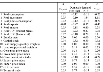
(12) Table 7. National macroeconomic variables (% change from 2006 levels attributable to above-baseline growth). A. 1 2 3 4 5 6 7 8 9 10 11 12 13 14 15 16 17 18. Real consumption Real investment Real public consumption Real exports Real imports Real GDP (market prices) Real GDP (factor cost) Employment Capital stock Land supply (quantity weights) Land supply (rental weights) Consumer price index Investment price index Government price index Export price index Import price index GDP deflator Terms of trade. B. C. Domestic demand Export Flex-fuel PTS 0.02 –0.12 –0.11 0.05 –0.10 1.64 0.02 –0.12 –0.11 –0.01 –0.97 0.57 0.05 –0.18 0.40 0.02 –0.22 0.27 0.02 –0.18 0.28 0.00 0.00 0.00 0.04 –0.32 0.59 0.00 0.00 0.00 0.01 0.19 0.03 0.06 0.34 –0.15 0.04 0.45 –0.13 0.08 –0.18 –0.14 0.05 0.77 –0.15 0.00 0.00 0.00 0.07 0.37 –0.16 0.05 0.77 –0.15. D. Total –0.20. 1.58 –0.20 –0.40. 0.28 0.08 0.11 0.00 0.32 0.00 0.23 0.26 0.36 –0.24 0.68 0.00 0.28 0.68. Table 8. National industry variables (% change from 2006 levels attributable to above-baseline growth). A. Export 1 2 3 4 5 6 7 8 9 10 11 12 13 14. Manual harvest sugarcane Machine harvested sugarcane Other agriculture, forestry and fishing Mining and quarrying Petroleum and gas extraction Non-metallic mineral products Iron and steel Non-ferrous metals Fabricated metal products Machinery, tractors and equipment Electrical machinery Office, accoun'g and comput'g machinery Motor vehicles Other vehicles and automotive parts. 0.70 4.83 –0.03 –0.19 –0.04 0.00 –0.11 –0.11 –0.06 0.00 –0.02 –0.06 –0.08 –0.25. B. C. D. Domestic demand Total Flex-fuel PTS 26.91 1.78 29.39 118.57 13.66 137.06 –0.68 –0.42 –1.14 –3.31 0.88 –2.62 –5.91 1.19 –4.76 –0.88 0.81 –0.07 –1.54 1.10 –0.54 –1.49 0.72 –0.88 –1.00 0.81 –0.25 0.25 0.98 1.23 –0.86 0.18 –0.70 –0.82 0.04 –0.84 –0.72 3.65 2.84 –2.50 1.67 –1.07. 8.

(13) 15 16 17 18 19 20 21 22 23 24 25 26 27 28 29 30 31 32 33 34 35 36 37 38 39 40 41 42 43 44 45 46 47 48 49 50 51. Wood and wood products Pulp, paper, paper prods, print'g and publ'g Rubber products Sugar refining Sugar-ethanol plants Ethanol distilleries Other chemicals (excluding pharmaceuticals) Coke and refined petroleum Fertilisers and other chemicals Pharmaceuticals Plastic products Textiles Clothing products Footwear products Coffee products Other vegetable processing Meat Dairy products Vegetable oil mills Other food products Miscellaneous manufacturing Electricity from bagasse Other electricity Electricity distribution Gas and water supply Construction Gasoline/ethanol blend Wholesale and retail trade Transport Post and telecommunications Finance and insurance Personal services Business services Dwellings services Public administration Private households with employed persons Private transport services. –0.07 –0.03 –0.06. –1.22 –0.62 –1.68. 0.45 1.72 3.08 –0.06 0.01 0.04 0.02 –0.02 0.00 0.02 –0.28 –0.07 –0.05 –0.06 –0.01 –0.03 –0.03 –0.06 0.02 –0.02 –0.01 0.11 0.05 0.03 0.01 –0.02 0.01 0.00 0.01 –0.04 0.03 0.02 0.01 0.02. 11.86 49.55 93.53 –1.24 –5.89 1.27 –0.47 –1.48 –0.35 –0.13 –4.54 –1.11 –0.80 –1.00 –0.46 –0.62 –0.62 –0.75 1.85 –1.12 –0.93 2.09 –0.22 –39.87 –1.39 –1.35 –0.35 –0.53 –0.15 0.08 –0.38 –0.10 0.10 1.01. 0.32 0.02 0.96 2.11 4.80 7.90 0.43 1.12 0.27 –0.98 0.43 –0.24 –0.97 1.01 –0.18 –0.61 –0.55 –0.76 –0.62 –0.70 0.04 –0.46 –0.18 –0.21 –1.38 1.02 4.30 0.19 –0.01 –0.48 0.28 –0.63 0.34 –0.98 –0.11 –1.09 6.19. –0.97 –0.63 –0.79. 14.42 56.07 104.51 –0.87 –4.76 1.58 –1.43 –1.07 –0.59 –1.08 –3.80 –1.36 –1.46 –1.60 –1.23 –1.27 –1.34 –0.76 1.41 –1.31 –1.15 0.83 0.84 –35.53 –1.19 –1.38 –0.82 –0.25 –0.77 0.38 –1.32 –0.19 –0.97 7.22. Among the agricultural sectors, only manual and mechanical cane harvesting expand. This reflects their supply of intermediate inputs to mills and distilleries. Expansion in manual cane harvesting (row 1) is far less than that of mechanical cane harvesting (row 2). This reflects our assumption of fixed land supply to manual cane harvesting, which limits the ability of this sector to expand in response to rising cane prices. We assume that movements in relative land prices induce land to move between mechanical cane and other agriculture. Expansion in mechanical cane activity causes the price of land used in mechanical cane to rise. This causes a change in land usage, away from other agriculture and towards mechanical cane harvesting. While not reported in 9.

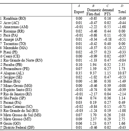
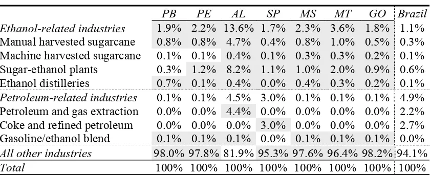
(14) Tables 7–9, this change in land usage is small for export growth – land usage in mechanical cane rises by 4.4%, and falls in other agriculture by 0.07%. Table 9. Real gross regional product (% change from 2006 levels attributable to above-baseline growth). A. 1 2 3 4 5 6 7 8 9 10 11 12 13 14 15 16 17 18 19 20 21 22 23 24 25 26 27. Rondônia (RO) Acre (AC) Amazonas (AM) Roraima (RR) Pará (PA) Amapá (AP) Tocantins (TO) Maranhão (MA) Piauí (PI) Ceará (CE) Rio Grande do Norte (RN) Paraíba (PB) Pernambuco (PE) Alagoas (AL) Sergipe (SE) Bahia (BA) Minas Gerais (MG) Espírito Santo (ES) Rio de Janeiro (RJ) São Paulo (SP) Paraná (PA) Santa Catarina (SC) Rio Grande do Sul (RS) Mato Grosso do Sul (MS) Mato Grosso (MT) Goiás (GO) Distrito Federal (DF). B. C. Domestic demand Export Flex-fuel PTS 0.00 –0.65 0.16 0.01 –0.47 0.02 –0.01 –2.22 0.55 0.02 –0.46 0.44 –0.01 –0.68 0.11 0.01 –0.34 –0.18 0.01 –0.42 0.40 0.01 –0.37 0.13 0.02 –0.57 0.23 0.00 –0.99 0.02 0.01 –1.33 0.47 0.10 1.94 0.32 0.07 1.39 0.27 0.35 9.37 1.15 0.02 –1.02 0.47 0.00 –1.86 0.38 0.00 –0.46 0.39 –0.01 –0.74 0.36 –0.01 –2.17 0.04 0.04 0.74 0.36 0.03 0.19 0.27 –0.02 –0.84 0.15 –0.03 –1.24 0.19 0.07 1.70 0.26 0.09 2.37 0.29 0.06 1.23 0.37 0.01 –0.46 0.02. D. Total –0.49 –0.44 –1.68. 0.00 –0.58 –0.51 0.00 –0.22 –0.33 –0.97 –0.84 2.35 1.73 10.87 –0.53 –1.49 –0.08 –0.39 –2.14 1.14 0.49 –0.71 –1.08 2.03 2.75 1.66 –0.43. At the regional level, the main beneficiaries of growth in foreign ethanol demand are Alagoas, Mato Grosso, Paraíba, Mato Grosso do Sul, Pernambuco, Goiás and São Paulo (Table 9). This reflects the varying importance of different cane harvesting and ethanol production technologies in these regions. We reinforce this idea by providing Tables 10 and 11, which reports industry value added shares in regional GDP for selected regions and industries. We shade in grey those regional industries that account for higher shares of regional value added than is the case nationally. For example, Alagoas experiences the largest expansion in real GDP in column A. This is due to growth in output of manual cane harvesting and mills. Manual harvesting and mills account for approximately 5% and 8% respectively of Alagoas’ value added, while accounting for 10.

(15) only 0.3% and 0.6% respectively of national GDP (Table 10). Interestingly, of the industries most affected by expansion in ethanol production, these two industries are the most constrained: (i) manual harvesting via fixed land supply; and (ii) mills via its joint product nature. However, both industries account for very high shares of Alagoas’ value added. Hence, despite experiencing small output gains relative to mechanical harvesting and distilleries, the high shares of Alagoas’ activity explained by manual harvesting and mills is sufficient to lift this region to the top of the real regional GDP rankings. The remaining top ranked regions in column A of Table 9 are also the regions for which we report selected industrial value added shares in Table 10. From Table 10 it is clear that ethanol-related industries account for comparatively high shares of activity in these regions. This explains the high GDP increases of these regions. Table 10. Industrial shares in regional GDP (at factor cost), for selected ethanoloriented regions.. Ethanol-related industries Manual harvested sugarcane Machine harvested sugarcane Sugar-ethanol plants Ethanol distilleries Petroleum-related industries Petroleum and gas extraction Coke and refined petroleum Gasoline/ethanol blend All other industries Total. PB 1.9% 0.8% 0.1% 0.3% 0.7% 0.1% 0.0% 0.0% 0.1% 98.0% 100%. PE 2.2% 0.8% 0.1% 1.2% 0.1% 0.1% 0.0% 0.0% 0.1% 97.8% 100%. AL 13.6% 4.7% 0.4% 8.2% 0.4% 4.5% 4.4% 0.0% 0.1% 81.9% 100%. SP 1.7% 0.4% 0.1% 1.1% 0.0% 3.0% 0.0% 3.0% 0.0% 95.3% 100%. MS 2.3% 0.8% 0.3% 1.0% 0.4% 0.1% 0.0% 0.0% 0.1% 97.6% 100%. MT 3.6% 1.0% 0.3% 2.0% 0.3% 0.1% 0.0% 0.0% 0.1% 96.4% 100%. GO 1.8% 0.5% 0.2% 0.9% 0.2% 0.1% 0.0% 0.0% 0.1% 98.2% 100%. Brazil 1.1% 0.3% 0.1% 0.6% 0.1% 4.9% 2.2% 2.7% 0.0% 94.1% 100%. PB – Paraíba, PE – Pernambuco, AL – Alagoas, SP – São Paulo, MS – Mato Grosso do Sul, MT – Mato Grosso, GO – Goiás; shading denotes that the industry's share in regional GDP is higher than the national average.. 2.3 Domestic growth – flex-fuel vehicles In Step 1, the simulation in which we exogenously impose ethanol production and export targets on the model, we found that export growth alone was insufficient to account for high ethanol production forecasts by Unica (2007b). To accommodate these forecasts, we also required a shift in PTS input requirements towards ethanol. We view this as reflecting growth in the share of flex-fuel vehicles in the PTS capital stock. Hence we assumed that the shift in PTS inputs towards ethanol would be matched by a costneutral shift in input requirements away from gaso-alcohol. In our Step 2 simulation, we impose these shifts in PTS input requirements as exogenous shocks. The impacts of these shifts in PTS input technology – away from gaso-alcohol and towards ethanol – are reported in column B of Tables 7–9. The effects of the shift in PTS fuel input requirements are best understood by beginning with the industry results, reported in Table 8. Here, the effect of reduced gasoalcohol usage is immediately clear, with the blending sector (row 41) contracting by almost 40%. At the same time, ethanol producing industries (rows 19 and 20) expand. This simply reflects the shift in PTS fuel requirements away from gaso-alcohol (produced 11.

(16) by sector 41) towards ethanol (produced by sectors 19 and 20). This has no direct effect on output of PTS (row 51) because, by design, the input switch is cost neutral. Looking across the columns of rows 19 and 20, it is clear that growth in domestic demand – via increasing flex-fuel car ownership (column B) and growth in PTS demand in general (column C) – accounts for the bulk of forecast by Unica (2007b) for rapid growth in the ethanol production sectors. In comparison, growth in world demand for Brazilian ethanol (column A) looks relatively unimportant. The shift in fuel usage, away from gaso-alcohol towards ethanol, also has impacts on upstream industries. Expansion of the ethanol production industries (rows 19 and 20) causes output of cane harvesting sectors (rows 1 and 2) to expand. Expansion of mechanical cane harvesting (row 2) causes some movement of land out of other agriculture (row 3), causing output of other agriculture to contract. The contraction in other agricultural that is necessary to facilitate expansion of mechanical cane harvesting is small, at 0.7%. Land usage by other agriculture contracts by 1.7%, as land use switches to mechanical harvesting. This contributes to contraction of downstream food processing industries (sectors 29–34). Some food processing sectors are also adversely affected by real appreciation (see next paragraph). In particular, approximately half the output contraction of such export-oriented food processing sectors as coffee products (sector 29), other vegetable processing (sector 30), meat (sector 31), vegetable oil mills (sector 33) and other food products (sector 34) is due to real appreciation. Contraction in the gaso-alcohol industry causes output of petroleum refining (row 22) and petroleum and gas extraction (row 5) to fall. However the potential falls in output of these two upstream industries is mitigated by export expansion. As domestic demand for gasoline declines, much of the resulting surplus is taken up by expansion in exports. This reflects our assumption that Brazil faces high export demand elasticities for petroleum products. As a result of expanded petroleum exports, exports of other commodities for which Brazil has more market power are able to decline. It is the decline in other exports that accounts for the terms of trade gain in Table 7 (row 18, column B). For non-gasoline exports to contract, the real exchange rate must appreciate. This accounts for the rise in the real exchange rate in Table 7 (row 17, column B). This explains the contraction of export and import competing sectors such as mining and quarrying (row 4), machinery, tractors and equipment, electrical machinery, office machinery, motor vehicles, other vehicles and automotive parts, wood and wood products, pulp, paper, paper prods, print’g and publ’g and rubber products (rows 10–17), plastic products (row 25), textiles (row 26), footwear products (row 28) and miscellaneous manufacturing (row 35). The adjustment mechanism constitutes an indirect Dutch disease effect resulting from exports of oil substituted by ethanol in the domestic market. Growth in the flex-fuel vehicle stock causes Alagoas, Mato Grosso, Paraíba, Mato Grosso do Sul, Pernambuco, Goiás, São Paulo and Paraná to expand. These regions share the characteristic that cane harvesting and ethanol production industries represent comparatively high shares of total regional value added (see Table 10). Hence expansion of the cane harvesting and processing sectors has the largest regional GDP outcomes in these regions. However output expansion in São Paulo is somewhat constrained by real appreciation. As discussed above, real appreciation has an adverse impact on output of export and import competing industries. Compared to the Brazilian economy taken as a whole, these industries represent a relatively high share of São Paulo’s GDP.. 12.

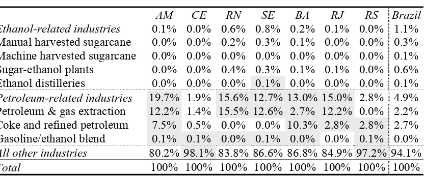
(17) Growth in the flex-fuel share of the PTS sector causes all other regions to contract. The largest contractions are experienced by Amazonas (–2.2%), Rio de Janeiro (–2.2%), Bahia (–1.9%), Rio Grande do Norte (–1.3%) and Rio Grande do Sul (–1.2%). All five regions share the characteristic that little or none of their regional GDP is attributable to value added in cane harvesting and processing industries (see Table 11). Hence they gain little from the expansions of sectors such as manual and mechanical cane harvesting, sugar-ethanol plants and distilleries. At the same time, they have varying degrees of exposure to the contracting petroleum extraction and refining industries. Amazonas, Rio de Janeiro and Bahia have above-average shares of their regional activity in petroleum and gas extraction and petroleum refining. Hence they are adversely affected by the contraction of these sectors. A high proportion of Rio Grande do Norte’s GDP is attributable to value added in the petroleum and gas extraction industry. Table 11. Industrial shares in regional GDP (at factor cost), for selected petroleumoriented regions.. Ethanol-related industries Manual harvested sugarcane Machine harvested sugarcane Sugar-ethanol plants Ethanol distilleries Petroleum-related industries Petroleum & gas extraction Coke and refined petroleum Gasoline/ethanol blend All other industries Total. AM 0.1% 0.0% 0.0% 0.0% 0.0% 19.7% 12.2% 7.5% 0.1% 80.2% 100%. CE 0.0% 0.0% 0.0% 0.0% 0.0% 1.9% 1.4% 0.5% 0.1% 98.1% 100%. RN 0.6% 0.2% 0.0% 0.4% 0.0% 15.6% 15.5% 0.0% 0.0% 83.8% 100%. SE 0.8% 0.3% 0.0% 0.3% 0.1% 12.7% 12.6% 0.0% 0.1% 86.6% 100%. BA 0.2% 0.1% 0.0% 0.1% 0.0% 13.0% 2.7% 10.3% 0.0% 86.8% 100%. RJ 0.1% 0.0% 0.0% 0.1% 0.0% 15.0% 12.2% 2.8% 0.0% 84.9% 100%. RS 0.0% 0.0% 0.0% 0.0% 0.0% 2.8% 0.0% 2.8% 0.1% 97.2% 100%. Brazil 1.1% 0.3% 0.1% 0.6% 0.1% 4.9% 2.2% 2.7% 0.0% 94.1% 100%. AM – Amazonas, CE – Ceará, RN – Rio Grande do Norte, SE – Sergipe, BA – Bahia, RJ – Rio de Janeiro, RS – Rio Grande do Sul; shading denotes that the industry's share in regional GDP is higher than the national average.. 2.4 Domestic growth – growth in the PTS sector Household demand for PTS services is income elastic. Hence we expect growth in PTS output to be greater than growth in real GDP. Dargay et al. (2007) estimate that by 2030, the six countries with the largest number of vehicles will be China, USA, India, Japan, Brazil and Mexico; stock of road vehicles in Brazil is projected to grow at an average annual rate of 5.1% between 2002 and 2030. As discussed in Subsection 2.1, we implement this as a shift in household preferences towards PTS. In Table 8, we can see this expressed as a rise in output of PTS (row 51, column C). This stimulates activity in the blending industry (row 41), the ethanol production industries (rows 19 and 20) and the refining industry (row 22). To maintain the new, higher level of PTS output, more cars are required. This accounts for the expansion of the automobile sector (row 13). Upstream industries, such as motor vehicles parts (row 14), cane harvesting (rows 1 and 2) and petroleum and gas extraction (row 5) also expand. At the national level, aggregate investment rises relative to real GDP. This reflects the high investment/capital ratio of the PTS sector. Ceteris paribus, the rise in real 13.

(18) investment pushes the balance of trade towards deficit. However, we hold the balance of trade to GDP ratio exogenous via adjustment of real consumption. This explains the reductions in real private and public consumption in column C of Table 7. Service-oriented regions tend to be lowly ranked in column C of Table 9. This is so for two reasons. Firstly, the shock is a shift in household tastes towards PTS. Since household budget constraints are not directly affected by taste changes, the shift in tastes towards PTS must simultaneously be a movement in household tastes away from all other consumption goods. Since services figure prominently in the household budget, this has an adverse impact on regions that are specialised in service provision. Secondly, as discussed above, the macroeconomic closure requires real private and public consumption to fall. Regions with high shares of regional GDP in adversely affected sectors such as personal services and public administration include Amapá, Ceará, Acre and Distrito Federal.. 3. CONCLUSIONS In this paper, we investigated the effects of rapid growth in the Brazilian ethanol industry. We defined rapid growth as growth above real GDP growth. We traced the causes of rapid growth in Brazilian ethanol to three causes: (i) export growth; (ii) growth in the flex-fuel vehicle share of the domestic light duty fleet; and (iii) growth in private use and ownership of motor vehicles. Debate on the prospects for the Brazilian ethanol industry often places a high weight on export growth. Yet, in our simulations, we find that growth in domestic ethanol demand will be the major influence on the Brazilian ethanol industry, at least to 2020. Growth in ethanol production requires cane harvesting to expand. For manual cane harvesting, we assumed this will only be possible through more intensive use of land where cane is already harvested manually. For mechanical cane harvesting, we allow land to move from other agricultural uses. Only a small (2%) reduction in land use by other agriculture is necessary to accommodate the required expansion in mechanical harvesting. We find that rapid growth in ethanol production causes contractions in output by food processing sectors. These contractions are small – by 2020 of the order of –1.5% relative to what output would otherwise have been. One cause of the small contraction in food processing is the flow of land out of other agriculture. This places upward pressure on food processing input costs. However, for most food processing sectors, two other effects are of equal or greater importance. Firstly, many food processing sectors are tradeexposed via significant export sales. Growth in the flex-fuel vehicle stock causes oil exports to expand, crowding out other exports via appreciation of the real exchange rate. Real appreciation has an adverse effect on output of trade-exposed food processing sectors. Secondly, within a given budget constraint, growth in household demand for PTS must come at the expense of private consumption of other commodities. The food processing sectors sell high shares of their output to private consumption. We see our results as being sensitive to three assumptions in particular, and in future work we hope to explore these assumptions further. The three assumptions are: fixed national agricultural land supply; shifts in mill production technology towards. 14.

(19) ethanol output; and continuation of manual harvesting, but under fixed manual harvest land supply. We expand on these issues below. We held national agricultural land supply fixed in our simulations. In policy debates on this issue, pressure for further land clearance is often associated with the rapid ethanol growth scenario. However we found that the amount of land that must shift from other agriculture to mechanical harvesting is small, relative to the amount of land presently used in other agriculture. The joint product nature of sugar and ethanol production by mills posed an issue for the sugar refining sector. In early simulations we found that this sector was hit hard by the sugar by-product produced by an expanded mills industry. To counteract this, we twisted the joint production technology of the mills industry towards ethanol. We think this is a strong assumption, and one we would like to explore further in future research. Our model allows for no further expansion in manual cane harvesting, but not its elimination. We find that Alagoas is a major beneficiary of rapid growth in ethanol demand. Part of this is due to growth in output of manual cane (despite fixed land supply). This sector is important to the Alagoas economy, accounting for almost 4.7% of the region’s GDP. Tight enforcement of a nation-wide ban on manual harvesting could reduce this region’s ability to participate in the benefits of growth in ethanol production. In future research we intend to explore this possibility by examining ethanol growth impacts using a database calibrated more to the structure of the 2020 economy than the 2002 economy. This would allow us to reduce (or even eliminate) manual cane harvesting from the base-case, facilitating an assessment of the regional consequences of growth in ethanol demand under a scenario of enforced bans on manual harvesting. The results in this paper suggest that the distribution of regional benefits would be quite different under these circumstances. This may need to be recognised by policy makers: if reducing the extent of manual cane harvesting remains a policy target, then, in an economic context of rapid growth in ethanol production, assistance for regions such as Alagoas may be needed.. ACKNOWLEDGEMENT The authors are grateful to Joaquim Bento de Souza Ferreira Filho for having provided an earlier version of the database.. REFERENCES Almeida, E. F., J. V. Bomtempo and C. M. Souza e Silva (2007). “The Performance of Brazilian Biofuels: An Economic, Environmental and Social Analysis.” Biofuels: Linking Support to Performance. International Transport Forum, Organisation for Economic Co-operation and Development (OECD), Paris, France. Brenco – Companhia Brasileira de Energia Renovável (2007). “Perspectivas de Investimentos em Bioenergia no Brasil” (H. P. Reichstul). Conferência Nacional de Bioenergia (Bioconfe), São Paulo, Brazil. (http://www.usp.br/bioconfe/palestras_pdf/Painel%204_Henri%20Philippe%20Reich stul_27.09.pdf). 15.

(20) Dargay, J., D. Gately and M. Sommer (2007). “Vehicle Ownership and Income Growth, Worldwide: 1960–2030.” The Energy Journal 28(4): 143–170. Datamark (2007). Foreign Trade Database. (http://www.datamark.com.br/administrator/secex/ComercioExterior.asp?lang=E) EPE – Empresa de Pesquisa Energética (2007). “Plano Nacional de Energia 2030.” (http://www.epe.gov.br/PNE/20071029_1.pdf) Harrison, W. J., J. M. Horridge and K. R. Pearson (2000). “Decomposing Simulation Results with Respect to Exogenous Shocks.” Computational Economics 15: 227–249. Harrison, W. J. and K. R. Pearson (1996). “Computing Solutions for Large General Equilibrium Models using Gempack.” Computational Economics 9: 83–127. Unica – União da Indústria de Cana-de-Açúcar (2007a). Estatísticas: Produção Brasil. (http://www.portalunica.com.br/portalunica/) Unica – União da Indústria de Cana-de-Açúcar (2007b). “Bioenergia e Indústria Automobilística no Brasil e no Mundo” (M. S. Jank). Conferência Nacional de Bioenergia (Bioconfe), São Paulo, Brazil. (http://www.usp.br/bioconfe/palestras_pdf/Painel%206_Marcos%20Jank_28.09.pdf) Unica – União da Indústria de Cana-de-Açúcar (2007c). “Panorama do Mercado Global de Etanol” (M. S. Jank). Bolsa de Mercadorias & Futuros (BM&F), Rio de Janeiro, Brazil. (http://www.bmf.com.br/portal/pages/imprensa1/destaques/2007/outubro/MarcosJAN K.pdf) Unica – União da Indústria de Cana-de-Açúcar (2007d). “Bionergia e Meio Ambiente” (A. Szwarc). Conferência Nacional de Bioenergia (Bioconfe), São Paulo, Brazil. (http://www.usp.br/bioconfe/palestras_pdf/Painel%205_Alfred%20Szwarc_28.09.pdf ) Unicamp – Universidade Estadual de Campinas (2006). Study on the Possibilities of and Impacts from Large Scale Production of Ethanol Aiming at the Partial Substitution of Gasoline in the World (in Portuguese). Final report, Centre for Management and Strategic Studies (CGEE), Brazilian Ministry of Science and Technology (MCT). Petrobras (2007). “Biocombustíveis e a Economia brasileira” (M. S. Queiroz). Conferência Nacional de Bioenergia (Bioconfe) , São Paulo, Brazil. (http://www.usp.br/bioconfe/palestras_pdf/Painel%204_Mozart%20S.%20de%20Que iroz_27.09.pdf). 16.

(21)

No results found