Hybrid Differential Evolution based
Concurrent Relay-PID Control for Motor
Position Servo Systems
B.Saritha
1, Dr. L. Ravi Srinivas
2P.G. Student, Department of EEE, Gudlavalleru Engineering College, Gudlavalleru, Andhra Pradesh, India1 Professor, Department of EEE, Gudlavalleru Engineering College, Gudlavalleru, Andhra Pradesh, India2
ABSTRACT: This paper presents the implementation of HDE algorithm for Concurrent Relay-PID (CRPID) controller for motor position servo systems. CRPID is composed of a deadband relay subcontroller which improves the transient performance and the parallel PID subcontroller which improves the steady state performance of the system. Controller is implemented using modern heuristic tuning techniques which are Differential Evolution (DE) and Hybrid Differential Evolution (HDE). The performance of these optimization techniques is evaluated by setting their objective function as Integral Square Error (ISE). Using both DE and HDE optimization techniques comparison of performance has been made between PID and CRPID.
KEYWORDS:PID, CRPID, DE, HDE, deadband relay, servo systems.
I. INTRODUCTION
Electrical servo systems are widely used in robotics, automated factories, electrical vehicles. PID controllers are simple in structure reliable in operation and robust in performance however, they may produce higher overshoots and over oscillatory responses. Hybrid scheme CRPID improves the system performance in terms of transient as well as steady state. CRPID is composed of two controllers one is conventional PID subcontroller which improves the steady state performance and another one is deadband relay subconroller which improves the transient performance of the system. The goal of PID controller tuning is to attain the optimal control parameters so as to meet the closed loop system performance specifications over a wide range of operating conditions. Improper PID control parameter tuning could lead to cyclic and slow recovery and poor robustness will be the collapse of system operation [1]. To obtain optimal control parameters of PID may strategies has been proposed. Among conventional PID tuning methods Zeigler-Nichols is most popular method however, this may produce large overshoot [2].
This paper is organised as fallows. Section II describes the proposed control strategy and section III describes the mathematical model of the plant. Section IV describes design pattern of two subcontrollers. Section V illustrates simulation result. Conclusion has been made in section VI.
II. CONTROLSTRATEGY
The block diagram of proposed controller CRPID has been shown in Fig. 3. Control strategy consists of two subcontrollers. The PID subcontroller is a conventional PID controller. The deadband relay, lead compensator and a auxiliary limited integrator makes up a deadband relay subcontroller. When the system has large error deadband relay automatically turns on and produces either positive or negative maximum controller output until its error becomes small. Whenever the error reaches deadband limit deadband relay automatically turns off and the corresponding output becomes zero and PID subcontroller alone handles the system regulation around the steady state. The limited integrator is to aid the PID subcontroller with near steady state regulation. The integrator in the PID subcontroller may not accumulate sufficient strength to maintain the system output due to fast response of the deadband relay subcontroller in the transient state after the deadband relay subcontroller switches off. Limited integrator provides an initial value for system regulation near the steady state where only the PID subcontroller is in effect. Inclusion of auxiliary limited integrator reduces the settling time. While designing the plant unavoidable modeling errors occurred this may lead the system unstable. Lead compensator improves the relative stability of the resultant closed loop system.
Fig. 1 Block diagram of CRPID
Here controllers are tuned by Differential and Hybrid Differential Evolution techniques and the comparison has been between these techniques. Tuning of controllers are briefly described in the design pattern which is in the following sections.
III.MATHEMATICALMODELOFTHEPLANT
Fig. 2 Block diagram of dc servo system Fig. 3 Time domain block diagram representation of dc servo system
Block diagram of dc servo system is shown in Fig.2 and the time domain block diagram is represented in Fig. 3. From figures
(
s
)
is the position and it can be controlled using concurrent relay PID controller by tuning the controller with different tuning techniques.)
1
(
1
)
(
)
(
2s
R
K
K
D
J
s
J
R
K
s
E
s
a b t m m m a t a m
WhereJm= motor equivalent inertia constant=30*10 -6
kgm2 Kb=back-emf constant=60*10-3vsrad-1
Kt=motor torque constant=17*10-3NmA-1
Ra=armature resistance=3.2Ω
Dm=motor equivalent viscous density =small (neglected)
La=armature inductance=small (neglected).
The open loop transfer function of the dc servo system is
) 2 ( 625 . 10 0833 . 177 ) ( ) ( ) ( 2 S S s E s s G a m
IV.DESIGNPATTERN
1. Design of PID subcontroller: Controller PID and CRPID are implemented using modern heuristic tuning techniques Differential Evolution (DE) and Hybrid Differential Evolution (HDE).
The transfer function of the controller is
)
3
(
*
)
(
Kd
s
s
Ki
Kp
s
G
p
Where Kp = proportional gain; Ki = Integral gain; Kd = Derivative gain.
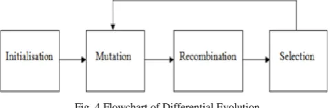
1.a. Differential Evolution: DE is a stochastic population based search technique. The algorithm has been used in many practical causes because of its good convergence and global optimization capability. DE can search for the optimal condition very fast with minimal control parameters such as initialization, mutation, crossover and selection. All these operations are briefly described in HDE technique. Mutation, crossover, selection continued until stoping criterion is reached as shown in Fig. 4. The main disadvantage of DE is premature convergence. HDE overcomes this limitation by performing migration operation.
Fig. 4 Flowchart of Differential Evolution
1.b. Hybrid Differential Evolution: Migration strategy is mainly added to original DE to perform Hybrid Differential Evolution by Chiou and Wang. HDE is an effective reliable optimization technique to obtain the optimum control parameters of the controller where the fitness value ISE is minimized [7].
Fitness Function:
Te
t
dt
ISE
0 2)
4
(
)}
(
{
Step 1. Initialization:
Initialize upper and lower bounds of each control variables and size of the population. The initial populations are chosen randomly in the interval [Xmin, Xmax] by uniform probability distribution. Fitness value has been calculated for
each set of control variables. Generation of control variables has been made using below formula.
max min
,
1
,....
(
5
)
min 0
p i
i
X
X
X
i
N
X
Where
i
[
0
,
1
]
is a random number. The initial process produces Np individuals of Xi0 randomly.Step 2. Mutation Operation:
Mutation expands the search space. A mutant vector is generated based on the present individual XiG as fallows
)
6
(
))
(
)
((
1 2 3 41 G r G r G r G r G i G
i
X
F
X
X
X
X
Y
The mutation factor was selected as
F
[
0
,
1
.
2
],
and the upper limit of 1.2 for F was determined empirically; r1, r2, r3and r4 are randomly selected and distinct.
Step 4. Crossover Operation:
Mutant vector YiG+1 and a present individual XiG are chosen by a binomial distribution to progress the crossover
operation to generate an offspring. The diversity of population has been increased. Each gene of the jth individual is reproduced from the mutant vector YiG+1 = (Y1iG+1, YG+12i, . . . ,YkiG+1) and the present individual XiG = (X1iG, X2iG, . . . ,
XkiG) . That is
)
7
(
,
,
1 1
otherwise
Y
C
number
random
a
if
X
Y
G hi r G hi G hiWhere i=1, 2, . . . , Np; h=1,2, . . . , nc; nc is the dimension of decision parameters; K is the no of genes; and the
crossover factor is set to be
C
r
[
0
,
1
]
.Step 4. Estimation and Selection:
The parent is replaced by its offspring if the fitness of the offspring is better than that of the parent. Contrarily, if the fitness of the offspring is worse than that of the parent then parent is retained for the next generation. Two forms are presented as follows
)
8
(
)
(
{
min
arg
&
)}
(
),
(
min{
arg
1 1 11
Gi G b G i G i G
hi
F
X
F
Y
X
F
X
X
Where arg min means the argument of the minimum and XbG+1 is the best individual.
Step 5. Migration If Necessary:
Migration strategy is to diversify a population that failed in certain tolerance besides escaping from local optimal and prevents premature convergence. The new populations are based on the best individuals XbG+1. The hth gene of the ith
individuals as fallows
) 9 ( ), ( ), ( 1 m ax 1 1 1 m ax m in 1 2 1 m in 1 1 1 otherwise X X X X X X X if X X X X G hb h G hb G hb h h G hi G hb h G hb G hi
Where
1,
2are randomly generated numbers uniformly distributed in the range of [0, 1]; h= 1, . . . , nc. The)
10
(
,
0
,
1
;
)
1
(
/
1 21 1 1 1 1
otherwise
X
X
X
if
X
N
n
X
G jb G jb G ji ji N b i i n j p c ji p c]
1
,
0
[
1
and
2
[
0
,
1
]
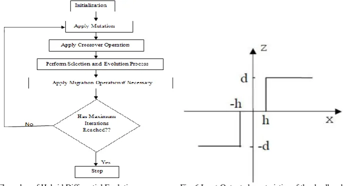
respectively express the desired steadiness for the population diversity and the gene diversity with respect to the best individual.Step 6. Repeat step 2 to step 5 until desired ISE is reached as shown in Fig. 5.
Fig. 5 Flow char of Hybrid Differential Evolution Fig. 6 Input-Output characteristics of the deadband relay
2. Design of Deadband Relay: The input-output characteristics of deadband relay have been shown in Fig. 6. From fig output is zero if the input of the deadband relay is within deadband limit and is positive or negative maximum controller output if deadband relay exceeds the threshold limit. Where d is the relay output amplitude and h represents the threshold value. Nonlinear systems can be analysed using describing function analysis.
Describing function of the deadband relay can be derived as [8, 9]
) 11 ( ) ( 1 4 ) ( 2 X h X d X
N
Where N(X): describing function of the deadband relay, d : relay output amplitude, h: half of the deadband width threshold, x represents input .
Inverse describing function of the deadband relay is
) 12 ( ) ( 1 4 ) ( 1 2 X h d X X N
It has a minimum value at some point in the admissible set of
X
:
{
X
X
h
}
. The minimum value of the inversedescribing function can be found at
X
2
h
. The threshold value must be selected in the rangemax
0
h
e
Where
:
maxe
maximum absolute error.The minimum value of the describing function is
) 13 ( 2 ) ( 1
m in d
3. Design of Limited Integrator: In order to reduce the settling time of the transient response of the system limited integrator is used after the deadband relay. Thepurpose of limited integrator is to complement the integrator already present in the PID subcontroller for fast settling-down of the system. Hence, the gain of the limited integrator should be some way related to the integral gain of the PID subcontroller.
Empirical formula for calculating the gain of the limited integrator is
) 14 ( 6
d K
K i
ai
Where
Kai: gain of the limited integrator, Ki : integral gain of the PID subcontroller.
Large gain could adversely affect the settling time of the entire system so diligence is always required while determining the gain of the limited integrator.
4. Design of Lead Compensator: The lead compensator is to improve the relative stability of the resultant closed loop system. The block diagram of the closed-loop system in terms of transfer functions /describing function is shown in fig. 7.
Fig. 7 Block diagram of closed loop system Fig. 8 Equivalent system for the design of lead compensator
Where Gc(s) : transfer function of the PID subcontroller, Gl(s) : transfer function of the lead compensator, Gp(s) :
transfer function of the plant, Gpi(s) : transfer function of pseudo-PI controller, N(X) : describing function of deadband
relay. The transfer function of the pseudo-PI controller following the deadband relay, which is given by
)
15
(
)
(
s
K
s
s
G
aipi
Figures 7 and 8 describes that the design of lead compensator for the deadband relay subcontroller is equivalent to the design of lead compensator for a plant with the transfer function of
)
1
(
)
(
1
m in
p c p pi
G
G
X
N
G
G
A lead compensator with unit static gain is of the form
) 16 ( )
1 0
( 1 1 )
(
TS TS s Gl
Where, T represents time constant of the numerator, α represents ratio of time constants.
V. SIMULATION RESULT
Let us consider positive /Negative maximum controller output is -2.2/2.2(volts). The output amplituse of the deadband relay is set to 2.2 volts due to the maximum controller output(d) is 2.2 volts and the threshold(h) of the deadband relay is considered as 0.15. the minimum value of the describing function for the deadband relay[10] is 0.107.
Tuning Ranges: Population=10, kpmin=0, kpmax=4, kimin= 0, kimax=2, kdmin=0, kdmax=0.5, Rate of crossover (cr)=0.8,
Mutation Factor( F)=0.5,
=0.2, lead=55deg.) 17 ( )
1 1 . 0 (
3 . 18 )
( ) ( ) (
S S s E
s s G
a m
Mathematical model is developed in [9] and the optimal control parameters of the controller are obtained by Hybrid Differential Evolution optimization technique. Control parameters obtained using ZN method for both PID and CRPID are kp=0.85; ki=2.83; kd=0.057.
Optimal control parameters for PID with HDE technique are kp=0.855; ki=2; kd=0.0706 and CRPID with HDE technique are kp=3.3075; ki=1.2284; kd=0.1233 and lead=55deg.
Fig. 9 Step responses of PID with ZN and HDE
Fig. 9 shows that the performance has been improved by tuning PID controller with HDE optimization technique. Overshoot decreases compared with ZN method.
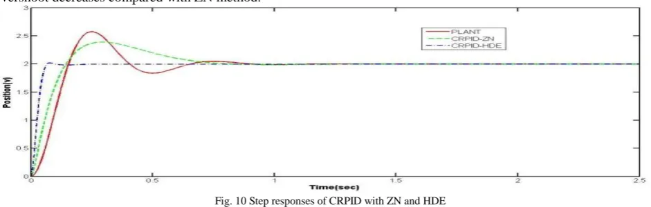
Fig. 10 Step responses of CRPID with ZN and HDE
Fig. 10 shows that the performance has been improved by tuning CRPID with HDE optimization technique an all control aspects like settling time, rise time, peak overshoot and steady state error. Hence CRPID is more effective compared with PID.
Case B:The transfer function of dc servo motor is represented by
) 18 ( 625
. 10
0833 . 177 ) (
) ( )
( 2
S S
s E
s s G
a m
Fig. 11 Convergence graphs of PID, CRPID with DE and HDE tuning techniques.
Fig 11 shows that minimization of ISE with no of iterations. ISE converges fast by tuning controllers with HDE technique and especially with CRPID.
Fig. 12 Frequency response of lead compensator with DE Fig. 13 Frequency response of lead compensator with HDE
Fig 12 and 13 shows the frequency response of lead compensator with DE and HDE. Relative stability has been greatly improved while tuning CRPID with HDE optimization technique.
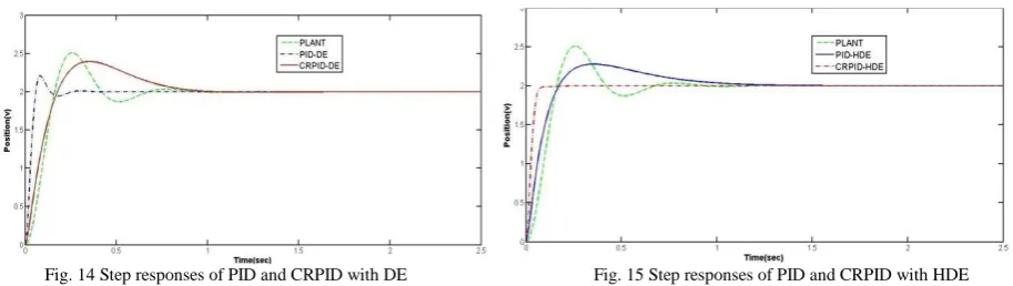
Fig. 14 Step responses of PID and CRPID with DE Fig. 15 Step responses of PID and CRPID with HDE
Tab. 1: Characteristics of step response with ISE objective function
Parameter Specifications PID-DE PID-HDE CRPID-DE CRPID-HDE
KP 0.7235 0.8073 4 3.1779 KI 2 1.8164 1.8898 1.2126 KD 0.0446 0.0581 0.0772 0.1274 Rise Time(sec) 0.1273 0.1193 0.0402 0.0437 Settling Time(sec) 0.8451 0.9755 0.2089 0.0734 Peak Overshoot(%) 19.7453 13.8510 9.7941 0.0103 Steady State Error 1.3559e-05 1.0664e-06 1.7882e-06 1.6992e-06 ISE 2.4642e-08 3.1042e-09 1.7395e-09 1.8042e-10
Above table shows the optimal control parameters values and step response characteristics by tuning PID, CRPID with DE and HDE optimization techniques. The above values represents the performance of the system has been effectively improved with CRPID controller by tuning with HDE optimization techniques.
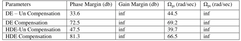
Tab.2: Specifications of lead compensator
Parameters Phase Margin (db) Gain Margin (db) Ωgc (rad/sec) Ωpc (rad/sec)
DE – Un Compensation 33.6 inf 44.5 inf DE Compensation 72.5 inf 69.2 inf HDE-Un Compensation 47.5 inf 39.7 inf HDE Compensation 81.3 inf 66.5 inf
Table shows the specifications of lead compensator by frequency domain technique bode plot. From the above values phase margin greatly improved with compensation over without compensation for both DE and HDE controller tuning techniques. Hence the design of lead compensator for CRPID with HDE optimization technique improves the relative stability of the system.
VI. CONCLUSION
It has been demonstrated that the tuning of PID and CRPID controllers using Hybrid Differential Evolution technique for motor position servo systems is highly effective over Differential Evolution. From simulation results CRPID is more effective than PID controller in all performance aspects and the relative stability of the resultant closed loop system has been greatly improved.
REFERENCES
[1] Guomin Li and Kai Ming Tsang,“Concurrent Relay-PID control Motor Position Servo Systems”: International Journal of Control, Automation and Systems, Vol. 5, no 3, pp. 234-242, june 2007.
[2] Bhawna Tandon, “Genetic Algorithm Based Parameter Tuning of PID Controller for Composition Control System”:International Journal of Engineering Science and Technology, Vol. 3, No.8,Aug,2011.
[3] R.Storn and K.price, “Differential Evolution - A Simple and Efficient Adaptive Scheme for Global Optimization over Continuous Spaces”: Technical report TR-95-012, March 1995,ftp.ICSI.Berkeley.edu/pub/techreports/1995/tr-95-012.ps.Z.
[4] R.Storn and K. Price, “Minimizing the Real Functions of the ICEC’96 contest by Differential Evolution”, proc. Of IEEE Int. Conf. On Evolutionary Computation, Nagoya, Japan 1996.
[5] Lampinen and I. Zelinka, “On stagnation of the differential evolution algorithm,” in: Pavel Ošmera, (ed.) Proc. of MENDEL 2000, 6th International Mendel Conference on Soft Computing, pp. 76 – 83, June 7–9.2000, Brno, Czech Republic.
[7] K .Lakshmi Sowjanya and Dr.L.Ravi Srinivas “Tuning of PID Controller using Hybrid Differential Evolution”, IJAR in Electrical Electronics and instrumentation Engineering , Vol.3, Issue 12, December 2014.
[8] G. Li, “Robust Control Strategies for Motor Servo Systems,” Ph.D. Thesis, The Hong Kong Polytechnic University, Hong Kong, 1999. [9] K. M. Tsang and G. Li, “Robust nonlinear nominal model following control to overcome deadzone nonlinearities,” IEEE Trans. Ind. Electron,
vol. 48, pp. 177-184, 2001.