Article
On some properties of the Glacial Isostatic
Adjustment fingerprints
Giorgio Spada1,‡* 0000-0001-7615-4709 and Daniele Melini2,‡
1 Dipartimento di Scienze Pure e Applicate (DiSPeA), Sezione di Fisica, Università degli Studi di Urbino
“Carlo Bo”, I-61029 Urbino, Italy; Email:[email protected]
2 Istituto Nazionale di Geofisica e Vulcanologia (INGV), Via di Vigna Murata 605, I-00143 Rome, Italy;
Email:[email protected]
* Correspondence: [email protected] ‡ These authors contributed equally to this work.
1
2
3
4
5
6
7
8
9
10
11
12
13
14
15
16
Abstract: Alongwithdensityandmassvariationsoftheoceansdrivenbyglobalwarming,Glacial Isostatic Adjustment (GIA) in response to the last deglaciation stillcontributes significantlyto
present-daysea-levelchange.Indeed,inordertorevealtheimpactsofclimatechange,longterm
observationsattidegaugesandrecentabsolutealtimetrydataneedto bedecontaminated from
theeffectsofGIA.Thisisnowrealizedbymeansofglobalmodelsconstrainedbytheobserved
evolutionofthepaleo-shorelinessincetheLastGlacialMaximum,whichaccountforthecomplex
interactionsbetweenthesolidEarth,thecryosphereandtheoceans. Intherecentliterature,past
andpresent-dayeffectsofGIAareoftenexpressedintermsoffingerprintsdescribingthespatial variationsofseveralgeodeticquantitieslikecrustaldeformation,theharmoniccomponentsofthe
Earth’s gravityfield,relativeandabsoluteseal evel.H owever,sinceitisdrivenbythesluggish
readjustmentoccurringwithintheviscousmantle,GIAshalltaintthepatternofsea-levelvariability
also during the forthcomingcenturies. Theshapes of the GIAfingerprintsr eflectinextricable
deformational,gravitational,androtationalinteractionsoccurringwithintheEarthsystem.Using
up-to-datenumericalmodelingtools,ourpurposeistorevisitandtoexploresomeofthephysical
andgeometricalfeaturesofthefingerprints,theirsymmetriesandintercorrelations,alsoillustrating
howtheystemfromthefundamentalequationthatgovernsGIA,i.e.,theSeaLevelEquation.
Keywords: GlacialIsostaticAdjustment;SeaLevelChange;FingerprintsofPastIceMelting
17
1. Introduction
18
To introduce Glacial Isostatic Adjustment (GIA), it is convenient to define areference statein which
19
the solid Earth, the ice sheets and the oceans are in an equilibrium configuration, sketched in Figure1a, F1a
20
and to compare it to a perturbed state. This approach was originally proposed by Farrell and Clark [1],
21
hereafter referred to as FC76, in their seminal work where the Sea Level Equation (SLE) was introduced
22
first. The reference configuration can be chosen arbitrarily, but for our discussion it is convenient to
23
refer to the Last Glacial Maximum (LGM,∼21, 000 years ago). The load acting on the Earth’s surface in
24
the reference state (i.e.,the mass per unit area) isL0(ω)andI0(ω)is the ice thickness, withω= (θ,λ)
25
whereθis colatitude andλis longitude. The SLE has the purpose of predicting how sea level shall
26
change at an arbitrary locationω, when the configuration of the system portrayed in Figure1a evolves
27
in anew stateshown in Figure1b at timet≥t0, in which the surface load and the ice thickness are F1b
28
L(ω,t)andI(ω,t), respectively. Despite the global variations observed in the new state,i)the mass of
29
the system (ice+oceans+solid Earth) must be conserved, andii)the new sea surface must remain an
30
equipotential; ultimately, these are the two fundamental principles that the SLE makes manifest.
31
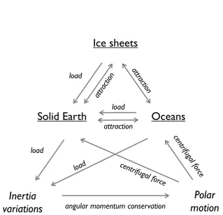
The interactions responsible for the changes observed in the new state are qualitatively sketched
32
in the diagram of Figure2, freely modified from Clarket al.[2]. Since the interactions are operating F2
33
simultaneously and at all spatial scales, their contributions cannot be easily disentangled, which makes
34
the interpretation of the GIA effects on sea level particularly challenging. In the top part, the figure
35
is showing the three fundamental elements of the SLE,i.e.,the ice sheets, the solid Earth, and the
36
oceans [3]. As indicated by the arrows, these elements are interacting by two mechanisms:i)surface
37
loading andii)mutual gravitational attraction. The waxing and waning ice sheets exert a load at the
38
surface of the solid Earth (ice loading, related to glacio-isostasy), but the mass variation of the oceans is
39
also loading the Earth, acting on the seafloor (water loading, associated to hydro-isostasy). These two
40
non-uniform loads are tightly interconnected, since the mass conservation of the system (water+ice)
41
imposes that, on average, the load variation vanishes across the Earth’s surface. Due to the mantle
42
imperfect elasticity, the past loads also induce delayed and still persistent effects that are manifest as a
43
global state of isostatic disequilibrium. Furthermore, the equipotential surfaces of the Earth’s gravity
44
field are twisted by the mass redistributed over the Earth surface and in the oceans, causing variations
45
of the geoid. The three elements that enter into the SLE are all affected by gravitational attraction. In
46
particular, the sea surface is warped by the attraction of the continental ice sheets, but at the same
47
time the geoid variations caused by the solid Earth deformation modify the shape of the oceans. The
48
bottom part of Figure2considers further interactions driven by the Earth’s irregular rotation. Inertia
49
perturbations, associated to long wavelength deformations and sea-level variations of harmonic degree
50
l =2, drive excursions of the rotation axis in order to conserve the Earth’s angular momentum [4].
51
The consequent variation of the centrifugal potential alters, in turn, both the solid Earth and the sea
52
surface and (rotational feedbackon sea level, see Peltier [5]).
53
Theinextricably related interactionsfirst acknowledged by Clarket al.[2] and illustrated in Figure2
54
are responsible for the regional imprints of GIA. As first noted by Woodward [6] and later discussed
55
by Daly [7], Walcott [8] and Farrell and Clark [1], the sea-level variations associated with glacial
isostasy depart significantly from the spatially uniform pattern that we would observe for a rigid,
57
non-gravitating and non-rotating Earth (i.e., ignoring the interactions). Often, in the geological
58
literature the spatially uniform sea-level change is referred to aseustatic, a word attributed to Suess
59
[9]; eustatic variations only depend on the history of the past grounded ice volume [10]. Presently,
60
the termbarystaticis preferred [11]. The interactions are responsible for a global pattern of relative
61
sea level (RSL) variations during the melting of the late-Pleistocene ice sheets, which Clarket al.[2]
62
have characterized by defining sixRSL zones, labelled fromItoV I(see their Figure 5); within each
63
zone, the sea-level signatures are similar to one another. The RSL zones encompass the glaciated
64
areas (zoneI), the region of the collapsing fore-bulge (I I), the time-dependent emergence (I I I) and the
65
oceanic submergence zone (IV), the oceanic emergence region (V), and the continental shorelines (V I).
66
Subsequently, Mitrovica and Milne [12] have studied the nature of the RSL zones in connection with
67
the various terms of the SLE, describing the physical mechanisms responsible for their establishment
68
and unveiling the processes ofcontinental leveringandocean siphoning. Following the above studies,
69
the spatial variability in sea level associated with GIA has been widely investigated with the aim of
70
reconstructing the history of deglaciation since the LGM [seee.g.,13–15]. On a more limited spatial
71
scale, the concept of RSL zone has also been useful to interpret the Holocene sea-level variations across
72
the Mediterranean Sea [16,17].
73
The study of paleo-shorelines has allowed to define the broad features of the pattern of RSL zones
74
since the LGM (see,e.g.,Lambeck and Chappell [18]). However, the present-day trends of sea level
75
detected at tide gauges or by satellite altimetry should be certainly also affected by contemporary
76
variations in the state of the cryosphere driven by global warming. In this context, the question has not
77
been addressed until the work of Plag and Jüettner [19], who have first coined the term offingerprint
78
(function). . . The elastic response of the Earth to present-day changes in the cryosphere can be expected to
79
produce a similar fingerprint, which should be present in the tide gauge data. Based on these fingerprints, tide
80
gauge trends, in principle, can be inverted for ice load changes[19]. However, after having analyzed the
81
relative sea-level trend for some long tide gauge time series, Douglas [20] concluded thatunambiguous
82
evidence for fingerprints of glacial melting was not found, most likely due to the presence of other signals
83
present in sea-level records that cannot easily be distinguished. Recently, Spada and Galassi [21] have
84
quantitatively compared the harmonic power spectrum of contemporary sea-level change to that of
85
GIA, including the contribution due to the disintegration of the past ice sheets and that associated to
86
present deglaciation. They have shown that thepowerof GIA from past ice melting is comparatively
87
modest at all harmonic degrees, with the possible exception of harmonic degreel=2, and it cannot
88
emerge from the steric component that dominates current sea-level rise [22]. Notwithstanding the
89
difficulty of visualization, the concept of sea-level fingerprint has undoubtedly gained an important
90
role in the interpretation of the trends of contemporary [23–27] and future sea-level rise [28–30].
In this work, we aim at exploring and reviewing the properties and the symmetries of the GIA
92
fingerprints presently associated with the melting of past ice sheets, as well as the intercorrelations
93
among them. Much of what we present in this paper can be also applied to the fingerprints of present
94
ice melting, which obey the SLE as well; these have been discussed in various places, seee.g.,[31]
95
and references therein. Although we are aware that uncertainties on the Earth’s viscosity profile
96
and the chronology of deglaciation affect significantly the pattern and the amplitude of the GIA
97
fingerprints [32], here for simplicity we shall only consider a specific GIA model, leaving an error
98
analysis to future work, along the lines of Melini and Spada [32]. The paper is organized as follows. In
99
Section2we review the theory behind the SLE. In Section3we briefly present the GIA model used and
100
the numerical approach adopted. In Section4we illustrate some of the properties of the present-day
101
GIA fingerprints associated with the melting of the past ice sheets, which in Section5are exploited to
102
interpret the global uplift pattern of continents currently detected by GPS data. Our conclusions are
103
drawn in Section6.
104
2. Theory
105
Here we briefly introduce the essentials of the SLE theory, necessary to illustrate the geometry of
106
the GIA fingerprints in Section4below. The reader is referred to Spada and Melini [33] (hereinafter
107
SM19) and to its supplement for a more detailed and self-contained presentation1. We note that the
108
SLE theory does not account for tectonic deformations nor for variations in the temperature or salinity
109
of the ocean water, which we do not consider in our analysis.
110
In the reference state considered in Figure1a,sea levelis defined by the difference
111
B0(ω) =r0ss−rse0, (1)
112
whereω= (θ,λ)are the coordinates of a given point on the Earth’s surface,r0ss(ω)andrse0(ω)are the
113
radii of the (equipotential) sea surface and of the solid Earth in a geocentric reference frame with origin
114
in the whole-Earth center of mass, respectively. As shown in Figure1a,B0would be directly measured
115
by a stick meter,i.e.,atide gauge, placed atω. Assuming that the horizontal displacement of the
116
stick-meter has been negligible in comparison to vertical displacement, in the new state, sea level is
117
B(ω,t) =rss−rse, (2)
118
1 The paper SM19 and its supplement are submitted to Geoscientific Model Development (GMD), the interactive open-access
journal of the European Geosciences Union athttps://www.geosci-model-dev-discuss.net/gmd-2019-183/. The open-source
whererss(ω,t)andrse(ω,t)denote the new radius of the equipotential sea surface and of the solid
119
surface of the Earth, respectively. Note thattopographyis related to sea level through
120
T(ω,t) =−B. (3)
121
Combining (2) with (1),relative sea-level change
122
S(ω,t) =B−B0 (4)
123
can be also expressed as
124
S(ω,t) =N − U, (5)
125
where
126
N(ω,t) =rss−r0ss (6)
127
is thesea surfacevariation, orabsolute sea-level change, and
128
U(ω,t) =rse−r0se (7)
129
is thevertical displacementof the Earth’s surface. Eq. (5) represents the most basic form of the SLE. We
130
note that, being defined as a double difference, relative sea-level changeS(ω,t)is not dependent upon
131
the choice of the origin of the reference frame,i.e.,it is an absolute quantity. QuantitiesN(ω,t)and
132
U(ω,t), however, depend on the choice of the origin.
133
The sea surface variation N(ω,t) is tightly associated to the variation of the geoid height.
134
However, as remarked by FC76,N(ω,t)is notthevariation of the geoid. . . on a rigid earth model,
135
there is no distinction between changes in geoid radius and changes in sea level, but it is important to realize
136
the difference between these quantities for deformable Earth models[1]. A further problem arises from the
137
fact that, in the new state, the volume of the oceans is varied to compensate the mass lost or gained by
138
the continental ice sheets. Indeed, as pointed by Tamisiea [34], some confusion arose recently about
139
the definition ofN(ω,t), which sometimes is still used as a synonymous of geoid height variation;
140
the confusion is attributed to often inconsistent terminology between various disciplines. FC76 have
141
shown that the sea surface height variation is
142
N(ω,t) =G+c, (8)
where
144
G(ω,t) = Φ
g, (9)
145
is thevariation of the geoidradius relative to the reference state, Φ(ω,t)is the variation of the total
146
gravity potential of the Earth system, taking both surface loading and rotational contributions into
147
account,gis the reference surface gravity acceleration andcis a yet undetermined spatially invariant
148
term notorious within the GIA community as theFC76 c-constant. In the following, Eq. (8) shall be
149
referred to asFC76 formula. Thus, using Eq. (8) in (5), the SLE reads
150
S(ω,t) =R+c, (10)
151
where we have defined thesea-level response functionby the difference
152
R(ω,t) =G − U. (11)
153
It is now convenient to average both sides of Eq. (10) over the oceans, where the ocean-average of
154
any functionF(ω,t)is defined, at timet, as
155
<F(ω,t)>o(t)≡ 1 Ao
Z
oF(ω,t)dA, (12)
156
whereR
odenotes the integral over the time-dependent surface of the oceans,Aois their area at time
157
t,dA =a2sinθdθdλis the element of area over the surface of the sphere, andathe average Earth’s
158
radius. We recall that the surface of the oceans is the region whereO=1, whereOis theocean function
159
(OF) is defined as
160
O(ω,t) =
1 ifT+ ρ i
ρwI<0
0 ifT+ ρ i
ρwI≥0,
(13)
161
whereρiandρware the densities of ice and water, respectively. ForO=1, the ocean is ice-free, or there
162
is floating ice; forO= 0, the ice is grounded either below or above sea level, or the land is ice-free.
163
Using acontinent functiondefined asC(ω,t) =1−Ois sometimes useful. Since<c>o≡c, solving
164
Eq. (10) with respect to the FC76 constant gives
165
c(t) =Save−<R>o, (14)
where we have definedSave≡<S >o. Hence, using Eq. (14) into (10), the SLE is further transformed
167
into
168
S(ω,t) =R+Save−<R>o . (15)
169
The response functionR(ω,t)embodies all the interactions qualitatively described in Figure2;
170
following SM19, we split it into a contribution due to surface loadsandgravitational attraction (labeled
171
bysur) and one due to rotational effects (rot), with
172
R(ω,t) =Rsur+Rrot, (16)
173
whereRsur(ω,t) =Gsur− UsurandRrot(ω,t) =Grot− Urot. According to Farrell [35],Rsuris given
174
by a 3-D spatio-temporal convolution that involves thesurface Green’s function for sea levelΓsand the
175
surface load variationL=L−L0, with
176
Rsur(ω,t)≡Γs⊗ L, (17)
177
while following Milne and Mitrovica [36],Rrotcan expressed as a 1-D time convolution between
178
therotation Green’s function for sea levelΥsl and thecentrifugal potential variation, with
179
Rrot
lm(t) =Υsl∗Λlm, (18)
180
where (l,m) are the spherical harmonic degree and order, respectively (l=0, 1, 2, . . . ,lmax;|m| ≤l).
181
Han and Wahr [37] and Milne and Mitrovica [36], however, have shown thatΛ(γ,t)is essentially a
182
spherical harmonic function of degree and order(l,m) = (2,±1). The Green’s functionsΓsandΥs l are
183
expressed by particular combinations ofloading Love numbersandtidal Love numbers, respectively. It is
184
important to note that the harmonic coefficients ofRsur(ω,t),i.e.,Rsur
lm(t), depend linearly from those
185
of the surface load variationLlm(t)(see supplement of SM19 for details).
186
An explicit expression forSavein Eq. (15) is obtained applying the mass conservation principle
187
that according to SM19 can be stated in various equivalent ways. Here it is convenient to use the form
188
<L>e(t) =0, (19)
where the average over the whole Earth’s surface is defined, in analogy with Eq. (12), as< · · ·>e
190
(t)≡(1/Ae)∫e(· · ·)dA. We refer to mass conserving loads that obey Eq. (19) asphysically plausible
191
loads. As shown in SM19, condition (19) is equivalent to
192
L00(t) =0, (20)
193
whereL00(t)is the spherical harmonic component of the surface load for degree and order(l,m) =
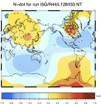
194
(0, 0). Using the result
195
L(ω,t) =ρiIC+ρwBO, (21)
196
(SM19) and some algebra, from the constraint of mass conservation we obtain
197
Save(t) =Sequ+So f u, (22)
198
whereSequ(equivalent sea-level change) is defined as
199
Sequ(t) =− µ
ρwAo, (23)
200
withµ(t) =ρi∫e(IC−I0C0)dAdenoting the time variation of the grounded ice mass, and term
201
So f u(t) = 1 Ao
Z
eT0(O−O0)dA, (24)
202
is associated with ocean function variations, whereT0andO0are the initial topography and the initial
203
OF, respectively. We note that in the fixed-shorelines approximation of FC76, the OF is constant,
204
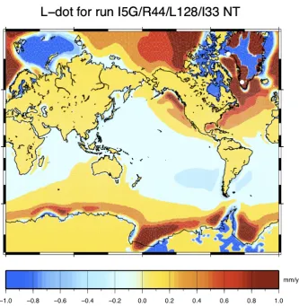
withO=O0 =OpwhereOpis the present OF. Hence, in this approximationSo f u =0, andSequis
205
equivalent to what in the geological literature is often calledeustatic[9] sea-level change
206
Seus(t) =− µ
ρwAop, (25)
207
whereAop=∫
eOpdAis the present-day area of the oceans.
208
The SLE (15), complemented by Eqs. (16-18) and (22) constitutes a 3-D non-linear integral equation
209
in the unknownS(θ,λ,t), somewhat similar to a 1-D non-homogeneous Fredholm equation of the
210
second kind [seee.g.,38]. Assuming fixed shorelines, as in FC76, would reduce the SLE to a linear
211
equation [31]. The integral, or implicit, nature of the SLE becomes apparent when it is recognized that
212
the response functionRfunctionally depends, throughGandU, uponS itself (see SM19). In modern
213
approaches to GIA, the SLE is solved recursively in the spectral domain, adopting thepseudo-spectral
214
method [39,40].
In the general case given by Eq. (15), no analytical solutions exist for the SLE. However, a
216
closed-form solution can be found in the eustatic approximation, expressed by (25), valid in the very
217
special case of a rigid Earth in which the gravitational attraction between the three components of
218
the SLE is neglected (see Fig.2). Another analytical solution is found assuming a rigid Earth and
219
uniform oceans but allowing for the gravitational interaction between the ice sheets and the oceans,
220
i.e.,neglecting the self-attraction of oceans. This solution, often referred to asWoodward solution[6], has
221
been discussed in detail bye.g.,Spada [31]. Although oversimplified, it has the merit of demostrating
222
the important role of gravitational attraction in shaping the sea surface, with a sea-level change
223
departing from the spatially uniform eustatic solution both nearby the melting ice sheets and in their
224
far field.
225
3. Methods
226
Spada and Melini [33] have recently released a general open-source Fortran program called
227
SELEN4(SELEN version 4.0) that solves the SLE in its full form; this shall be employed in next sections
228
to study the geometry of the GIA fingerprints associated with the melting of past ice sheets. SELEN4is
229
the current stage of the evolution of programSELENwhich was originally published in 2007 by Spada
230
and Stocchi [41] based upon the theory detailed in Spada and Stocchi [42].
231
SELEN4implements the pseudo-spectral method of Mitrovica and Peltier [39] and Mitrovica
232
and Milne [40]. In SELEN4, all the variables have a piecewise constant time evolution. In space,
233
the discretization is performed adopting the equal-area icosahedron-based spherical geodesic grid
234
designed by Tegmark [43], whose density is controlled by the resolution parameter R. In our
235
computations, we have setR = 44, corresponding toP = 40R(R−1) +12 = 75, 692 pixels over
236
the sphere, each having a radius of∼46 km. In this way, the number of cells is comparable to that
237
of a traditional 1◦×1◦spherical grid,i.e.,64, 800. The spherical harmonic expansions required in the
238
framework of the pseudo-spectral approach are truncated at degreelmax =128 and the coefficients
239
are evaluated taking advantage of the quadrature rule for the Tegmark grid [43]. According to SM19,
240
the chosen combination (R,lmax) ensures a sufficient precision without being computationally too
241
demanding.
242
In SELEN4, we have implemented the GIA model ICE-5G of Peltier [44]. The ice thickness has
243
been discretised on the Tegmark grid and reduced, at a given pixel, to a uniform sequence of identical
244
time steps with a length of 500 years. The LGM is at 21 ka, and prior to that isostatic equilibrium is
245
assumed. Since the LGM, ICE-5G releases a total equivalent sea level
246
ESL=ρi/ρw ∆Vi/Aop
=127.3 m, (26)
where we have assumedρi=931.0 andρw=1000.0 kg m−3, and∆Viis the ice volume variation since
248
the LGM. We combine the ICE-5G deglaciation history with a three-layer volume-averaged version of
249
the VM2 multi-stratified rheological profile [44]. The Maxwell viscosities areη=2.7, 0.5 and 0.5 in
250
units of 1021Pa·s in the lower mantle, transition zone and shallow upper mantle, respectively. The
251
core is fluid inviscid and the elastic lithosphere is 90 km thick. A PREM-averaged [45] density and
252
rigidity profile has been adopted, using a 9-layer structure. Loading and tidal Love numbers have
253
been computed using programTABOO[46] in a multi-precision environment [47], and expressed in a
254
geocentric reference frame with origin in the center of mass of the whole Earth, including the solid and
255
the fluid portions.
256
The SLE has been solved iteratively [48] adopting three “external” iterations to progressively
257
refine the OF and the paleo-topography and, for each of them, performing three “internal” iterations to
258
solve forS(ω,t), for a given an approximation of topography. According to SM19 and to independent
259
results by Milne and Mitrovica [36], these choices ensure sufficiently precise results. The present-day
260
relief, obtained by a pixelization of the ice-free version of model ETOPO1 [49,50], has been imposed
261
as afinalcondition. The present-day ice distribution is given by the last step of ICE-5G. Finally, to
262
model the effects of polar motion on sea-level change, we have employed therevised rotation theoryby
263
Mitrovicaet al.[51] and Mitrovica and Wahr [52]. Some runs, however, have been performed adopting
264
thetraditional rotation theory(seee.g.,Spadaet al.[46] and references therein) or totally neglecting the
265
effects of Earth rotation.
266
4. Some properties of the GIA fingerprints
267
In the next subsections we provide an overview of the properties of the GIA fingerprints for
268
the present-day trends ofi)relative sea-level ( ˙S),ii)vertical displacement ( ˙U),iii)geoid height ( ˙G),
269
iv)absolute sea level ( ˙N), andv)surface load ( ˙L), respectively. The list is by no means exhaustive,
270
and it should be also extended to other quantities associated with GIA, as for example the horizontal
271
displacement and the free air gravity anomalies. Future releases of SELEN4shall include modules for
272
these and possibly other GIA fingerprints. Note that since the equipotential surfaces of the gravity
273
field and the solid surface of the Earth are defined at all grid points, the map of ˙Sand of all the other
274
fingerprints considered in the following are also extended across the continents. As GIA evolves over
275
millennia, the geometry of the fingerprints would not change appreciably on time scales of a few
276
centuries [53].
277
4.1. Relative sea-level change
278
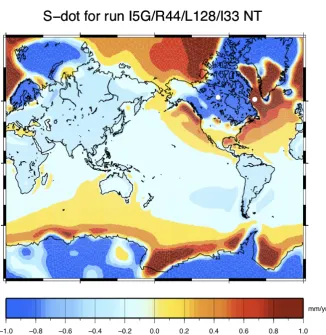
Figure3shows the GIA fingerprint ˙S(ω),i.e.,the rate of present-day relative sea-level change. F3
279
Assuming that GIA from the melting of past ice sheets is the unique cause of contemporary
sea-level change, the rates shown in Figure3would be directly observable as constant secular trends at
281
tide gauges [seee.g.,31]. The ˙Sfingerprint shows the major features and patterns of regional variability
282
already described by Mitrovica and Milne [12],i.e.,the strong relative sea-level fall associated with post
283
glacial rebound across the polar regions that where once covered by thick ice sheets and corresponding
284
toRSL zone Iof Clarket al.[2], the sea-level rise across the ring-shaped collapsing lateral fore-bulges
285
(zoneI I), and the region of broad sea-level fall associated with equatorial ocean syphoning (zoneV).
286
The offshore sea-level rise clearly evident in the equatorial regions in the GIA maps of Mitrovica and
287
Milne [12] and Melini and Spada [32], and linked to continental levering (zoneV I), does not stand out
288
clearly in Figure3, except perhaps along the coasts of central Africa and Australia. In part, this could
289
be due to the different deglaciation chronology and rheology adopted in [12,32], corresponding to
290
model ICE-3G (VM1) of Tushingham and Peltier [54]. However, by a further SELEN4run, in which we
291
have still adopted model ICE-5G (VM2) but we have ignored rotational effects as done in [12,32], we
292
have ascertained that the localised offshore sea-level rise is clearly detectable. Thus, we conclude that
293
in Figure3this feature is almost completely blurred by the long-wavelength effects of Earth rotation.
294
The rotational feedback on sea level is responsible for the southern hemisphere swaths of sea-level rise
295
and fall around Oceania and South America, respectively. In the northern hemisphere, these effects are
296
less evident, due to the dominating contribution of glacial unloading and of the peripheral subsidence.
297
A crude but useful way to simplify the evident geometrical complexity of GIA fingerprint in
298
Figure3is to evaluate its spatial average (all spatial averages of the GIA fingerprints discussed in the
299
following are collected in Table1). For the ocean-average of ˙S(ω), given by<S˙ >o, the SLE theory T1
300
provides an explicit formula, which stems from the constraint of mass conservation. It can be obtained
301
by computing the time-derivative of Eq. (22), also taking (23) and (24) into consideration. However, a
302
numerical evaluation on the grid is more convenient, which according to our computations gives the
303
small value
304
<S˙>o=−0.05 mm yr−1, (27)
305
where conventionally we shall use the termsmallto indicate all GIA rates<0.1 mm yr−1in modulus.
306
A three-fold larger but coherent value, with<S˙ >o=−0.14 mm yr−1, was computed by Spada [31],
307
who however adopted the traditional rotation theory. By inspection of Eqs. (23-24), the small value of
308
<S˙ >omay reflect minor variations of the OF associated to changes in the areaAo(t)of the ocean
309
basins, tiny values of the rate of change of the grounded ice massµ(t), or both. Since in model ICE-5G
310
(VM2) the mass distribution over Greenland has seen small but significant variations during the last
311
≈6, 000 years that continue to present [55], the average<S˙>oeffectively reflects both contributions.
312
However, if we had employed a GIA model that assumes no ice sheets fluctuations during the last few
kyrs, like ICE-3G (VM1) [54,56] or ICE-6G (VM5a) [57], also imposing fixed shorelines as in FC76, we
314
would have obtainedexactly
315
<S˙>o
FC76=0 mm yr−1, (28)
316
as a direct consequence of mass conservation. In fact, this result would be achieved regardless the
317
rheological profile chosen. We note that the SLE theory tells nothing about the whole-Earth-surface
318
average<S˙>e, which however according to our computations in Table1is not small.
319
4.2. Vertical displacement
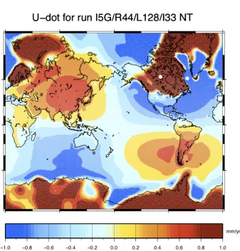
320
In Figure4we show the GIA fingerprint ˙U(ω), which represents the present-day rate of change of F4
321
the vertical displacement that would be observed, at a given location, by an earthbound GPS receiver
322
[58–61]. By a visual inspection, it is apparent that most of the features of this map are anti-correlated
323
with those shown by fingerprint ˙S(ω)in Figure3. In particular, this occurs in previously glaciated
324
areas and in their surroundings, where a relative sea-level rise is accompanied by subsidence, and
325
viceversa. However, we note that apparently paradoxical conditions as having a relative sea-level rise
326
in uplifting regions, or a relative sea-level fall in subsiding regions, are not forbiddena prioriby the
327
SLE (see Eq.5). These conditions may well occur where the rate of absolute change ˙N(ω), shown in
328
Figure6below, attains positive and negative values, respectively.
329
The anti-correlation between ˙U(ω)and ˙S(ω)is not so evident across the equatorial basins, where
330
the ˙U(ω)fingerprint shows a clear sectorial symmetry of harmonic degree and order(l,m) = (2,±1),
331
which manifests the long-wavelength effects of Earth rotation. By a comparison with Figure3, it
332
turns out that such symmetry is definitively more compelling for ˙U(ω)than for ˙S(ω). In the northern
333
hemisphere, the rotation-induced subsidence across North America counteracts the uplift associated
334
with the melting of Laurentide ice sheet, but it intensifies the subsidence across the peripheral
335
fore-bulges. Conversely, in Asia the effects associated to Earth rotation are clearly enhancing the
336
vigor of the uplift induced by continental levering [12]. Interestingly, Figure4reveals that a number
337
of GIA-associated processes coherently concur to the uplift in Patagonia, which is caused by local
338
effects due to un-loading of the former Patagonian ice sheet included in model ICE-5G (VM2), by the
339
contribution of continental levering and by the effect from Earth rotation. The unloading associated
340
with the melting of contemporary glaciers and ice caps [62,63], which however is not taken into account
341
in our modeling, would act is the same direction.
As we have done for ˙S(ω)above, it is useful now to consider spatial averages of the fingerprint
343
in Figure4. To a very high precision (see Table1), the whole-Earth average of ˙U(ω)is numerically
344
found to be
345
<U˙ >e=0.00 mm yr−1, (29)
346
a property of the ˙U(ω)fingerprint that, once again, is explained in terms of the principle of mass
347
conservation. Since we have assumed aplausiblesurface load, mass conservation is ensured by Eq. (20).
348
From Eq. (17), this implies a vanishingRsur(ω,t)at harmonic degree and order(l,m) = (0, 0), from
349
which the fundamental property (29) of the ˙U(ω)fingerprint follows immediately. We note that this
350
characteristic is totally unaffected by the choice of the GIA model and, in particular, from the Earth
351
rheological profile assumed. It also holds true when, in GIA modeling, one neglects rotational effects
352
and the horizontal migration of the shorelines, as done for example in the FC76 formulation (this is
353
confirmed by the results in Table1). Furthermore, as long as the mass conservation constraint is not
354
violated, it is also valid for the ˙U(ω)fingerprint associated to the present melting of continental ice
355
sheets, for which viscous rheological effects can be neglected [31,34].
356
We finally note that the SLE theory tells nothing about the GIA-induced average rate of subsidence
357
of the ocean floors< U˙ >o, which however according to our computations reported in Table1, is
358
found not to be small. This would support the idea of a significant influence of climate variations on
359
the isostatic equilibrium of the sea floor topography [64,65]. The negative value of<U˙ >ois easily
360
justified by the dominance, in Figure4, of blue swaths across the oceans caused by the effect of water
361
loading. Conversely, by the argument of mass conservation, we expect a not small and positive value
362
<U˙ >c, where superscriptcdenotes the average over the continents. We shall return on this issue in
363
Section5below.
364
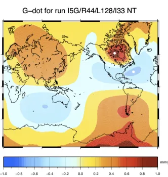
4.3. Geoid height and absolute sea-level change
365
In Figure5we show the map of the GIA fingerprint for ˙G(ω). According to Eq. (9), this quantity F5
366
represents the present-day rate of change of the geoid height. It appears that ˙G(ω)is characterized by
367
a well developed lobed symmetry with(l,m) = (2,±1)and, with respect to ˙S(ω)and ˙U(ω), by an
368
overall smoother resemblance. The cause is to be found in the different spectral content of theh(t)and
369
k(t)loading Love numbers that contribute to ˙U(ω)and ˙G(ω), respectively; see SM19 for details. The
370
pattern associated to Earth rotation is so strong that the regional effects from glacial unloading are
371
only just visible in the polar regions of both hemispheres. To suitably interpret the(l,m) = (2,±1)
372
symmetry, it is worth to note that according to our computations, the GIA-induced polar motion
373
presently occurs at a rate of∼1.3 deg/Myr (roughly corresponding to 10 cm/yr on the Earth’s surface)
374
along the meridian∼ 78◦W (roughly, towards the Hudson Bay). Such rate and direction of polar
drift match well the astronomical observations in the course of last century (seee.g.,Lambeck [4]).
376
Performing a further run of SELEN4in which we have adopted thetraditional rotation theory(seee.g.,
377
Spadaet al.[46]), we have verified that the(l,m) = (2,±1)pattern of ˙G(ω)would be indeed much
378
stronger, with a three-fold rate of polar drift of∼3.5 deg/Myr in the same direction. The enhanced
379
rate of polar motion implied by the traditional rotation theory compared to the new theory is in full
380
agreement with the analysis of Mitrovicaet al.[51] and Mitrovica and Wahr [52].
381
Based upon the same argument we have used for ˙U(ω)above (i.e.,mass conservation ensured by
382
plausible surface loads), the fundamental property of the ˙G(ω)fingerprint can be similarly expressed
383
by
384
<G˙ >e=0.00 mm yr−1, (30)
385
which we have verified numerically to be valid to a very high precision (see Table1). In consequence
386
of (30), harmonics with(l,m) = (0, 0)are not contributing to ˙G(ω). We further note that condition
387
< G˙ >o≈< U˙ >o, suggested by the results in columna) of Table1, is due to chance and it is not
388
reflecting any particular property of the GIA fingerprints. Indeed, when the traditional rotation theory
389
is adopted or rotation is neglected, as done in columnsb) andc), respectively, or alternative GIA
390
models such as ICE-6G (VM5a) are employed as in SM19, this condition is not met.
391
As shown bye.g.,Melini and Spada [32], the individual harmonic components of ˙G(ω),i.e.,G˙lm,
392
are proportional to the rates of change of the GIA-induced variations of the Stokes coefficients of the
393
Earth’s gravity field, detectable by the Gravity Recovery and Climate Experiment (GRACE); see Wahr
394
et al.[66] for a discussion. In particular,
395
˙
δclm+iδs˙lm=a−1
p
2−δ0m G˙lm∗ , (31)
396
whereδclmandδslmare the variations of the fully normalised cosine and sine Stokes coefficients,
397
i =√−1 is the imaginary unit,ais the reference Earth’s radius,δijis the Kronecker delta, and the
398
asterisk denotes complex conjugation. We also note that since we are solving the SLE in a geocentric
399
reference frame with origin in the whole-Earth center of mass, a further property of the field ˙G(ω)
400
is that of not having contributions from the harmonics of degree and order(l,m) = (1, 0) and
401
(l,m) = (1,±1)[67]. Hence, in Eq. (31), only terms with harmonic degreel≥2 appear.
402
The GIA fingerprint for ˙N(ω), shown in Figure6, represents the present-day rate of change of F6
403
the sea surface height (or absolute sea level) that would be observed across the oceans by satellite
404
altimetry [22,31], assuming that only GIA is contributing to contemporary sea-level change. It is
405
worth to recall that, regardless the rotation theory adopted in GIA modeling, the ˙N(ω)fingerprint
406
is not independent upon ˙S(ω)and ˙U(ω), since from the basic form of the SLE (see Eq.5), we have
˙
N(ω) =S˙(ω) +U˙(ω). Actually, in view of the relatively small range of values spanned by ˙N(ω),
408
which never exceeds the value of 1 mm yr−1in modulus, the approximation of the SLE ˙S(ω)≈ −U˙(ω)
409
is inviting, but it would be an oversimplification. We further note that only in the idealized case of an
410
un-deformable Earth, with ˙U(ω) =0, absolute and relative sea-level variations would coincide, with
411
˙
S(ω) =N˙(ω).
412
By the FC76 formula, it turns out that ˙N(ω)is strongly associated to the rate of geoid change,
413
since it simply differs from ˙G(ω)by the spatially invariant quantity ˙c, where ˙cis the time-derivative of
414
the FC76 constant. In consequence of the FC76 formula, the whole-Earth surface average of ˙N(ω)is
415
<N˙ >e=c˙=−0.22 mm yr−1, (32)
416
which turns out to be an appealingly simple definition of ˙c. Using the gridded data shown in Figure6,
417
we numerically obtain a not small ocean average
418
<N˙ >o=−0.27 mm yr−1, (33)
419
a (GIA model dependent) value closely matching<N˙ >o=−0.3 mm yr−1, often adopted as arule
420
of thumbto correct the altimetric absolute sea-level trend for the effects of past GIA [see31,34, and
421
references therein]. Since during the altimetry era (1992-today) the rate of global mean sea-level rise
422
has well exceeded∼ 3 mm yr−1 [68,69], using the average (33) to perform the GIA correction is
423
certainly justified. However, spatial trends of ˙N(ω)at a regional scale may become important when
424
one considers the effects of present land ice on absolute sea level change, as done by Ponteet al.[70].
425
4.4. Surface load
426
We conclude our overview with a few remarks about the GIA fingerprint for ˙L(ω), the present-day
427
rate of change of the surface load. This quantity, which is shown in Figure7in units of mm yr−1of F7
428
water equivalent, describes the local variations in the distribution of the ice and water. We recall that
429
the load variationL(ω,t)is defined asL−L0, whereL(ω,t)is given by Eq. (21) andL0is the value
430
ofLin the reference state (see Figure1). To interpret the gross features of the map shown Figure7,
431
for one moment it is convenient to assume that the continent functionCand the ocean functionOare
432
constant to the present day values, as it would be implicit in the FC76 formulation of GIA. If this holds
433
true, by evaluating the time-derivative of Eq. (21) at present time we obtain
434
˙
L(ω)'ρiI˙C+ρwSO˙ , (34)
435
whereI = I−I0is the ice thickness variation and we have also used the definition of sea-level change
436
given by Eq. (4). Across the oceans, the existence of the positive correlation between ˙L(ω)and
˙
S(ω)predicted by Eq. (34) is easily recognized comparing the fingerprints in Figures7and3. The
438
strong contribution to ˙L(ω)across Greenland is associated with the current ice variation that ICE-5G
439
(VM2) embodies in this region [44,55]; in all other continental areas the load variation vanishes, in
440
agreement to Eq. (34). A notable exception is West Antarctica, where the negative trend of the load
441
is associated with the significant variations of the ocean function in this region, associated with the
442
still continuing transition between grounded and floating ice. However, this is not accounted for in
443
the FC76 approximation (34), which assumes a constant OF. Lastly, we observe that once integrated
444
over the whole Earth’s surface,L(ω,t)gives the global mass change of the system with respect to the
445
reference state. However, since mass is conserved, consistently with Eq. (19), we have
446
<L˙>e=0.00 mm yr−1, (35)
447
which according to Table1is numerically verified to a very high precision.
448
5. Observing the global GIA fingerprint by vertical GPS rates
449
As an example of application of the fingerprints properties illustrated above, we mention the
450
problem of using directly geodetic observations to quantify the present global pattern of GIA. Recently,
451
using a large global compilation of geodetic GPS rates in conjunction with a Bayesian inference method,
452
Hussonet al.[71] have reconstructed and visualized the long-wavelength signature of GIA on the
453
rate of present day vertical crustal uplift. In principle, once the contributions from short-wavelength
454
tectonic phenomena have been filtered out, the geodetically observed rates across the continents should
455
match those predicted by current GIA models, at least in their global traits and in their spatial averages.
456
One possible way to verify this consistency is to consider the average over the continents of the
457
geodetically determined rate of vertical uplift<U˙ >c(t), where<· · ·>c(t)≡(1/Ac)∫
c(· · ·)dA,
458
Ac(t) = Ae−Ao being the area of the continents. In Hussonet al.[71], the scalar field ˙U has been
459
estimated from GPS vertical rates by a self-adaptive trans-dimensional regression that exploits the
460
properties of the Voronoi tesselation. The pattern of GIA inferred by regression has been found
461
to broadly resemble the one that we would expect by a model like ICE-5G (VM2), provided that
462
components with wavelengths<2, 500 km are removed.
463
Of course, the average<U˙ >ccould be evaluated numerically using the results of Figure4and
464
compared to the value obtained from the pattern of the GPS rates. However, through the SLE, it is
465
straightforward and possibly more meaningful to express< U˙ >cin terms of the ocean-averaged
466
fingerprints<S˙ >oand<N˙ >o that we have already discussed above in view of their particular
467
significance. Here we largely follow Hussonet al.[71] and, since we simply aim at illustrating the
method, we do not consider the modeling uncertainties on the GIA fingerprints. On one hand, taking
469
advantage of Eq. (29), we have
470
1
Ae
Z
e ˙
UdA=0, (36)
471
which by the additivity of the surface average gives
472
1
Ae
Z
c ˙
UdA+
Z
o ˙
UdA
=0 , (37)
473
or, equivalently,
474
Ac
Ae <U˙ > c+Ao
Ae <U˙ >
o=0 , (38)
475
where we have used the definitions of continent and ocean average; hence
476
<U˙ >c=−A o
Ac <U˙ >
o. (39)
477
On the other hand, ocean-averaging both sides of the SLE in the form (5) gives
478
<U˙ >o=<N˙ >o−<S˙>o, (40)
479
which used into (39) yields the average of ˙Uacross the continents
480
<U˙ >c= Ao
Ac <S˙ >
o−<N˙ >o
, (41)
481
which is only expressed in terms of ocean-averaged fingerprints.
482
The exercise above shows that the average vertical uplift across the continents determined by GPS
483
could be estimated,in principle, by ocean-averaging the tide gauge trends and subtracting the ocean
484
averaged altimetry-derived rate of absolute sea-level change. This would hold true regardless the GIA
485
model employed. By approximatingAo≈(7/10)AeandAc≈(3/10)Ae, so thatAo/Ac≈7/3, and
486
using the ocean averages for ICE-5G (VM2) given by Eqs. (27) and (33), we obtain the not small value
487
<U˙ >c≈0.51 mm yr−1, (42)
488
where we note that since in Eq. (41) Husson et al. [71] have used the crude fixed-shorelines
489
approximation that implies< S˙ >o= 0 they have obtained slightly different values for< U˙ >c.
490
Nevertheless, the value of< U˙ >cmatches the rate effectively reconstructed by Hussonet al.[71]
491
(0.64 mm yr−1)reasonably well. This suggests that the trans-dimensional regression method has been
effective in isolating the fingerprint of GIA. As pointed by Hussonet al.[71], the effects of current
493
melting of glaciers and ice caps in response to global warming would not alter substantially result (42).
494
6. Conclusions
495
In this work we have reviewed some aspects of GIA, i.e., the response of the Earth to the
496
disequilibrium caused by the melting of the late-Pleistocene ice sheets. Arguments based upon the
497
physical properties of the SLE have been corroborated by results obtained from up-to-date numerical
498
tools in GIA modeling. Among the processes that concur to present sea-level rise, the special role of
499
GIA has been recognized long ago; in fact, only GIA is affected by the rheology of the Earth and, at
500
the same time, it affects significantly the gravity field and the rotational state of the planet. Although
501
according to current GIA models the deglaciation of the late-Pleistocene ice sheets came to an end
502
thousands of years ago, at present the effects of GIA are still significant and they influence a number of
503
directly observable geophysical and geodetic quantities. Since GIA evolves slowly, its contribution to
504
the instrumental observations will persist also during next centuries although it shall gradually fade
505
away. Model predictions show that the computed patterns or fingerprints of GIA are characterized by
506
an outstanding complexity. In our roundup of the general properties of the GIA fingerprints, we have
507
considered both the geometrical and the physical aspects of such complexity, emphasizing their spatial
508
symmetries and regional character, which we have interpreted qualitatively and quantitatively with
509
the aid of the SLE.
510
The study of the relative sea level fingerprint has revealed that at present the role of GIA is not
511
that of causing an effective, mean global change. Rather, it causes essentially local regional effects
512
which strongly contaminate the tide gauges records but thatalmostwash out when averaged over
513
the present-day oceans, leaving a small contribution reflecting minor variations in the area of the sea
514
floor and possibly current variations of ice thickness, when these are accounted for by the GIA model.
515
The coastal regions are certainly those being most affected by the regional variability of GIA. The
516
pattern of the GIA-induced vertical uplift is extremely variegated but it globally averages out to zero
517
as an effect of mass conservation. Although it is largely anti-correlated to that of relative sea level, it
518
shows more clearly the mark of the rotational effects of GIA, with a symmetry dominated by a very
519
long-wavelength harmonic pattern. By a specific example from the recent literature, we have shown
520
that the basic traits of the GIA fingerprint of vertical displacement can be visualized using data from a
521
large global compilation of geodetic GPS rates. The symmetry imposed by the polar drift of the rotation
522
axis is even more enhanced when one considers the fingerprints of the geoid height variation and of
523
the absolute sea-level change, which only differ by a spatially invariant term. These two last signatures
524
of GIA have presently a particular role in physical geodesy, since they are commonly employed to
purge the trends of the Stokes coefficients of the gravity field and the sea-level altimetric records from
526
the GIA effects.
527
In this study, we have employed only one of the ICE-Xmodels of WR Peltier and collaborators [44].
528
Independently obtained GIA models exist, like those progressively developed at the National
529
Australian University by Kurt Lambeck and colleagues (see Nakada and Lambeck [72], Lambeck
530
et al.[73] and subsequent contributions). This clearly testifies that the evolution of the GIA models has
531
been considerable during last decades, because of the increased availability of proxy data constraining
532
the history of sea level in the last thousand years [31,34]. Such evolution has also motivated efforts
533
aimed at extracting geophysical information from ensembles (or more often mini-ensembles) of GIA
534
models, as done bye.g. [32,74–79]. The evolution of GIA models shall certainly continue in the
535
future, in order to account for more realistic (possibly three-dimensional) descriptions of the Earth’s
536
rheology, to include new details of the history of the ice sheets and their distribution, to relax some
537
simplifying assumptions in the theory behind the SLE, to further fine-tune the rotation theory, and
538
to add new elements or new branches to the interactions diagram of Figure1. Thus, although their
539
general properties associated to the principle of mass conservation shall not change, the shape of the
540
GIA fingerprints is certainly not given once and for all.
7. Figures, Tables and Schemes
Earth surface (se)
Ice sheets
sea surface (ss)
ocean
sea level
ice thickness
a) In the reference state
t
<latexit sha1_base64="eRXxEherZvJR4mWXWAvkaMZ4noI=">AAAB93icbVA9SwNBEN2LXzF+RS1tFoNgFe6ioI0QtLGM4CWBJIS5zSQu2ftgd04IR36DrVZ2YuvPsfC/eHdeoYmverw3w7x5XqSkIdv+tEorq2vrG+XNytb2zu5edf+gbcJYC3RFqELd9cCgkgG6JElhN9IIvqew401vMr/ziNrIMLinWYQDHyaBHEsBlEouXdHQHlZrdt3OwZeJU5AaK9AaVr/6o1DEPgYkFBjTc+yIBglokkLhvNKPDUYgpjDBXkoD8NEMkjzsnJ/EBijkEWouFc9F/L2RgG/MzPfSSR/owSx6mfif14tpfDlIZBDFhIHIDpFUmB8yQsu0BeQjqZEIsuTIZcAFaCBCLTkIkYpxWksl7cNZ/H6ZtBt156zeuDuvNa+LZsrsiB2zU+awC9Zkt6zFXCaYZE/smb1YM+vVerPef0ZLVrFzyP7A+vgGDB6S6Q==</latexit>=
t
0r
=
r
se0<latexit sha1_base64="McSvlBB21XR2ELh9ki8FOqXvrQk=">AAAB/HicbVC7TsNAEFzzDOEVoKQ5ESFRRXZAggYpgoYySOQhkhCdL5twyvls3a2RIit8BS1UdIiWf6HgX3BMCkiYajSzq50dP1LSkut+OguLS8srq7m1/PrG5tZ2YWe3bsPYCKyJUIWm6XOLSmqskSSFzcggD3yFDX94OfEbD2isDPUNjSLsBHygZV8KTql0a85N171LLI67haJbcjOweeJNSRGmqHYLX+1eKOIANQnFrW15bkSdhBuSQuE4344tRlwM+QBbKdU8QNtJssRjdhhbTiGL0DCpWCbi742EB9aOAj+dDDjd21lvIv7ntWLqn3USqaOYUIvJIZIKs0NWGJlWgawnDRLxSXJkUjPBDSdCIxkXIhXjtJt82oc3+/08qZdL3nGpfH1SrFxMm8nBPhzAEXhwChW4girUQICGJ3iGF+fReXXenPef0QVnurMHf+B8fAMxT5VF</latexit>
r
=
r
ss0<latexit sha1_base64="ohgtTIWqJYufMmCYGUiz1B80U3k=">AAAB/HicbVC7TsNAEFzzDOEVoKQ5ESFRRXZAggYpgoYySOQhkhCdL5twyvls3a2RIit8BS1UdIiWf6HgX3BMCkiYajSzq50dP1LSkut+OguLS8srq7m1/PrG5tZ2YWe3bsPYCKyJUIWm6XOLSmqskSSFzcggD3yFDX94OfEbD2isDPUNjSLsBHygZV8KTql0a85N171LrB13C0W35GZg88SbkiJMUe0Wvtq9UMQBahKKW9vy3Ig6CTckhcJxvh1bjLgY8gG2Uqp5gLaTZInH7DC2nEIWoWFSsUzE3xsJD6wdBX46GXC6t7PeRPzPa8XUP+skUkcxoRaTQyQVZoesMDKtAllPGiTik+TIpGaCG06ERjIuRCrGaTf5tA9v9vt5Ui+XvONS+fqkWLmYNpODfTiAI/DgFCpwBVWogQANT/AML86j8+q8Oe8/owvOdGcP/sD5+AZHL5VT</latexit>
B
<latexit sha1_base64="1DOlDUR2J5tVyAdAfpp36J1VQBA=">AAAB9nicbVC7TsNAEFyHVwivACXNiQiJKrIDEpRRaCiDRB5SYkXnyyY55fzQ3RoRWfkFWqjoEC2/Q8G/YAcXkDDVaGZXOztepKQh2/60CmvrG5tbxe3Szu7e/kH58KhtwlgLbIlQhbrrcYNKBtgiSQq7kUbuewo73vQm8zsPqI0Mg3uaRej6fBzIkRScMqkxsNmgXLGr9gJslTg5qUCO5qD81R+GIvYxIKG4MT3HjshNuCYpFM5L/dhgxMWUj7GX0oD7aNxkkXXOzmLDKWQRaiYVW4j4eyPhvjEz30snfU4Ts+xl4n9eL6bRtZvIIIoJA5EdIqlwccgILdMSkA2lRiKeJUcmAya45kSoJeNCpGKctlJK+3CWv18l7VrVuajW7i4r9UbeTBFO4BTOwYErqMMtNKEFAibwBM/wYj1ar9ab9f4zWrDynWP4A+vjG7UEkhw=</latexit> 0rheology
shoreline ss is
equipotential (geoid)
I
0<latexit sha1_base64="kBl9JLiife2x74YH7pumLFeAPtk=">AAAB9XicbVC7TsNAEFyHVwivACXNiQiJKrIDEpQRNNAFQR5SYkXnyyaccn7obg2KonwCLVR0iJbvoeBfsI0LSJhqNLOrnR0vUtKQbX9ahaXlldW14nppY3Nre6e8u9cyYawFNkWoQt3xuEElA2ySJIWdSCP3PYVtb3yZ+u0H1EaGwR1NInR9PgrkUApOiXR73bf75YpdtTOwReLkpAI5Gv3yV28QitjHgITixnQdOyJ3yjVJoXBW6sUGIy7GfITdhAbcR+NOs6gzdhQbTiGLUDOpWCbi740p942Z+F4y6XO6N/NeKv7ndWManrtTGUQxYSDSQyQVZoeM0DLpANlAaiTiaXJkMmCCa06EWjIuRCLGSSmlpA9n/vtF0qpVnZNq7ea0Ur/ImynCARzCMThwBnW4ggY0QcAInuAZXqxH69V6s95/RgtWvrMPf2B9fANoV5H5</latexit>
ocean
new sea level
b) At time
new Earth surface
new ice sheets
new sea surface
r
=
r
se<latexit sha1_base64="eTscmL0K4HiyjKvOrA/cnRe/zJ0=">AAAB+nicbVC7TsNAEFyHVwivACXNiQiJKrIDEjRIETSUQSIPKTHR+bIJp5wfulsjRSY/QQsVHaLlZyj4FxzjAhKmGs3samfHi5Q0ZNufVmFpeWV1rbhe2tjc2t4p7+61TBhrgU0RqlB3PG5QyQCbJElhJ9LIfU9h2xtfzfz2A2ojw+CWJhG6Ph8FcigFp1Tq6At9lxic9ssVu2pnYIvEyUkFcjT65a/eIBSxjwEJxY3pOnZEbsI1SaFwWurFBiMuxnyE3ZQG3EfjJlneKTuKDaeQRaiZVCwT8fdGwn1jJr6XTvqc7s28NxP/87oxDc/dRAZRTBiI2SGSCrNDRmiZFoFsIDUS8VlyZDJggmtOhFoyLkQqxmkzpbQPZ/77RdKqVZ2Tau3mtFK/zJspwgEcwjE4cAZ1uIYGNEGAgid4hhfr0Xq13qz3n9GCle/swx9YH98C95Si</latexit>
rheology
r
=
r
ss<latexit sha1_base64="rcmRn5B2aZSRk4Z4Vc1w+EWBJhM=">AAAB+nicbVC7TsNAEFyHVwivACXNiQiJKrIDEjRIETSUQSIPKTHR+bIJp5wfulsjRSY/QQsVHaLlZyj4FxzjAhKmGs3samfHi5Q0ZNufVmFpeWV1rbhe2tjc2t4p7+61TBhrgU0RqlB3PG5QyQCbJElhJ9LIfU9h2xtfzfz2A2ojw+CWJhG6Ph8FcigFp1Tq6At9lxgz7ZcrdtXOwBaJk5MK5Gj0y1+9QShiHwMSihvTdeyI3IRrkkLhtNSLDUZcjPkIuykNuI/GTbK8U3YUG04hi1AzqVgm4u+NhPvGTHwvnfQ53Zt5byb+53VjGp67iQyimDAQs0MkFWaHjNAyLQLZQGok4rPkyGTABNecCLVkXIhUjNNmSmkfzvz3i6RVqzon1drNaaV+mTdThAM4hGNw4AzqcA0NaIIABU/wDC/Wo/VqvVnvP6MFK9/Zhz+wPr4BGNeUsA==</latexit>
B
<latexit sha1_base64="dgtob+BRWm6cR1GgTtFTum2J1iY=">AAAB83icbVC7TsNAEDyHVwivACXNiQiJKrIDEpRRaCgTiTykxIrOl0045Xy27vaQIitfQAsVHaLlgyj4F2zjAgJTjWZ2tbMTxFIYdN0Pp7S2vrG5Vd6u7Ozu7R9UD496JrKaQ5dHMtKDgBmQQkEXBUoYxBpYGEjoB/ObzO8/gDYiUne4iMEP2UyJqeAMU6nTGldrbt3NQf8SryA1UqA9rn6OJhG3ISjkkhkz9NwY/YRpFFzCsjKyBmLG52wGw5QqFoLxkzzokp5ZwzCiMWgqJM1F+LmRsNCYRRikkyHDe7PqZeJ/3tDi9NpPhIotguLZIRQS8kOGa5E2AHQiNCCyLDlQoShnmiGCFpRxnoo2raSS9uGtfv+X9Bp176Le6FzWmq2imTI5IafknHjkijTJLWmTLuEEyCN5Is+OdV6cV+fte7TkFDvH5Bec9y8zrZFP</latexit>
new ice thickness
t
≥
t
0<latexit sha1_base64="z2y2Q//NLjEp2Ei/LnM8q8P+aCk=">AAAB+3icbVC7TsNAEDyHVwivACXNiQiJKrIDEpQRNJRBIg+UWNH5sgmn3J2tuzVSZOUraKGiQ7R8DAX/gm1cQMJUo5ld7ewEkRQWXffTKa2srq1vlDcrW9s7u3vV/YOODWPDoc1DGZpewCxIoaGNAiX0IgNMBRK6wfQ687uPYKwI9R3OIvAVm2gxFpxhKt0jHUyA4tAdVmtu3c1Bl4lXkBop0BpWvwajkMcKNHLJrO17boR+wgwKLmFeGcQWIsanbAL9lGqmwPpJHnhOT2LLMKQRGCokzUX4vZEwZe1MBemkYvhgF71M/M/rxzi+9BOhoxhB8+wQCgn5IcuNSJsAOhIGEFmWHKjQlDPDEMEIyjhPxTitppL24S1+v0w6jbp3Vm/cnteaV0UzZXJEjskp8cgFaZIb0iJtwokiT+SZvDhz59V5c95/RktOsXNI/sD5+AZ6QZQ8</latexit>
new shoreline new ss
I
<latexit sha1_base64="7XAdgp06N5KFrqLjhfx/eIxdeuw=">AAAB83icbVC7TsNAEDyHVwivACXNiQiJKrIDEpQRNNAlEiGREis6XzbhlPPZuttDiqx8AS1UdIiWD6LgX7CNC0iYajSzq52dIJbCoOt+OqWV1bX1jfJmZWt7Z3evun9wbyKrOXR4JCPdC5gBKRR0UKCEXqyBhYGEbjC9zvzuI2gjInWHsxj8kE2UGAvOMJXat8Nqza27Oegy8QpSIwVaw+rXYBRxG4JCLpkxfc+N0U+YRsElzCsDayBmfMom0E+pYiEYP8mDzumJNQwjGoOmQtJchN8bCQuNmYVBOhkyfDCLXib+5/Utji/9RKjYIiieHUIhIT9kuBZpA0BHQgMiy5IDFYpyphkiaEEZ56lo00oqaR/e4vfL5L5R987qjfZ5rXlVNFMmR+SYnBKPXJAmuSEt0iGcAHkiz+TFsc6r8+a8/4yWnGLnkPyB8/ENPpaRVg==</latexit>
Figure 1.Sketches of the reference state for timet=t0(a) and of the general configuration fort≥t0
Ice sheets
Solid Earth
Oceans
Inertia
variations
Polar
motion
load
attr
action
load
attraction
load
angular momentum conservation
centr
ifugal f
orce
load
centr
ifugal f
orce
attr
action
Figure 3. GIA fingerprint for ˙S, the present-day rate of relative sea-level change, obtained by implementing model ICE-5G (VM2) in SELEN4. To better visualize the regional variations, the palette is limited to the range of±1 mm yr−1. The largest rates, marked by white dots, are associated with the isostatic disequilibrium still caused by the disintegration of the Laurentide ice sheet complex, with
˙
Figure 7.GIA fingerprint for the present-day rate of variation of the surface load ˙L(ω), in units of mm yr−1of water equivalent. The whole-Earth average is<L˙ >e=0.00 mm yr−1to a very high
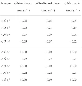
Average a)New theory b)Traditional theory c)No rotation
(mm yr−1) (mm yr−1) (mm yr−1)
<S˙>o −0.05 −0.05 −0.05
<U˙ >o −0.22 −0.24 −0.19
<N˙ >o −0.27 −0.29 −0.24
<G˙ >o −0.05 −0.07 −0.02
<L˙ >e +0.00 +0.00 +0.00
<S˙ >e −0.22 −0.22 −0.21
<U˙ >e +0.00 +0.00 +0.00
<N˙ >e −0.22 −0.22 −0.21
<G˙>e +0.00 +0.00 +0.00
Table 1.Ocean (top) and whole-Earth surface averages (bottom) of the present-day rate of change of GIA fingerprints considered in this study. In this table, the outputs of SELEN4have been rounded to two significant figures. Although in the text we dwelt upon the new rotation theory (columna), results for the the traditional theory are also shown here in (b) while in (c) no rotational effects are taken into account. It is apparent that the spatial averages are only moderately affected by the choice of the rotation theory. The values of<U˙ >e,<G˙ >eand<L˙>eare numerically found to be<10−5mm
Author Contributions:G.S. and D.M. have equally contributed to the development of the theory, to the numerical
543
experiments, and to the writing of the manuscript.
544
Funding:G.S. is funded by a FFABR (Finanziamento delle Attività Base di Ricerca) grant of MIUR (Ministero
545
dell’Istruzione, dell’Università e della Ricerca) and by a research grant of Dipartimento di Scienze Pure e Applicate
546
(DiSPeA) of the University of Urbino “Carlo Bo”.
547
Acknowledgments: Program SELEN4(SELEN version 4.0) is available from Zenodo at the linkhttps:// zenodo.org/
548
record/ 3339209(DOI: 10.5281/ zenodo.3339209) and from the Computational Infrastructure for Geodynamics (CIG)
549
atgithub.com/ geodynamics/selen. The open source Love numbers calculator and Post Glacial Rebound SolverTABOO
550
can be downloaded fromhttps://github.com/danielemelini/TABOO. Some of the figures have been drawn using the
551
Generic Mapping Tools (GMT) of Wessel and Smith [80]. We thank Gaia Galassi and Marco Olivieri for their
552
advice and encouragement. We thank Francesco Mainardi for insightful discussion about the rheological aspects
553
of GIA and for warm hospitality. G.S. has benefited from the serene atmosphere of the Naturalistic Annex of
554
the Museum of Bagnacavallo (RA), Italy, where this paper has been conceived. Raffaello Mascetti has patiently
555
revised the manuscript during various stages of its development, providing constructive comments and invaluable
556
inspiration.
557
Conflicts of Interest:The authors declare no conflict of interest.