Entanglement, Information, Causality
Gennaro Auletta1,a 1University of Cassino, Italy Department Letters and Philosophy
Abstract. The paper is divided in two parts. In the first one a summary of the main issues about quantum non–locality is provided. In the second part, the connections with information and causality are considered. In particular, it is shown that a principle of information causality implies that hyper–correlations among experimental settings are not possible but only correlations among possible outcomes. Since a setting is for measuring a particular observable and the eigenbasis of this observable can be considered a code, this means that information codification is a local procedure.
1 EPR
According to EPR, thecorrectnessof a theory consists in the degree of agreement between its con-clusions and human experience—the objective reality, while itscompletenessis defined as [10]: A theory is complete if every element of objective reality has a counterpart in it. The aim of the EPR article is to show theincompletenessof quantum mechanics in the sense of its inability to give a sat-isfactory explanation of entities which are considered fundamental—in a word, it is a ‘disproof’ and not a positive proof. Indeed, theories can be disproved by experience and (even thought) experiments. The core of the argument is constituted by theSeparability principle, which we can express as fol-lows: Two dynamically independent systems cannot influence each other. The separability principle consists in the assumption that any form of interdependency among physical systems is of dynam-ical and causal type. Therefore, it is important to carefully distinguish the problem of relativistic locality—i.e., the existence of bounds in the transmission of signals and physical effects—from that of separability, which concerns only the impossibility of a correlation between separated systems in the case in which there areno dynamical and causal connections. Part of the EPR argument is that, in the absence of physical interactions, the systems are also separated.
EPR state a sufficient condition for the reality of observables, which can be formulated as follows:
If, without in any way disturbing a system, we can predict with certainty the value of a physical quantity, then, independently of our measurement procedure, there exists an element of the physical reality corresponding to this physical quantity.
The words “without in any way disturbing a system" tells us that the systems are considered as dynam-ically independent. The aim of EPR is to show that, assuming separability and the sufficient condition
ae-mail: [email protected]
DOI: 10.1051/
C
Owned by the authors, published by EDP Sciences, 2014
of reality, quantum mechanics is not complete: in logical terms, for quantum mechanics the following statement holds:
[(Suff. Cond. Reality)∧(Separability)]=⇒ ¬Completeness, (1)
where∧,¬, and the arrow are the logical symbols for conjunction (AND), negation and implication, respectively.
The argument of EPR is structured as follows. From (i) the definition of completeness, (ii) the principles of physical reality and separability, and (iii) the fact that, according to quantum mechan-ics, two non–commuting observables cannot simultaneously have definite values, it follows that the following two statements are incompatible:
• The statementrthat the quantum mechanical description of reality given by the wave function is not complete and
• The statementsthat when the operators describing two physical quantities do not commute, the two quantities cannot have simultaneous reality.
In formal terms,
r s, (2)
where the symbolmeans a XOR. The meaning of the statement (2) is the following: if it is possible to show that two non–commuting observables have in fact simultaneous reality, we can logically conclude that quantum mechanics cannot be a complete description of reality (from the falsity ofswe infer the truth ofr).
Let us consider a one-dimensional systemSmade of two subsystemsS1andS2interacting during
the time interval betweent1andt2, with momenta in the position representations:
ˆ
p(1)x =−ı ∂
∂x1
and pˆ(2)x =−ı ∂
∂x2,
(3)
with momentum eigenfunctions
p1|ϕ=ϕp(x1) and p2|ψ=ψp(x2), (4)
respectively. The vectors|ϕand|ψdescribe the states of the particles 1 and 2, respectively. The eigenfunctions in the position representation are
ϕp(x1)=
1
√
2πe ı
px1 and ψ
p(x2)=
1
√
2πe −ı
(x2−x0)p, (5)
respectively, wherex0is a fixed position (constant) and the eigenfunctionϕp(x1) corresponds to
eigen-value+pwhilstψp(x2) corresponds to the eigenvalue−pof the second particle’s momentum (in other
words, the two particles are moving away from each other with the same direction into opposite senses).
Therefore, the compound system is described by the wave function
Ψ(x1,x2)= +∞
−∞
d pψ−p(x2)ϕp(x1). (6)
Now, I summarize the scheme of the first thought experiment [2, Chap. 16] [4, Chap. 10]:
(b)Therefore, the state (6) reduces to
ψ−p(x2)ϕp(x1). (7)
(c)Then, it is evident that particle 2 must be in stateψ−pand this result can be predicted with absolute
certainty.
(d)However, we were able to formulate such a prediction without disturbing particle 2 (assumption of separability).
(e)Then, as a consequence of (c) and (d) and of the sufficient condition of reality, ˆp(2)x is an element
of reality.
Note that steps (a)–(c) are purely quantum mechanical. Only steps (d)–(e) are connected to the specific EPR argument.
However, if we had chosen to consider another observable of particle 1, say ˆx1, whose
eigenfunc-tions areϕx(x1) (whereasψx(x2) are the eigenfunctions of the observable ˆx2of particle 2), then we
would have written the stateΨof the compound system as
Ψ(x1,x2)=
1
√
2π
+∞
−∞
dxψx(x2)ϕx(x1). (8)
Let us now repeat the previous procedure for the position measurement.
(a’)We locally measure the position on particle 1 and find the eigenvaluex.
(b’)Now it is clear that the state (8) reduces to
ψx(x2)ϕx(x1). (9)
(c’)Then, it is evident that the particle 2 must be in the stateψxand this result can be predicted with
absolute certainty.
(d’)However, we have not disturbed particle 2 (assumption of separability).
(e’)Then, as a consequence of (c’) and (d’) and of the sufficient condition of reality, ˆx(2)is an element
of reality.
Conclusions (e) and (e’) look incompatible on the basis of the fact that position and momentum observables of particle 2 do not commute: going back to Propositionsrands[Eq. (2)], EPR have in this way shown that, assuming thatr(the quantum mechanical description of reality is not complete) is false, sis proved to be false as well since both ˆp(2)x and ˆx(2) have simultaneous reality. Then, the
2 Bohm’s reformulation
The argument as formulate in the original EPR paper is difficult tom test. However, a great step was provided by David Bohm. Consider now two particles with spin1
2 that are in a state in which the total
spin is zero, that is, they are in a singlet state [8]. They can be produced by a single atom radioactive decay. After a timet0the two particles begin to separate and at timet1 they no longer interact. On
the hypothesis that they are not disturbed, the law of angular momentum conservation guarantees that they remain in a singlet state. Considering the projection of the spin along thez–direction, the singlet state may be written in the form
|Ψ0=
1
√
2(| ↑1⊗ | ↓2− | ↓1⊗ | ↑2), (10)
where the subscripts 1 and 2 refer to the particles. This implies that, if a measurement of the spin component along thezdirection of particle 1 leads to a result+1/2, that of particle 2 along the same direction must give the value−1/2, and vice versa. This means that|Ψ0 is an eigenket of thez
component of the spin observables ˆσ1zσˆ2zof the two systems.
Entanglement is a property of the state that is independent of the basis used. In order to see this rotational invariance, let us write it in terms of thez–component eigenvectors as
|Ψ0=
1 √ 2 1 0 1 ⊗ 0 1 2 − 0 1 1 ⊗ 1 0 2 . (11)
Then,|Ψ0turns out to be also an eigenvector of ˆσ1xσˆ2xand ˆσ1yσˆ2y. For example, let us consider the yorientation. First, let us expand thez–eigenkets into they–eigenkets:
|↑ =
√
2 2
|↑y+|↓y
, (12a) |↓ = −ı √ 2 2
|↑y− |↓y
. (12b)
Then, we can write the singlet state (10) in theyexpansion: 1
√
2(|↑1⊗ |↓2− |↓1⊗ |↑2) = 1 √ 2 − ı 2
|↑y+|↓y
1⊗
|↑y− |↓y
2
+ı 2
|↑y− |↓y
1⊗
|↑y+|↓y
2 = √ı 2 |↑y 1⊗ |↓y 2− |↓y 1⊗ |↑y 2 . (13)
Consequently, we have
ˆ
σ1yσˆ2y
|Ψ0 = √ı
2
ˆ
σ1yσˆ2y |↑y
1⊗ |↓y 2− |↓y 1⊗ |↑y 2 , (14)
which, by making use Pauli matrices and of a reformulation of expression (11) in theybasis, implies
ˆ
σ1yσˆ2y
|Ψ0 = ı
2√2
0 −ı
ı 0
1
0 −ı
ı 0 2 × 1 ı 1 ⊗ 1 −ı 2 − 1 −ı 1 ⊗ 1 ı 2 = ı
2√2
1 ı 1 ⊗ −1 ı 2 − −1 ı 1 ⊗ 1 ı 2 = √ı 2 |↑y 1⊗
− |↓y
2−
− |↓y
Now, let us back–substitute this expression into thezexpansion:
ı
√
2
|↑y
1
− |↓y 2−
− |↓y
1
|↑y 2
= −√ı
2 1 2
(|↑+ı|↓)1(− |↑+ı|↓)2
−(− |↑+ı|↓)1(|↑+ı|↓)2
= √ı
2(ı|↑1|↓2−ı|↓1|↑2)
= −√1
2(|↑1|↓2− |↓1|↑2)
= −|Ψ0, (16)
where I have dropped the symbol⊗of the sake of simplicity.
3 Bell Theorem
Bell assumed the existence of a hidden parameterλsuch that, givenλ, the functionAadescribing the
results obtained by measuring with a deviceAthe spin of the first particle along a chosen direction a(i.e., the observable ˆσ1·a), depends only onλand ona[6]. Similarly, the function Bbdescribing
the results when measuring with a deviceBthe spin of the second particle along a chosen direction b(i.e., ˆσ2·b), depends only onbandλ. The separability principle denies that there can be a form of
interdependence between two systems if they do not dynamically interact (factorization rule):
AaBb=Aa(λ)Bb(λ), (17)
where thereforeAa andBbrepresent two deterministic functions of the hidden parameter. Eq. (17)
expresses the fact that the probability distributions for the two particles are mutually independent. I assume that the result of each measurement can be either+1 (representing spin up) or -1 (representing spin down), that is,
Aa(λ)=±1, Bb(λ)=±1. (18)
Following Eq. (17), if℘(λ) denotes the probability distribution of the hidden parameterλ, then the expectation value of the product of the two components ˆσ1·aand ˆσ2·bis
( ˆσ1·a) ( ˆσ2·b)=
Λ℘(λ)Aa(λ)Bb(λ)dλ, (19)
whereΛrepresents the set of all possible values ofλ.
In the present context,Aa(λ) and Bb(λ) are functions defining the possible measurement results
or the eigenvalues of the measured observables. Since we do not know the values of the hidden parametersλ, we must integrate over all the possible valuesλ∈Λ. Because℘(λ) is supposed to be a normalized probability distribution, we have
Λ℘(λ)dλ=1, (20)
and, given the values (18), we also have
where I have rewritten the expression( ˆσ1·a) ( ˆσ2·b) in the simplified form a,b. Our aim is to
compare the prediction of a deterministic HV theory as expressed by Eq. (19) with the quantum mechanical expectation value, which for the singlet state|Ψ0[Eq. (10)] is given by
a,bΨ0 =Ψ0|( ˆσ1·a) ( ˆσ2·b)|Ψ0=−a·b. (22)
This result can be derived when considering the previous products between observables and vectors as sum of Cartesian components
ˆ
σ1·a = ax
0 1 1 0
1
+ay
0 −ı
ı 0
1
+az
1 0
0 −1
1
, (23a)
ˆ
σ2·b = bx
0 1 1 0
2
+by
0 −ı
ı 0
2
+bz
1 0
0 −1
2
, (23b)
The expectation value on the singlet state (11) of these two products gives 9 terms, of which the first three have the form
Ψ0|axbxσˆ1xσˆ2x|Ψ0 = Ψ0| axbx
√ 2 0 1 1 0 1 0 1 1 0 2 × 1 0 1 ⊗ 0 1 2 − 0 1 1 ⊗ 1 0 2
= Ψ0|−axbx|Ψ0=−axbx. (24)
Indeed, similar calculations show that we also have
Ψ0aybyσˆ1yσˆ2yΨ0
=−ayby and Ψ0|azbzσˆ1zσˆ2z|Ψ0=−azbz. (25)
The remaining six cross terms are instead all zero, so that we may finally conclude that
Ψ0|( ˆσ1·a) ( ˆσ2·b)|Ψ0 = −(axbx+ayby+azbz)=−a·b. (26)
When the two orientationsaandbare parallel, quantum mechanical calculations [see Eq. (15)] show that
a,aΨ0 =−1, (27)
as it should be since there is a perfectanticorrelation(spin–up versus spin–down) between the results of the two measurements.
Since the value given by Eq. (27) for perfect anticorrelation is an experimental fact, also a HV theory must satisfy this requirement. On the other hand,a,a=−1 holds if and only if we also have
Aa(λ)=−Ba(λ), (28)
for any directiona. In this case, Eq. (19) reaches the minimum value [see also Eq. (21)]. Under this assumption, we can drop any reference to theBdevice and rewrite Eq. (19) as
a,b=−
dλ℘(λ)Aa(λ)Ab(λ). (29)
Now we consider two alternative orientations, saybandc, of the spin measurement of particle 2:
a,b − a,c = −
dλ℘(λ)[Aa(λ)Ab(λ)−Aa(λ)Ac(λ)]
=
because of the property (18) and since, for any orientationn, we have [An(λ)]2=1, which implies
Aa(λ)Ab(λ)Ab(λ)Ac(λ)=Aa(λ)Ac(λ). (31)
Then, from Eq. (30) we may prove the inequality
| a,b − a,c | ≤
dλ℘(λ)[1−Ab(λ)Ac(λ)]. (32)
This result is obtained when one considers that for any integrable function f(x), we have
dx f(x) ≤
dx|f(x)|, (33)
and, given again the property (18), we also have
|Ab(λ)Ac(λ)−1|=1−Ab(λ)Ac(λ). (34)
Therefore, given the property (20) we finally obtain
| a,b − a,c | ≤1+b,c, (35)
where
b,c=−
dλ℘(λ)Ab(λ)Ac(λ). (36)
A reformulation of the Bell inequality (35) is the so-called CHSH inequality, a widely used form,
a,b+a,b+a,b−a,b≤2, (37)
wherea is a setting alternative to a as well as b to b. We may associate to this inequality the following Bell operator:
ˆ
B=σˆ1·a
ˆ
σ2·b+σˆ2·b
+
ˆ
σ1·a
ˆ
σ2·b−σˆ2·b
=( ˆσ1·a) ( ˆσ2·b)+( ˆσ1·a)σˆ2·b
+σˆ1·a( ˆσ2·b)+σˆ1·a σˆ2·b, (38)
which will play a crucial role later on. I recall indeed that e.g.a,bis a shorthand for( ˆσ1·a) ( ˆσ2·b),
which allows us to write
Bˆ≤2. (39)
4 Experiments and Loopholes
Tests of the Bell theorem already started in the mid of 1970s. However, several loopholes were dis-covered that affected these early experiments and could be dealt with step by step. Thefirst loophole
we consider is the locality loophole. In all experiments, one should consider the possibility that the result of a measurement obtained by using a certain polarizer direction depend on the orientation of the other polarizer. This problem was overcome by Aspect’s team [1] as outlined in Fig. 1.
coincidence coincidence S
A(a) B(b)
γA γB
DA DB
C A C B
A 1(a ) B (1 b )
S γ
A γB
1 l 1
A2 2 (a ) B2 (b 2)
DA 2 DB 2
DA 1 DB 1
(a) (b)
Figure 1.One should consider the possibility that the results obtained using a certain polarization direction could depend on the other polarizer. (a) Friedman–Clauser experiment: The correlated photonsγA, γBcoming from the source S impinge upon the linear polarizersA,Boriented in directionsa,b, respectively. (b) Experiment proposed by Aspect: The optical commutator CAdirects the photonγAeither towards polarizerA1 with orientationa1 or to polarizerA2 with orientationa2. Similarly for CBforB1andB2. The two commutators work independently (the time intervals between two commutations are taken to be stochastic). The four joint detection rates are monitored and the orientationsa1,a2,b1,b2are not changed for the whole experiment.lis the separation between the switches.
KDP UV
UVF
C NDF 90° Rot.
1 C
2
Pol.θ1
Pol.θ 2
IF
IF D2 D1
i
s
Ampl.
Counter
Counter TDC PDP
11/23+ BS
Ampl. M1
M2
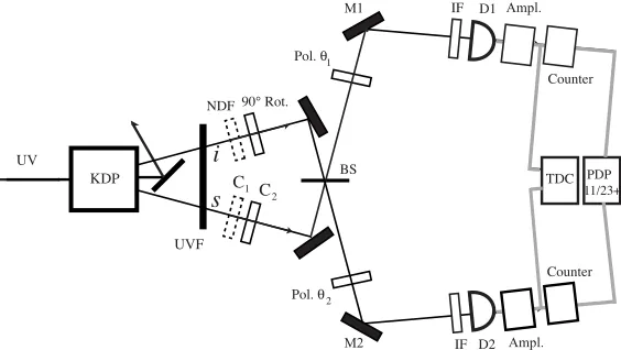
Figure 2.Because of the cosine–squared angular correlation of the directions of the photons emitted in an atomic cascade, an inherent polarization decorrelation is present. Outline of the Alley–Shih and Ou–Mandel’s experiment. Light from the 351.1– nm line of an argon–ion laser falls on a non–linear crystal of potassium dihydrogen phosphate (KDP), where down-converted photons of wavelength of about 702 nm are produced. Down–conversion can be tuned in order that linearly polarized signal and idler photons emerge at angles of about±2◦relative to the ultraviolet (UV) pump beam with the electric vector in the plane of the diagram. Theidler(i) photons pass through a 90◦polarization rotator, while thesignal(s) photons traverse a compensating glass plate C1producing an equal time delay. The two photons are then directed from opposite sides towards a beam splitter (BS). The input to the BS consists of anx–polarized s–photon and of a rotatedy–polarized i–photon. The light beams emerging from BS, consisting of a mixing of i-photons and s-photons, pass through linear polarizers set at adjustable anglesθ1andθ2, through similar interference filters (IF) and finally fall on two photodetectors D1and D2. The photoelectric pulses from D1and D2are amplified and shaped and fed to the start and stop inputs of a time-to-digital converter (TDC) under computer control which functions as a coincidence counter.
violation of one of the Bell inequalities is reduced for non–collinear photons. The problem can be overcome by using SPDC sources instead of atomic cascade ones [14]. Pairs of photons resulting from SPDC can have an angular correlation of better than 1 mrad, although in general they need not be collinear. The set up is shown in Fig. 2.
PBS
NL Type-II Phase Match.
|v>2
|v>1
|h>1
|h>2
|v>3 |h>3
|v>4 |h>4
Translatable mirror
PBS
Optional HWP
(a)
UV-blocking filter
HWP, α
PBS UV pump
(b)
High-efficiency detectors
Collection lens Collection lens
spatial filters
φ 1
2
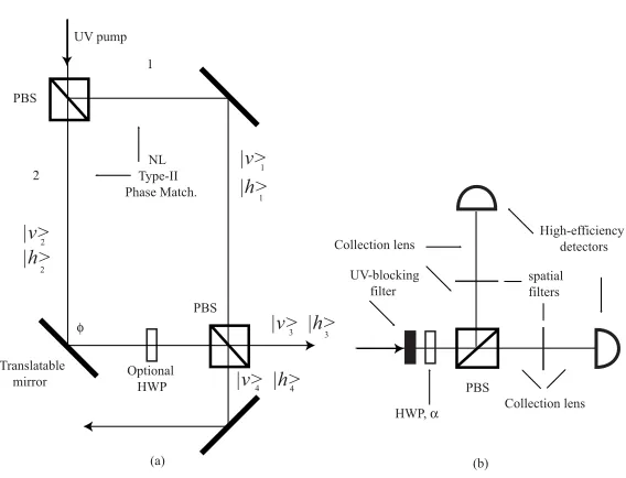
Figure 3. The question is how high the detection efficiency must be for the experimental confirmation of the quantum predictions. In Aspect’s experiment the required is 83%. With SPDC experiments, we are obliged to discard part of the counts (when both photons are in the same channel). Proposed experiment for solving the detection loophole. A possible solution is to directly produce a pair of photons in a singlet–kind state avoiding in this way any post–selection.
(a) An ultraviolet pump photon may be spontaneously down-converted in either of two nonlinear crystals, producing a pair of collinear orthogonally polarized photons at half the frequency (type–II phase matching). The outputs are directed toward a second PBS. When the outputs of both crystals are combined with an appropriately relative phaseφ, a true singlet- or triplet-like state may be produced. By using a half-wave plate (HWP) to effectively exchange the polarizations of photons originating in crystal 2, one overcomes several problems arising from nonideal phase matching. An additional mirror is used to direct the photons into opposite direction towards separated analyzers.
(b) A typical analyzer, including an HWP to rotate byθthe polarization component selected by the analyzing BS, and precision spatial filters to select only conjugate pairs of photons. In an advanced version of the experiment, the HWP could be replaced by an ultrafast polarization rotator (such as Pockels or Kerr cells) to close also the locality loophole.
quantum theoretical predictions. The problem with SPDC–type experiments is that, even with high detection efficiency, one must discard part of the counts, since we are obliged to discard all events where both photons are in the same channel, and one could rise the question whether this selection might represent a bias. Even though this is a remote possibility, in order to exclude any ambiguity a more refined solution is required [12]. A possibility is to directly produce a pair of photons in singlet– type state, thus avoiding any post–selection. One of the first proposals for doing this is shown and summarized in Fig. 3. By means of this apparatus it is possible to produce output photons in the state
|Ψ |v3|h4+eıφ(|h3|v4) . (40)
5 Non–Locality and Information
I have a general remark. Given any quantum system described by the density matrix ˆρ, its von Neu-mann entropy is [11]
S( ˆρ)=−Tr( ˆρln ˆρ). (41)
ˆ
ρfor a systemSsuch that
ˆ
ρ|bk=rk|bk , (42)
where therk’s are the eigenvalues of ˆρ, we may rewrite Eq. (41) as
S( ˆρ)=−
j
rjlnrj, (43)
The eigenvectors|bkare the possible outcomes of a measurement when we choose to measure the
observable of which they are eigenvectors. Let us define the entanglement between systems [5] 1 and 2 as
E(1,2) = S(1,2)−S(1)−S(2), (44)
whereS(1,2) is the joint (total) entropy of systems 1 and 2, and
S(1)=S( ˆ1) and S(2)=S( ˆ2) (45)
are the entropies calculated on the reduced density matrices of the subsystems 1 and 2, respectively, relative to ˆρ12. This reflects the fact that entanglement is a quantum form of mutual information: Two
entangled systems are correlated because they share an amount of information that is not foreseen classically: indeed the possible outcomes are interdependent.
Are there specific quantum mechanical bounds on information acquisition? Is the bound found with inequality (35) a necessity or are there more rigorous bounds? And if they are, what is their meaning? Let us take advantage of the CHSH inequality (37). Since each of the terms in Eq. (37) lies between−1 and+1 [Eq. (21)], the natural upper bound for the entire expression is+4. This is precisely the case if we demand that the probabilities satisfy only the causal communication constraint [16], i.e., that they do not violate relativistic locality (what is called non–signaling requirement). In this case, we have
a,b+a,b+a,b−a,b≤4 or Bˆ≤4. (46)
Indeed, the non–signaling requirement is that the operations one can perform locally here are not influenced by the operations one performs elsewhere, which implies in particular that the probability to obtain a certain outcome (say 1) when choosing the directionais independent from the outcomes (either+1 or -1) when elsewhere one choses a directionborb, that is,
℘a,b(1,1)+℘a,b(1,−1)=℘a,b(1,1)+℘a,b(1,−1). (47)
Similar considerations hold for any direction. If we consider only this requirement, we are allowed to build the set of probabilities
℘a,b(1,1)=℘a,b(−1,−1)=
1
2 , ℘a,b(1,1)=℘a,b(−1,−1)= 1 2
℘a,b(1,1)=℘a,b(−1,−1)=
1
2 , ℘a,b(1,−1)=℘a,b(−1,1)= 1
2, (48)
while all other probabilities are zero and where I remark that only the℘a,bprobabilities show anti–
correlation.
All the four different expectation values in inequality (46) can be formulated as the following one:
where the negative sign of the latter two probabilities is due to the fact that both represent anticor-relations. However, this expectation value in the paramount case in which all probabilities are equal mirrors the separability condition (17), i.e., the absence of correlations (a,b=0) between the two systems. Due to the above assumptions, however, the latter two probabilities are zero so that the whole expression is reduced to
a,b=℘a,b(1,1)+℘a,b(−1,−1), (50)
and similarly for the other three correlations. In this way, taking into account the probabilities (48), the upper bound 4 of inequality (46) is easily obtained.
Let ˆOa,Oˆa,Oˆb,Oˆbbe arbitrary Hermitian operators on a Hilbert spaceHsatisfying the condition
[ ˆOa,Oˆb]=0 and so on for the other couples (a,b),(a,b),(a,b) [17]. Moreover, each operator has eigenvalues 1 and−1. We define a generalization of the Bell operator (38), since we are no longer considering the spin observable only,
ˆ
B=OˆaOˆb+OˆaOˆb+OˆaOˆb−OˆaOˆb. (51)
From the previous assumptions, it follows that the square of each operator is equal to the identity, which implies
2√2−Bˆ = √1 2
( ˆOa)2+( ˆOa)2+( ˆOb)2+( ˆOb)2−Bˆ
= √1
2
⎡ ⎢⎢⎢⎢⎢ ⎣
ˆ
Oa−Oˆb+Oˆb √
2
2
+
ˆ
Oa−Oˆb−Oˆb √
2
2⎤ ⎥⎥⎥⎥⎥
⎦=Aˆ. (52)
Now, we wish to prove that ˆB can be expanded as above and that:
Bˆ≤2√2. (53)
Let us expand the operator ˆA as
1
√
2
⎡ ⎢⎢⎢⎢⎢ ⎢⎢⎢⎣( ˆOa)2+
ˆ
Ob+Oˆb2
2 −2
ˆ
OaOˆb+Oˆb √
2 +( ˆO
a)2+
ˆ
Ob−Oˆb2
2 −2
ˆ
OaOˆb−Oˆb √
2
⎤ ⎥⎥⎥⎥⎥ ⎥⎥⎥⎦
= √1
2 · 1
2√2
2√2( ˆOa)2+√2( ˆOb)2+√2( ˆOb)2+2√2 ˆObOˆb−4 ˆOaOˆb−4 ˆOaOˆb
+2√2( ˆOa)2+√2( ˆOb)2+ √2( ˆOb)2−2√2 ˆObOˆb−4 ˆOaOˆb+4 ˆOaOˆb
= 1 4
2√2( ˆOa)2+√2( ˆOb)2+ √2( ˆOb)2+2√2( ˆOa)2+√2( ˆOb)2+ √2( ˆOb)2
+2√2 ˆObOˆb−2√2 ˆObOˆb−4 ˆOaOˆb−4 ˆOaOˆb−4 ˆOaOˆb+4 ˆOaOˆb
= 1 4
2√2( ˆOa)2+( ˆOb)2+( ˆOa)2+( ˆOb)2−4OˆaOˆb+OˆaOˆb+OˆaOˆb−OˆaOˆb
= 1 4
8√2 ˆI−4 ˆB. (54)
This proves the expansion of ˆB. Now, consider that the sum or the difference between Hermitian operators is itself a Hermitian operator, which shows that the following two operatorial expressions are Hermitian:
ˆ
Ob+Oˆb √
2 and
ˆ
Ob−Oˆb √
The last step implies that also
ˆ
Oa−Oˆb+Oˆb √
2 and
ˆ
Oa−Oˆb−Oˆb √
2 (56)
are. Therefore, the operator
ˆ A= √1
2
⎡ ⎢⎢⎢⎢⎢ ⎣
ˆ
Oa−Oˆ
b+Oˆb √
2
2
+
ˆ
Oa−Oˆ
b−Oˆb √
2
2⎤ ⎥⎥⎥⎥⎥
⎦, (57)
which consists of the sum of squares of Hermitian operators, has clearly an expectation value
ˆ
A≥0. (58)
Since by taking the mean value on both sides of Eq. (53) we have
ˆ
A=2√2−Bˆ, (59)
this leads to the conclusion:
ˆ
B ≤ 2√2. (60)
A similar argument leads to
ˆ
B ≥ −2√2, (61)
which finally implies
Bˆ≤2√2. (62)
The importance of Tsirelson result lies in the fact that it proves that quantum mechanicsdoes not
fill the entire gap between the bounds set by Eqs. (37) and (46). The former inequality sets bounds (i.e., 2) for classical separable theories whilst quantum mechanics satisfy the bound 2√2, which is still stricter than the bound (i.e., 4) imposed by inequality (46). In other words, quantum mechanics certainly allows for correlations that are not allowed by classical HV theories. However, there is a wide spectrum of "hyper–correlations" that do not contradict causal communication constraints (they satisfy the bound imposed by inequality (46)) but are nevertheless not allowed by quantum mechanics (since they do not satisfy inequality (62)). Therefore, we need still to clarify the relations between these different bounds.
To examine this point, let us reformulate the CHSH inequality (37) as an equality with the maximal bound attainable, i.e., B=2, which could be rewritten as [13]
1
2B−1=0, (63)
where B expresses again the Bell operator written in terms of a numerical parameter B. However we are interested in more general cases than those allowed by the classical separability requirement. In those case, instead of putting a 0 on the right-hand side we write another numerical parameter, D, as follows:
D=1
2B−1. (64)
Moreover, we like to write the parameter B as a combination of correlations Cjk (where j,k =
possible outputs when Alice and Bob measure in informational term 1,0. In other words, instead of speaking of polarization directionsa,a,b, andb, or of observables ˆOa,Oˆa,Oˆb,Oˆb, we would like to
introduce generic inputsa,b =0 anda,b=1. Moreover, instead to have possible results−1,1, we like to introduce information outputs 0,1. With these assumptions, we rewrite the correlationa,bfor the non–signaling case as expressed in the formula (50) as the sum of two conditional probabilities:
C00=℘(11|00)+℘(00|00), (65a)
where what follows the vertical lines are the inputs and what precedes the vertical line the outputs. Similarly, we have
C10=℘(11|10)+℘(00|10), C01=℘(11|01)+℘(00|01), C11=℘(10|11)+℘(01|11),
where the first equality is a reformulation of the correlationa,b, the second of the correlationa,b, and the latter of the correlationa,b, and again I remark that only the latter one is an anticorrelation.
Then we can write:
D = 1
2B−1 = 1
2(C00+C01+C10−C11)−1. (66)
Let us now introduce a simplification. In the case in which
C00=C01=C10=−C11≥0, (67)
we can write
C=C00=C01=C10=−C11, (68)
which implies B=4C (or C=B/4) that allows us to make the parameter D dependent on C and to rewrite the expression (66) as
D(C)=1
2 ·4C−1 = 2C−1. (69)
It is easy to see that
• When C=1 we also have D=1, which implies that Bns=4, which is precisely the non–signaling
case (when only the causal requirement in the transmission of signals is observed).
• Instead, we have the classical separability Bc=2 when C=1/2 and D=0. • In the quantum case, we have Bq=2
√
2 when C=1/√2 and D= √2−1.
To have a concrete model, let us briefly consider how teleportation works [7]. The eigenbasis of the Bell operator is given by
Ψ−
12 =
1
√
2(|↑1|↓2− |↓1|↑2), (70)
Ψ+
12 =
1
√
2(|↑1|↓2+|↓1|↑2), (71)
Φ−
12 =
1
√
2(|↑1|↑2− |↓1|↓2), (72)
Φ+
12 =
1
√
I
1
2
3
4 +
Φ
_Φ
_
Ψ
+
Ψ
particle 1 input
measurement results on particles 1-2
operations on particle 3
U
U
U
U
I
particle 3 output
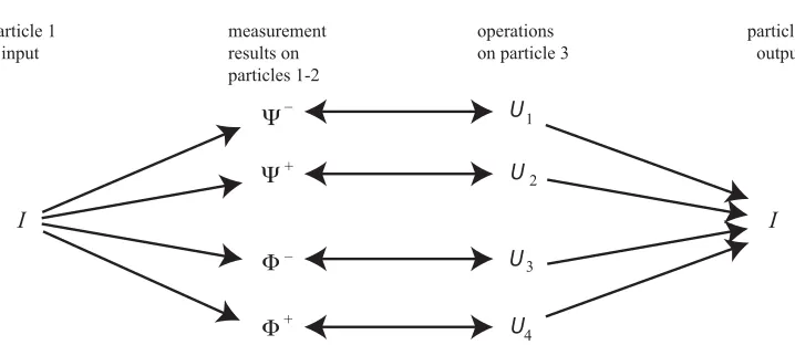
Figure 4. Scheme of teleportation: the fact that each measurement result is mapped in a certain way to the input informationI allows through the ebit that Alice classical instructs Bob about the kind of operation to be performed. It is a code.
The state of the three particles can be described as
|Ψ123 =
1 2Ψ
−
12
−
c|↑3−c|↓3 +Ψ+
12
−
c|↑3+c|↓3
+Φ−
12
c|↓3+c|↑3 +Φ+
12
c|↓3−c|↑3
.
(74)
It suffices an unitary operation (a mechanical instruction) to recover the information of Particle 1 on 3 once the Bell operator has been measured:
ˆ
U1=
−1 0
0 −1
; Uˆ2=
−1 0
0 1
; Uˆ3=
0 1 1 0
; Uˆ4=
0 1
−1 0
(75)
We can assume an information causality principle which (in a teleportation protocol) relates to the amount of information that Bob can gain about a data set belonging to Alice, the contents of which are completely unknown to him [15]. Using all his local resources (which may be correlated with her resources) and allowing classical communication from Alice to Bob, the amount of information that the latter can recover is bounded by the information volume (n) of the communication. Namely, if Alice classically communicatesnbits to Bob, the total information obtainable by Bob cannot be greater thann. Consider the easiest case in which a two-bit information has been classically transmit-ted. Then, Bob can at most recover this information (the instruction to perform a particular unitary operation out of four on his particle) and not the whole set of potential information from which Alice has selected the message she has sent. Then, in this simple case, the acquired information must be bound as
I≤2, (76)
Let ˆO1 and ˆO2 be two observables on subsystemsS1 andS2 of a system S, respectively, and ℘(oa,a;ob,b) be the probability that the results of a measurement of ˆO1 onS1 and ˆO2 onS2yield oa andob when certain settings of the measurement apparata area andb, respectively. Since this
assumption is of absolute generality, we not need to consider the specific spin model previously intro-duced.
According to Eberhard, the probability distribution of ˆO1(or ˆO2), independently of the
measure-ment operations on ˆO2 (or ˆO1), obtained by integrating or summing the probabilities℘(oa,a;ob,b)
over the possible outcomesob(oroa), needs to be independent of the other settingb(ora), that is, the
two probabilities must depend on local settings only [9]:
ob℘(oa,a;ob,b)=℘(oa,a) ;
oa℘(oa,a;ob,b)=℘(ob,b). (77)
According to Eberhard, if this requirement were violated, we would have acausal non–local inter-dependencebetween the two subsystems. Actually, a violation of the above requirement does not necessarily imply a non–local causal interconnection because there could still be a form of interde-pendence but satisfying the non–signaling requirement.
In order to prove the theorem, let
ˆ
Poa,a=|oa,a oa,a| and Pˆob,b=|ob,b ob,b| (78)
be the projectors on the state|oa,aof subsystemS1when the setting isaand the outcome|oa, and
on the state|ob,bof subsystemS2when the setting isband the outcome|ob, respectively, and ˆρa
density matrix which represents the compound state ofS=S1+S2. The probability℘(oa,a) that, by
measuring the observable ˆO1onS1, we obtain the outcome|oa(or the eigenvalueoa), is
℘(oa,a)=Tr
ˆ
Poa,aρˆ
. (79)
After a measurement of ˆO1when the setting isawith resultoawe obtain the transformation
ˆ
ρ→ρˆ=Pˆoa,aρˆPˆoa,a
℘(oa,a) .
(80)
If we perform a second measurement on the second subsystem, the conditional probability of obtain-ing|ob(orob) by measuring ˆO2when the setting isb, is given by
℘(o
b,b|oa,a)=Tr
ˆ
Pob,bρˆ
= Tr
ˆ
Pob,bPˆoa,aρˆPˆoa,a
℘(oa,a) .
(81)
For any eventsAandB, the classical probability calculus tells us that the probability of their joint occurrence can be expressed as
℘(A,B)=℘(A)℘(B|A). (82)
Therefore, the joint probability of obtaining the two resultsoa andob given the settingsaandb, is
given by combining Eqs. (79) and (81):
℘(oa,a;ob,b) = ℘(oa,a)℘(ob,b|oa,a)
= ℘(oa,a)
TrPˆob,bPˆoa,aρˆPˆoa,a
℘(oa,a)
= TrPˆob,bPˆoa,aρˆPˆoa,a
Given these assumptions, we can obtain the following result that is in accordance with Eqs. (77):
oa
℘(oa,a;ob,b)=Tr
oa
ˆ
Pob,bPˆoa,aρˆPˆoa,a
=TrPˆob,bρˆ
=℘(ob,b). (84)
To derive this result, first note that
oa
TrPˆob,bPˆoa,aρˆPˆoa,a
=Tr
oa
ˆ
Pob,bPˆoa,aρˆPˆoa,a
. (85)
Moreover, I have made use of the cyclic properties of the trace, i.e., given any three arbitrary observables, we have
TrOˆ1Oˆ2Oˆ3
=TrOˆ3Oˆ1Oˆ2
=TrOˆ2Oˆ3Oˆ1
. (86)
This property implies that
Tr
oa
ˆ
Pob,bPˆoa,aρˆPˆoa,a
=Tr
oa
ˆ
Poa,aPˆob,bPˆoa,aρˆ
. (87)
Moreover, ˆPoa,a and ˆPob,b commute because they pertain to different subsystems, and therefore we
have
Tr
oa
ˆ
Poa,aPˆob,bPˆoa,aρˆ
=Tr
oa
ˆ
Pob,bPˆoa,aPˆoa,aρˆ
. (88)
However, any orthogonal set of projectors {Pˆoa,a} satisfies the two properties ˆPo2a,a = Pˆoa,a and
oaPˆoa,a =Iˆ, from which we finally obtain
Tr
oa
ˆ
Pob,bPˆoa,aPˆoa,aρˆ
=TrPˆob,bρˆ
. (89)
We may proceed in a similar way starting from the conditional probability℘(oa,a|ob,b) in order to
derive the second equality (77).
What would happen in a world in which the quantum bound is violated but the locality (non– signaling) requirement is satisfied [3]? Let us now reformulate the quantum–mechanical Eqs. (77) in analogy with Eq. (47) as
℘a,b(1,1)+℘a,b(1,−1)=pa(1) and ℘a,b(1,1)+℘a,b(−1,1)=℘b(1), (90)
and similarly for the other outcomes. This clearly shows that quantum mechanics requires a full independence of the settings (here expressed by the orientationa), which need to be local operations performed in complete separation from other operations that could be performed elsewhere. Quantum correlations are indeed interdependencies of possible outcomes and not of settings. In other words, a violation of the quantum mechanical bound (and of the information causality principle) would imply that there are correlations between settings. If we consider the abstract forms (65) in which I have written the correlations entering in the CHSH inequality, we see that they are expressed in terms of pure conditional probabilities of the form℘(11|00) Following the customary approach in quantum mechanics (and our physical experience) we have naturally interpreted probabilities of this form as expressing e.g. the probability that both Alice and Bob get the output 1 given that they have both chosen the setting 0. In fact, if Bob knows which was the setting of Alice (whether 0 or 1) he is able to infer which was her outcome. On this procedure is indeed based quantum cryptography.
• If Bob choses the setting 0, obtains the outcome 0 and knows that A has also obtained the outcome 0, he knows that she has chosen the setting 0;
• If Bob choses the setting 1, obtains the outcome 0 and knows that A has also obtained the outcome 0, he knows that she has chosen the setting 1;
• If Bob choses the setting 0, obtains the outcome 0 and knows that A has obtained the outcome 1, he knows that she has chosen the setting 0;
• If Bob choses the setting 1, obtains the outcome 0 and knows that A has obtained the outcome 1, he knows that she has chosen the setting 1;
• If Bob choses the setting 0, obtains the outcome 1 and knows that A has obtained the outcome 0, he knows that she has chosen the setting 0;
• If Bob choses the setting 1, obtains the outcome 1 and knows that A has obtained the outcome 0, he knows that she has chosen the setting 1;
• If Bob choses the setting 0, obtains the outcome 1 and knows that A has also obtained the outcome 1, he knows that she has chosen the setting 1;
• If Bob choses the setting 1, obtains the outcome 1 and knows that A has also obtained the outcome 1, he knows that she has chosen the setting 0.
6 Conclusion
In a world in which settings (and not only outcomes) are shared and so there would be kinds of non– local settings, this would imply that also information codification is shared. Indeed, it can be shown that information codification deals with the choice of a basis which in a measurement context is the choice of a setting. In other words, in a world showing hyper–correlations based on the sharing of settings, information codification would be no longer a local procedure.
The fact that this is forbidden justifies quantum information as a general theory of information since
• It satisfies and saturates the bounds that are imposed by the principle of information causality, and in so doing
• It also sets specific constraints on both the possible interdependencies and the possible interactions (also causal interconnections) in our universe.
The most general conclusion is that information can be defined as correlation among possible out-comes or events, as we have seen above for the mutual–information expression of entanglement.
References
[1] Aspect, A. , Dalibard, J., and Roger, G., Physical Review Letters49, 1804–1807 (1982).
[2] Auletta, G., Fortunato, M., and Parisi, G., Quantum Mechanics(Cambridge University Press, Cambridge, 2009).
[3] Auletta, G., Journal of Modern Physics2, 958–61 (2011).
[4] Auletta, G. and Wang, S.–Y.,Quantum Mechanics for Thinkers(PanStanford Pub., Peking, 2013). [5] Barnett, S. M. and Phoenix, S. J. D., Physical ReviewA40, 2404–2409 (1989).
[6] Bell, J. S., Physics1, 195–200 (1964).
[8] Bohm, D.,Quantum Theory(Prentice-Hall, New York, 1951). [9] Nuovo Cimento46B, 392–419 (1978).
[10] Einstein, A., Podolsky, B., and Rosen N., Physical Review47, 777-780 (1935). [11] Fano, U., Review of Modern Physics29, 74–93 (1957).
[12] Kwiat, P. G., Eberhard, P. H., Steinberg, A. M., and Chiao, R. Y., Physical ReviewA49, 3209–20 (1994).
[13] Masanes, L., Acin, A., and Gisin, N., Physical ReviewA73, 012112-1–9 (2006). [14] Ou, Z. Y. and Mandel, L., Physical Review Letters61, 50–53 (1988).
[15] Pawłowski, M., Paterek, T., Kaszlikowski, D., Scarani, V., Winter, A., Zukowski, M. Z., Nature 461, 1101–1104 (2009).