Article
1
Visual head counts: a promising method for efficient
2
monitoring of diamondback terrapins
3
Patricia Levasseur 1*, Sean Sterrett 2 and Chris Sutherland 1,*
4
1 Department of Environmental Conservation, University of Massachusetts - Amherst ;
5
[email protected] (P. L); [email protected] (C. S)
6
2 Department of Biology, Monmouth University; [email protected]
7
* Correspondence: [email protected] (C. S); [email protected] (P. L)
8
9
Abstract: Generating a range-wide population status of the diamondback terrapin (Malaclemys
10
terrapin spp.) is challenging due to a combination of species ecology and behavior, and limitations
11
associated with traditional sampling methods. Visual counting of emergent heads offers an efficient,
12
non-invasive and promising method for generating abundance estimates of terrapin populations
13
across broader spatial scales and can be used to explain spatial variation in population size. We
14
conducted repeated visual head count surveys at 38 predetermined sites along the shoreline of
15
Wellfleet Bay in Wellfleet, Massachusetts. We analyzed the count data using a hierarchical modeling
16
framework designed specifically to analyze repeated count data: the so-called N-mixture model.
17
This approach allows for simultaneous modeling of imperfect detection to generate estimates of true
18
terrapin abundance. We found detection probability was lowest when skies were overcast and when
19
wind speed was highest. Site specific abundance varied but we found that abundance estimates
20
were, on average, higher in unexposed sites compared to exposed sites. We demonstrate the utility
21
of pairing visual head counts and N-mixture models as an efficient method for estimating terrapin
22
abundance and show how the approach can be used to identifying environmental factors that
23
influence detectability and distribution.
24
Keywords: abundance, detection, diamondback terrapin, Malaclemys terrapin, monitoring,
N-25
mixture, salt marsh, visual head count
26
27
1. Introduction
28
The diamondback terrapin (DBT; Malaclemys terrapin spp.) is the only estuarine obligate turtle
29
species in North America [1], and as a result, has a long but fragmented coastal range that extends
30
from Cape Cod, Massachusetts, to the Texas Gulf Coast [2]. DBT are currently listed as protected or
31
regulated in every range state [3]. Despite their conservation status, population assessments have
32
been limited to local scales, and as a result, range wide inference about the status of this imperiled
33
species is generally lacking [3,4].
34
As salt marsh specialists, DBT have specific life history and behavioral traits that determine
35
which monitoring techniques are suitable and how that data can be used. For example, DBT have
36
highly seasonal phenology in their northern range [5], form mating aggregations [6], and have highly
37
specialized terrestrial nesting habitat requirements. The species is highly mobile [1] responding
38
locally to disturbance when at the surface but also making larger movements with the tides, and they
39
use regular surface breathing bouts as a behavioral adaptation to brackish conditions [3]. A variety
40
of methods are used to monitor DBT, including modified crab traps [7–9], hoop traps [10,11], trammel
41
nets [4,10–12], fyke nets [13,14], seins [12,15,16] and dip nets [8,11]. While each method takes some
42
aspects of DBT ecology into consideration, their success, in terms of consistent, reliable, and scalable
43
population estimates has been variable. For example, in Wellfleet Bay (MA), almost four decades of
44
monitoring using capture mark recapture (CMR) has resulted in over 3,000 marked individuals [17],
45
but failed to produce reliable estimates of population sizes due to low detection rates (see also:
46
[9,11,16]), mature female biased captures (see also: [7,18]), and variable and opportunistic search
47
effort. These challenges often result in extensive sampling effort being concentrated in very small
48
study areas that are not representative of the landscape, and therefore are not appropriate for
49
landscape of range scale inferences [16,18,19].
50
A promising, but vastly under-utilized, monitoring method for DBT is visual counting of
51
emergent heads (hereafter, visual head counts), which offers an efficient, non-invasive method for
52
generating abundance estimates of local populations. Because DBT are the only turtle species to
53
inhabit coastal estuarine habitats, must surface to breathe air, and perform seasonal staging behavior
54
where both sexes congregate to initiate courtship and mating, their biology and behavior lend
55
themselves naturally to count-based methods that do not require individual recognition. Visual
56
(point) count surveying is a established monitoring method in avian ecology [20], with
well-57
developed field protocols that can easily be modified for DBT; and well-developed statistical models,
58
the so-called N-mixture model, for analyzing exactly the type of data that arise from such point-based
59
count surveys. Although there is some support for the use of visual head counting for estimating
60
relative DBT abundance [4,7], the concept has yet to gain traction and has not yet taken full advantage
61
of the well-established canonical coupling of data generated from repeated counts and analysis using
62
hierarchical ‘detection’ models.
63
In this study, we conducted visual head count surveys at 38 locations throughout Wellfleet Bay,
64
Massachusetts. Using efficient spatially- and temporally-replicated visual head count surveys and
65
well-established statistical models we were able to produce estimates of local population size,
66
including lining abundance to shoreline exposure, and estimates of how environmental conditions
67
(wind and cloud cover) influence detectability. Our results suggest that visual head count surveys
68
are a promising method for monitoring of diamondback terrapins.
69
2. Materials and Methods
70
2.1 Study Area
71
This study is focused on approximately 50 km of shoreline around Wellfleet Bay (WB), a
72
protected area located in the town of Wellfleet, within Cape Cod Bay, Massachusetts, USA (Figure 1).
73
Wellfleet Bay is a marsh dominated system comprised of many creeks and inlets with an extensive
74
intertidal zone that can exceed 3 meters during spring high tides.
75
Figure 1. The Wellfleet Bay study area. Circles in the main figure shows the location of the 38 visual head
77
count surveys (Red: exposed, Blue: sheltered), while the inset shows the geographic location of Wellfleet Bay in
78
the greater Cape Cod Bay, Massachusetts.
79
We conducted visual head count surveys (visual surveys from here) at 38 locations along the
80
shoreline of WB. Sites were selected using the following approach: First, points were generated every
81
500 meters along the entire shoreline of WB using the Generate Points Along Lines toolin ArcMap 10.6
82
(ESRI 2018). We used 500 m between points to ensure that on any given day, we would avoid double
83
counting of individuals (i.e., to ensure independence among the sampling locations). Next, we
84
removed points that were located in unsuitable DBT habitat, leaving 44 potential survey sites. We
85
note that ‘unsuitable habitat’ was defined as areas with no marsh habitat, and thus, our surveys were
86
focused on areas where DBT would, in theory, be expected to occupy at some point during the tide
87
cycle. Upon initial visits to these 44 sites, 6 were deemed either inaccessibility or unsuitable for
88
surveying (e.g. not enough open water visible to detect surfaced heads), leaving the final 38 suitable
89
sites (Figure 1).
90
2.2 Visual Head Count Surveys
91
We conducted visual surveys at each of the 38 predetermined visual survey locations, that were
92
navigated to exactly using a handheld GPS unit (Garmin GPSMAP 78, Olathe, Kansas). Visual
93
surveys were conducted, using binoculars, by scanning the water from shoreline to shoreline and
94
recording the number of DBT heads that were observed inside a 100 m radius from the survey point.
95
During each site visit, we conducted five (5) such scans with a 1-minute break between the end of
96
one scan and the beginning of the next. Each site was visited at least once each month from May
97
through August 2018 (median number of site visits: 4, range: 3 - 13). Thus, the data generated from
98
each site visit are five (5) imperfect counts of a population assumed to be constant during the period
99
of counting, but that can vary between site visits and between sites. In total, there were 184 five-scan
100
head count surveys conducted at 38 sites (i.e., 184 unique site-visit combinations).
101
The area sampled was approximately a 100 m radius semi-circle around the sampling location
102
from the shoreline, extending into the water. This area was identified using a rangefinder (Halo,
103
XL450-7, Grand Prairie). Rangefinders cannot reliably or efficiently detect DBT heads, which are too
104
small, and therefore were not used to count heads. Instead, proficiency in observer distance
105
estimation was achieved through extensive self-calibration prior to, and regularly during, the
106
sampling season by comparing estimated distances with rangefinder distances of objects easily
107
detected by rangefinders in the water (e.g. boats, buoys).
108
2.3 Statistical Analysis
109
The canonical analytical framework for analyzing repeated counts that are assumed to come
110
from a population that does not change over the period during which counts are made (here the 5
111
scans) is the so-called N-mixture model [21]. Formally, the counts yik, which are the number of heads
112
observed in scan k, where k = 1, …, 5, from site i, where i = 1, …, 184, are assumed to be binomial
113
random variables with a trial size of Ni, i.e., the true population size at site i, and success probability,
114
pik, which is the probability of detecting an individual in the population at site i during scan k. This
115
can be written as follows:
116
yik ~ Bin(Ni, pik). (1)
The N-mixture model assumes that individuals are equally detectable, but does allow detectability
117
to be modelled using scan- or site-specific covariates that are assumed to influence detectability. In
118
our case, for this pilot study, we considered three environmental covariates we felt would influence
119
our ability to detect DBT heads: wind speed (miles per hour, ‘Wind’), cloud cover (clear, <50%, ~50%,
120
>50%, or Overcast, ‘Cloud’), and the air temperature (Celcius, ‘Temp’). Each covariate was measured
121
scan at a site during a single visit. Detection probability can be modelled using a logit-linear model
123
as follows:
124
logit(pik) = β0 + βwind × Windik + βcloud × Cloudik+ βtemp × Tempik, (2)
where the intercept (β0) and the coefficient for the effect of wind (βwind), cloud cover categories(βcloud),
125
and air temperature (βtemp) are parameters to be estimated.
126
The N-mixture model is a ‘hierarchical model’, which means that the detection process (pik above) can
127
be modelled conditional on, and independent of, the true abundance at a site Ni.. This ability to explicitly
128
account for imperfect detection while simultaneously estimating variation in true abundance is what
129
makes these types of observation-state hierarchical models so appealing. Formally, we describe the
130
abundance at a site, Ni, as a Poisson distributed random variable with expected value λi:
131
Ni ~ Pois(λi). (3)
The Poisson distribution is an appropriate distribution for non-negative discrete variable such as
132
abundance. As with detection, variation in abundance can be modeled as a function of site-specific
133
covariates using an appropriate generalized linear model (GLM). For this pilot study, we quantified
134
sites as exposed (i.e., sampling sites were located on a stretch of shoreline that were exposed to the open
135
water of the larger bay), or unexposed (i.e., sampling sites were located on a stretch of shoreline that
136
were sheltered to the open water of the larger bay), and used this categorical measure of exposure as a
137
covariate on abundance (‘Exposure’, Figure 1). For Poisson regression, an appropriate GLM is a
log-138
linear model:
139
log(λi) = α0 + αexposure × Exposurei, (4)
where the intercept (α0), which is the expected abundance, on the log scale, for exposed sites, and the
140
coefficient measuring the difference between the expected abundance at exposed and unexposed
141
locations (αexposure) are parameters to be estimated.
142
Because we were interested in exploring which covariate effects were most important in
143
explaining both detection (i.e., Wind, Cloud, and Temp) and abundance (i.e., Exposure), we fit all
144
possible combinations of covariate effects models. For detection, this included a null model (constant
145
detection across all sites), univariate models for each of the three covariates, all possible pairs of
146
covariates, and a model with all three covariates included (eight detection models, Table 1). For
147
abundance, this included a null model (constant abundance across all sites), and an Exposure model
148
(two abundance models, Table 1). Thus, in total, we considered 16 models. We treated each of the 184
149
unique site-visit samples as independent sites, acknowledging that the system is highly dynamic and
150
that the assumption of closure between visits is very likely to be violated (see Discussion). All models
151
we fitted in R (R citation), using the package unmarked [22], and were ranked according to AIC
152
values where lowest is best [23].
153
3. Results
154
A total of 184 head count surveys were conducted at 38 spatially distinct sites, each of which was
155
visited at least once each month from May through August 2018 (median number of site visits: 4,
156
range: 3 - 13). Of the 38 sites, 17 were categorized as exposed and 21 were categorized as unexposed
157
(Figure 1). Twenty-nine percent (29%) of surveys were conducted under clear skies, 28% conducted
158
in <50% cloud clover, 5% in 50% cloud cover, 20% in <50% and 17% in overcast conditions. Surveys
159
were conducted in wind speeds that ranged from 1 mph to 16 mph. The mean head count in a single
160
scan was 2.65 (median = 0) and ranged from 0 to 91 individuals. DBT were detected at 36 out of the
161
38 sites surveyed.
162
Based on model evaluation using AIC [23], the best supported model allowed detection to vary
163
model had the lowest AIC, Table 1). Although a model with air temperature was close in terms of
165
AIC (ΔAIC = 0.64, Table 1), and following recommendations in [24], the air temperature term can be
166
considered non-informative because the addition of the effect did not improve the support relative
167
to the top model which was simpler by one term. Therefore, below we report our findings based on
168
the top model.
169
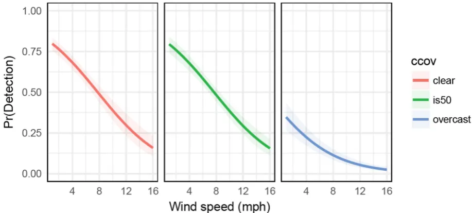
Detection probability was lowest when surveys were conducted in overcast conditions
170
(pr[detection|avg wind] = 0.11, 95% CI: 0.08 – 0.15) and were similar when the sky was clear, had less
171
than, about, and above 50% cloud cover (pr[detection|avg wind] ≈ 0.5, Figure 2). Detection
172
probability was negatively influenced by wind (βwind = -0.20, 95% CI: -0.24 – -0.16, Figure 3). For
173
example, in clear sky conditions, this effect relates to detection probability ranging from 0.80 (95%
174
CI: 0.77 – 0.83, Figure 3) when there is no wind, to 0.16 (95% CI: 0.11 – 0.23, Figure 3) when wind
175
speed is 16 mph (the highest recorded during surveys). Thus, maximum detection probability is
176
achieved when sampling in conditions where the sky is not overcast and there is no wind.
177
Our classification of whether we determined sites to be located on exposed versus sheltered
178
stretches of shoreline (exposure classification) was selected as the best model based on AIC (Table 1).
179
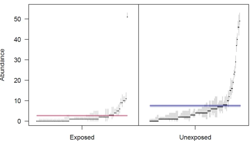
Unexposed sites had a significantly higher expected abundance than exposed sites (αexposure = 1.03,
180
95% CI: 0.85 – 1.21, estimates on the log scale). This translates to an expected abundance of 2.68 (95%
181
CI: 0.23 – 3.16, Figure 4) at exposed sites and 7.50 (95% CI: 6.87 – 8.20, Figure 4) at unexposed sites.
182
Note that the estimate of λ are the mean of the Poisson distribution, i.e., the expected value, from
183
which observed estimates of site specific abundances are assumed to be distributed. We can use the
184
count data, and estimates of detection, to estimate a ‘conditional on observation data’ abundance for
185
each site [22] (Figure 4). Local abundance at exposed sites ranged from 0 (95% CI: 0 – 1) to 51 (95%
186
CI: 51 – 53), and local abundance at unexposed sites ranged from 0 (95% CI: 0 – 1) to 106 (95% CI: 101
187
– 110). Expected and realized estimates are shown in Figure 4.
188
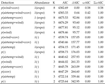
Table 1. Model selection table showing all 16 models ranked according to their AIC score (lowest is better). The
189
Detection (p) and Abundance (λ) model formulations are provided, as is the number of parameters in the model
190
(K), the AIC score, the difference in AIC relative to the top model (ΔAIC), the AIC weight (ωAIC) which is a
191
measure of relative model support, and the cumulative AIC weights (ΣωAIC).
192
Detection Abundance K AIC ΔAIC ωAIC ΣωAIC
p(wind+ccov) λ(expo) 8 4382.69 0.00 0.58 0.58
p(airtemp+wind+ccov) λ(expo) 9 4383.33 0.64 0.42 1.00 p(airtemp+ccov) λ (expo) 8 4475.53 92.84 0.00 1.00 p(airtemp+wind) λ(expo) 5 4476.29 93.60 0.00 1.00
p(ccov) λ(expo) 7 4477.81 95.12 0.00 1.00 p(wind) λ(expo) 4 4478.46 95.77 0.00 1.00
p(wind+ccov) λ(∙) 7 4539.74 157.05 0.00 1.00 p(airtemp+wind+ccov) λ(∙) 8 4540.46 157.77 0.00 1.00
p(airtemp) λ(expo) 4 4554.15 171.45 0.00 1.00 p(∙) λ(expo) 3 4558.73 176.03 0.00 1.00
p(airtemp+wind) λ(∙) 4 4640.62 257.93 0.00 1.00 p(wind) λ(∙) 3 4644.02 261.33 0.00 1.00
p(airtemp+ccov) λ(∙) 7 4645.78 263.09 0.00 1.00 p(ccov) λ(∙) 6 4647.29 264.60 0.00 1.00 p(airtemp) λ(∙) 3 4722.14 339.44 0.00 1.00
194
195
Figure 2. Per individual detection probability of diamondback terrapin heads as a function of the five cloud
196
cover categories. Estimates are reported at the lowest (1.00 mph), average (8.21 mph), and higherst (16.00 mph)
197
wind speeds recorded during the head ccunt surveys. Points are maximum likelihood estimates, and solid
198
black lines represent 95% confidence intervals.
199
200
Figure 3. Per individual detection probability of diamondback terrapin heads as a function of wind speed at
201
three (of the five) cloud cover categories. Solid lines are maximum likelihood estimates, and polygons
202
represent 95% confidence intervals.
204
Figure 4. Model estimates of expected (solid horizontal lines) and conditional (black points) estimates of
205
abundance. Expected abundance is the mean, or expected, abundance at an exposed (red line withpolygon
206
representing 95% confidence intervals) and unexposed (blue line withpolygon representing 95% confidence
207
intervals) sites. Realized abundances are assumed to be poulations sizes assumed to come from a Poisson
208
distribution with a mean λexposed/unexposed and thus vary by site. Site specific counts allow the generation of
209
realized site-specific population estimates which are conditional on the observed data. Note, that the Y-axis
210
has been truncated at 55 for enhanced visual representation of the data – there is one unexposed stite (N=106)
211
not shown here.
212
4. Discussion
213
In this study, we demonstrate how pairing visual head count surveys with N-mixture modeling
214
offers a complimentary data collection and analysis framework for efficiently estimating local
215
diamondback terrapin population sizes while simultaneously accounting for factors that affect
216
detectability and explain spatial variation in abundance. We found that, as expected, detection
217
probability was negatively influenced by wind speed and overcast skies, and our results suggest that
218
abundance was higher at sites along sheltered stretches of shoreline relative to sites that were
219
exposed. Visual head count surveys are indeed a promising and efficient method of estimating
220
abundance for this important estuarine obligate turtle.
221
Studies of DBT have been largely focused on capture mark recapture and are plagued with
222
reported issues of detectability [7,16,17]. Our study confirms that this challenge is not restricted to
223
CMR, but also impacts visual head counts. However, repeat-survey designs such as those called for
224
under the N-mixture model, are developed specifically to capture variability in imperfect counts and
225
relate that variability to variation in factors (e.g., environmental) recorded during each survey. While
226
robust design CMR is designed in the same way, an important distinction is that visual head counts
227
do not require physical capture and are designed in line with the species surfacing and aggregation
228
behavior to maximize detection, and this appears to yield far greater sample sizes. While this
229
precludes the estimation of demographic rates (survival and fecundity) that typically require
230
individual identity to be known, when the inference objective is to estimate abundance, something
231
that is lacking throughout the range, then abundance estimates from unmarked individuals as we
232
have presented here has obvious value (see Figure 4).
233
Applying the N-mixture model to repeated head count surveys, we were able to both identify,
234
and correct for, factors that influenced detectability and therefore estimate population size free of
235
these specific biases. Specifically, for DBT in Wellfleet Bay, wind reduced detectability (Figure 2) and
236
was interesting, and contrary to our expectations, that there was no substantial difference in
238
detectability with increasing cloud cover, but rather it appeared that the main difference was between
239
completely overcast and all other categories where there was at least some blue sky. This may be due
240
to the significant decrease in contrast between emergent DBT heads and the water, as both become
241
darker in color under overcast skies. The negative effect of wind on detection was expected, and likely
242
related to either increase wave chop making heads more difficult to observe or, behavior-related, that
243
DBT surface less in higher winds. While we cannot disentangle the effect of wind and cloud cover on
244
observer ability versus DBT behavioral response per se, N-mixture models do allow us to test
245
hypotheses about detectability in general. This has potential implications for other capture methods
246
that rely on visual detection of terrapins (e.g. dip netting, drones). Our study suggests that the ideal
247
conditions for conducting visual head count surveys in this system is are in low-to-no wind when it
248
is not overcast.
249
One of the most appealing features of our use of the visual head counts and N-mixture models
250
is the ability to generate estimates of population size for several, 38, locations within Wellfleet bay
251
and link those estimates to spatially varying covariates. This is in contrast with intensive CMR efforts,
252
which often require multiple seasons to generate sufficient recaptures [16,17], and have been
253
restricted to just two locations within the bay [17]. This is common throughout the range where CMR
254
estimates of abundance are typically, and justifiably, made over a spatially restricted area relative to
255
the local or regional distribution of the species [9,10]. Moreover, this improvement in the spatial
256
coverage and the statistical inference about DBT population status, at least in Wellfleet Bay, is
257
achieved far more efficiently than traditional methods [7,25], and arguably yields more
management-258
relevant results. For example, the ability to move beyond point estimates of abundance and start to
259
relate spatial variation in abundance to habitat characteristics or environmental conditions is
260
potentially far more valuable information to inform proactive species- and habitat-specific
261
conservation action.
262
Our focus here was to demonstrate the utility of visual head counts and N-mixture models as an
263
efficient method for estimating abundance, and as such, we did not exhaustively explore all potential
264
predictors of abundance. Instead, we focused on differences between sheltered and exposed
265
shorelines as a simple catch-all proxy for a wide range of environmental disturbance. As expected,
266
we found that abundances at exposed sites were on average lower than at sheltered sites. Despite
267
being a crude measure of habitat quality, these model predictions are in line with what we would
268
expect: unexposed sites experience less environmental disturbance (e.g., turbidity) where intact
269
saltmarsh habitat is more likely to be found. Also as expected, there was a great deal of variation in
270
site-specific abundances over and above the ‘exposure effect’ (Figure 4), likely reflecting unmodeled
271
spatiotemporal variation in population size arising from additional habitat preference and
272
phenologically driven changes. While not included in this effort, the next step is to focus on
273
developing a suite of potential spatiotemporal covariates to formally identity drivers of population
274
sizes in both space and time.
275
5. Conclusion
276
The visual head count methodology described here naturally matches the ecology of DBT, they
277
are easy to conduct and require very little training (i.e., low intensive), and, as demonstrated here,
278
generate spatially referenced estimates of local abundance over a large spatial extent. This contrasts
279
substantially with the widely used CMR approaches, which involve substantial effort, both in terms
280
of time and expertise (i.e., highly intensive), they often suffer from extremely low capture rates
281
requiring multiple sampling seasons to generate abundance estimates, and as a result are typically
282
limited in terms of spatial coverage. Further, we demonstrate the application of N-mixture models,
283
the canonical analytical framework for analyzing such repeated count data, and were able to identify
284
ideal survey conditions that will maximize detection in future surveys, and revealed substantial
site-285
specific variation in estimates of abundance likely due to habitat preferences and phenology. We
286
method for generating spatially explicit estimates of diamondback terrapin abundance, and drivers
288
of spatiotemporal variation in abundance that has the potential to scale up DBT population
289
assessments across their range.
290
291
Author Contributions: Conceptualization, P.L. and C.S.; methodology, P.L., C.S., S.S.; formal analysis, P.L., C.S.;
292
investigation, P.L.; writing—original draft preparation, P.L.; writing—review and editing, P.L., C.S., S.S.;
293
visualization, P.L., C.S.; supervision, C.S.; project administration, C.S., P.L.; funding acquisition, C.S., P.L..
294
Funding: This research was funded by Massachusetts Division of Fisheries and Wildlife Natural Heritage and
295
Endangered Species Program MESA mitigation funds.
296
Acknowledgments: Mike Jones (Mass Wildlife NHESP), Bob Prescott and Mark Faherty (Mass Audubon
297
Wellfleet Bay Wildlife Sanctuary) and Rachel Katz (USFWS).
298
Conflicts of Interest: The authors declare no conflict of interest.
299
References
300
[1] Hart KM, Lee DS. The diamondback terrapin: The biology, ecology, cultural history, and conservation
301
status of an obligate estuarine turtle. Stud Avian Biol 2006:206–13.
doi:10.1641/0006-302
3568(2006)56[675:TMAGPO]2.0.CO;2.
303
[2] Ernst CM, Lovich JE. Turtles of the United States and Canada. Second Edi. Baltimore: The John Hopkins
304
University Press; 2009.
305
[3] Roosenburg WM, Kennedy VS. Ecology and Conservation of the Diamond-backed Terrapin. Baltimore:
306
John Hopkins University Press; 2018.
307
[4] Harden LA, Pittman SE, Gibbons JW, Dorcas ME. Development of a rapid-assessment technique for
308
diamondback terrapin (Malaclemys terrapin) populations using head-count surveys. Appl Herpetol
309
2009;6:237–45. doi:10.1163/157075408X397527.
310
[5] Duncan NP, Burke RL. Dispersal of Newly Emerged Diamond-Backed Terrapin (Malaclemys terrapin)
311
Hatchlings at Jamaica Bay, New York. Chelonian Conserv Biol 2016;15:249–56. doi:10.2744/ccb-1207.1.
312
[6] Seigel RA. Courtship and Mating Behavior of the Diamondback Terrapin Malaclemys terrapin tequesta.
313
J Herpetol 1980;14:420–1.
314
[7] Butler JA. Population Ecology, Home Range, and Seasonal Movements of the Carolina Diamondback
315
Terrapin, Malaclemys terrapin centrata, in Northeastern Florida. Tallahassee: 2002.
316
[8] Hart KM, McIvor CC. Demography and Ecology of Mangrove Diamondback Terrapins in a Wilderness
317
Area of Everglades National Park, Florida, USA. Copeia 2008;2008:200–8. doi:10.1643/ce-06-161.
318
[9] Baxter AS, Hill EM, Withers K. Population assessment of texas diamondback terrapin 2016;65:51–63.
319
[10] Simoes JC, Chambers RM. The Diamondback Terrapins of Piermont Marsh , Hudson River , New York.
320
Northeast Nat 1999;6:241–8.
321
[11] Butler JA. Status and Distribution of the Carolina Diamondback Terrapin, Malaclemys terrapin centrata,
322
in Duval County. Tallahassee: 2000.
323
[12] Akins CD, Ruder CD, Price SJ, Harden LA, Gibbons JW, Dorcas ME. Factors affecting temperature
324
variation and habitat use in free-ranging diamondback terrapins. J Therm Biol 2014;44:63–9.
325
doi:10.1016/j.jtherbio.2014.06.008.
[13] Selman W, Baccigalopi B, Baccigalopi C. Distribution and Abundance of Diamondback Terrapins
327
(Malaclemys terrapin) in Southwestern Louisiana. Chelonian Conserv Biol 2014;13:131–9.
328
doi:10.2744/ccb-1102.1.
329
[14] Henry PFP, Haramis GM, Day DD. Evaluating a portable cylindrical bait trap to capture diamondback
330
terrapins in salt marsh. Wildl Soc Bull 2016;40:160–8. doi:10.1002/wsb.610.
331
[15] Byers JE, Altman I, Grosse AM, Huspeni TC, Maerz JC. Utilización de Larvas de Trematodos Parásitos
332
para Cuantificar a Un Hospedero Vertebrado Elusivo. Conserv Biol 2011;25:85–93.
doi:10.1111/j.1523-333
1739.2010.01583.x.
334
[16] King P, Ludlam JP. Status of Diamondback Terrapins (Malaclemys terrapin) in North Inlet–Winyah Bay,
335
South Carolina. Chelonian Conserv Biol 2014;13:119–24. doi:10.2744/ccb-1042.1.
336
[17] Mass Audubon. Wellfleet Bay Wildlife Sanctuary Diamondback Terrapins 2019.
337
[18] Ecology T, July F, Kanonik A, Rahman S, Burke R. Demographic Analysis of the Jamaica Bay
338
Diamondback Terrapin Population : Implications for Survival in an Urban Habitat. North 2010:2010–
339
2010.
340
[19] Roosenburg WM. Final Report Chesapeake Diamondback Terrapin Investigations for the Period 1987,
341
1988, and 1989. Solomons: 1990.
342
[20] Ralph CJ, Sauer JR, Droege S. Monitoring Bird Populations by Point Counts. 1995.
343
[21] Royle JA. N-Mixture Models for Estimating Population Size from Spatially Replicated Counts.
344
Biometrics 2004;60:108–15. doi:10.1111/j.0006-341X.2004.00142.x.
345
[22] Fiske IJ, Chandler RB. unmarked: An R package for fitting hierarchical models of wildlife occurrence
346
and abundance. J Stat Softw 2011;43:1–23. doi:10.1002/wics.10.
347
[23] Burnham KP, Anderson DR. Model selection and multimodel inference: a practical
information-348
theoretic approach. Springer Verlag; 2002.
349
[24] Arnold TW. Uninformative Parameters and Model Selection Using Akaike’s Information Criterion. J
350
Wildl Manage 2010;74:1175–8. doi:10.2193/2009-367.
351
[25] Selman W, Baccigalopi B, Baccigalopi C. Distribution and Abundance of Diamondback Terrapins
352
(Malaclemys terrapin) in Southwestern Louisiana. Chelonian Conserv Biol 2014;13:131–9.
353
doi:10.2744/CCB-1102.1.