Article
1
Optical micro-angiography (OMAG) based range
2
optimization method for liquid flow rate
3
Peng Chen1, Lei Jiang1, Haixia Wang1, Xiaorui Guo2, Yilong Zhang1, Yonghong He2,3,
4
and Ronghua Liang1,*
5
1 College of Information and Engineering, Zhejiang University of Technology, Hangzhou 310023, China;
6
[email protected](P.C.); [email protected](L.J.); [email protected](H.W.);
7
[email protected] (Y.Z.)
8
2 Shenzhen Key Laboratory for Minimal Invasive Medical Technologies, Institute of Optical Imaging and
9
Sensing, Graduate School at Shenzhen, Tsinghua University, Shenzhen 518055, China;
10
[email protected] (X.G.);[email protected](Y.H.)
11
3 Department of Physics, Tsinghua University, Beijing 100084, China
12
* Correspondence: [email protected]; Tel.: +86-139-5710-1740
13
14
Abstract: Optical micro-angiography (OMAG) is a new method of detecting flow rate and widely
15
used for in vivo imaging. Although OMAG can distinguish between flowing and stationary parts,
16
it cannot obtain accurate flow rate information. This study proposed a range formula for OMAG
17
and the ultrahigh-sensitivity OMAG (UHS-OMAG) method to quantify the measurement range of
18
an entire system. The parameters of the angle between beam scanning and flow directions, the
19
angular velocity of the galvanometer, and the offset of incident light were introduced, and a formula
20
for calculating the range was derived. Experiments were conducted to measure fine and ultra-fine
21
flow rates by using OMAG and UHS-OMAG methods. The minimum measured flow rate was
22
approximately 30 um/s, and the maximum measured flow rate was approximately 8 mm/s.
23
Experimental results are in good agreement with the preset results.
24
Keywords: OMAG method; flow rate measurement; micro flow rate
25
26
1. Introduction
27
Optical coherence tomography (OCT) is a rapidly emerging optical imaging technology and a
28
non-invasive imaging method [1,2] that is widely used in biology [3], medicine [4–6], and material
29
research [7,8]. Doppler OCT (DOCT) was developed by combining the Doppler principle with OCT.
30
Leigteb et al. implemented the first Fourier-domain OCT flow velocity detection experiment [9].
31
DOCT can determine the position and velocity of moving particles in high scattering media [10–12].
32
It can also be applied to microvascular in vivo imaging in medical diagnostics [13] and flow
33
characteristic measurement in microfluidic monitoring [14], which has a good application prospect.
34
However, DOCT can only measure velocity components parallel to the incident beam [15]. Therefore,
35
the incident beam angle and the flow velocity direction (Doppler angle) must be accurately
36
determined when calculating fluid velocity. However, the Doppler angle is difficult to measure in
37
many practical applications. Consequently, DOCT cannot be used successfully in practical
38
applications, especially those that involve living biological tissues.
39
To overcome these limitations, Wang et al. proposed optical micro-angiography (OMAG)
40
technology in 2007 [16] and made several improvements [17,18]. OMAG is OCT micro-angiography
41
based on complex signals. It utilizes the mathematical properties of Hilbert transform and constructs
42
complex analytical signals using the Hilbert transform of real-interference signals. The structure and
43
flow velocity information of a sample are obtained by Fourier transform. OMAG does not rely on the
44
phase information of OCT, is not sensitive to environmental noise and other factors, and has made
45
great progress in terms of the sensitivity and image quality of flow rate detection [19]. In addition to
46
its capability to achieve micro-structural imaging, OMAG provides volumetric vasculature images of
47
the scanned tissue bed down to the capillary-level imaging resolution [20]. OMAG has a high
48
application value in living microvascular imaging and has been successfully applied in human skin
49
[21], cochlea [22,23], and human retina [24,25]. The ultrahigh-sensitivity OMAG (UHS-OMAG)
50
method [26] was proposed to measure low flow velocities. This method remarkably improves
51
imaging sensitivity.
52
Although changes in sensitivity in actual flow detection can be determined using the OMAG
53
method, the method cannot effectively obtain the exact range of the system. Accurate flow rate
54
information can be obtained when small flow rates, such as capillary flow rates, are detected. This
55
information is limited in practical applications, such as medicine. For example, when measuring
56
capillary information in the human body, the flowing particles in the capillaries can be separated
57
from stationary particles, but the flow velocity information in the blood vessels cannot be accurately
58
determined.
59
In this study, we derived a range calculation formula of OMAG and UHS-OMAG for the first
60
time to quantify the system measurement range. We introduced the angle between beam scanning
61
and flow directions, the angular velocity of the galvanometer, and the offset of incident light and
62
derived a formula for calculating the range. Moreover, the images obtained within the measurement
63
range were analyzed to explore the imaging patterns within this range. Our work provides the
64
following contributions.
65
(1) After obtaining a rough estimate of the flow rate to be measured, the system’s parameter
66
values can be set according to the formula so that the measured image is displayed in the best imaging
67
area.
68
(2) When the flow rate to be measured is unknown, the approximate range of unknown flow
69
velocity can be calculated based on the measured image and parameter values of the system.
70
In our experiments, we estimated the flow rate by using our derived range formula, and the
71
experimental results were consistent with the predicted results. We also analyzed the relationship
72
between the intensity value of the obtained experimental result image and flow rate. A linear
73
relationship was established between the intensity value of the image and flow velocity within the
74
range.
75
2. System and theory analysis
76
2.1. System setup
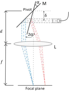
77
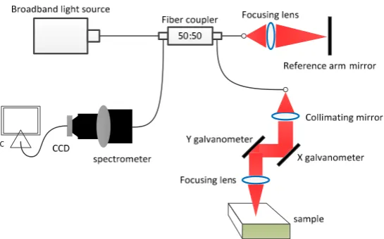
The system used in this experiment is shown in Figure 1. The system consists of a
78
superluminescent diode (SLD) as the light source with a center wavelength of 1310 nm and a
79
bandwidth of 75 nm. The theoretical longitudinal resolution determined by the light source is 10 um.
80
The light from the source is split into two paths through a 50:50 2×2 optocoupler. One light path is
81
directed at a mirror called the reference arm, and the other light path is directed through the sample
82
arm directly toward the sample. The light in the sample arm is coupled into an optical system that
83
includes a collimator, a pair of X- and Y-axis galvanometers, and a 50 mm focal length objective with
84
a theoretical lateral resolution of 17 um. The beam is reflected from the reference arm, and the sample
85
arm is subsequently coupled into the detection arm and transmitted to a high-speed spectrometer to
86
detect spectral interference signals. SENSORS’ GL2048R linear array charge-coupled device (CCD)
87
was the spectrometer used in this study. The number of pixels is 2048, the single pixel size is 10 um
88
× 210 um, and the maximum sampling frequency is up to 147 kHz. The galvanometer imaging speed
89
in our system is 600 mm/s, and the galvanometer reset speed is 3000 mm/s. The sampling frequency
90
of the CCD and the scanning length can be changed in the program to modify the scanning frequency
91
of the B scanning direction and the galvanometer speed of the Y galvanometer.
93
Figure 1. Schematic of the OMAG system used in this study.
94
2.2. Theory
95
The core concept of the OMAG method is to construct a complex analytical signal by using the
96
Hilbert transform of the real-interference signal and obtain the structure and flow rate information
97
of the sample by Fourier transform. Hilbert transform rotates the phase of a signal counterclockwise
98
by 90°. We subsequently constructed an analytical signal whose imaginary part is the Hilbert
99
transform of the real part. Then, we obtained structure and flow rate information in the signal by
100
performing Fourier transform on the obtained analytical signal. Figure 2 shows that Hilbert and
101
Fourier transform need to be performed in X and K directions, respectively, whereas traditional OCT
102
can conduct Fourier transform directly in the K direction.
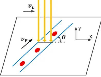
103
104
Figure 2. OMAG flow chart.
105
We can regard the 2D raw data obtained by OCT as a 2D array. The horizontal axis is time t, and
106
the vertical axis is wave number k. We used a function with two variables to represent
107
( )
,
cos 2
02
(
C D)
B k t
=
kz
+
π
f
−
f t
+
φ
, (1)108
where 𝑧 is the initial depth position of the reflective particles at lateral position x and ∅ is a
109
random phase term. 𝑓 is the modulation frequency component, and 𝑓 is the Doppler frequency
110
component. Variables t and k are irrelevant, that is, when t changes, k is constant and vice versa.
111
When the modulation frequency 𝑓 − 𝑓 does not overlap with the signal bandwidth introduced by
112
the random phase term, we can construct the analytic function of t by using the Hilbert transform
113
constructor (1) based on the Bedrosian theorem [27]. In this case, the Hilbert transform of Equation
(1) is equal to its orthogonal representation, and 2𝑘𝑧 is currently a constant phase term. If 𝑓 − 𝑓 >
115
0, then the analytic function of Equation (1) is
116
( )
,
cos 2
(
C D)
2
0sin 2
(
C D)
2
0H k t
=
π
f
−
f t
+
kz
+ +
φ
j
π
f
−
f t
+
kz
+
φ
. (2)117
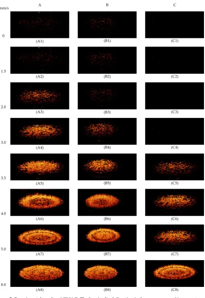
If 𝑓 − 𝑓 < 0, then the analytic function of Equation (1) is
118
( )
,
cos 2
(
C D)
2
0sin 2
(
C D)
2
0H k t
=
π
f
−
f t
+
kz
+ −
φ
j
π
f
−
f t
+
kz
+
φ
. (3)119
Mathematically, Equation (3) is a complex conjugate form of Equation (2). We performed Fourier
120
transform with k as the argument, where t is a constant term. The frequency component 𝑧 of
121
Equation (2) is located in the positive space of the entire Fourier domain, and the frequency
122
component of Equation (3) is located in the negative space of the Fourier domain. This part is the
123
most critical in the OMAG approach.
124
The derivation shows that a fixed carrier frequency must be introduced to satisfy Hilbert
125
transform and obtain a quadrature signal. The introduction of carrier frequency aims to add one item
126
to the phase term of the interference signal, that is, a phase change occurs, and the phase change is
127
the change in the optical path difference. Thus, the introduction of the fixed carrier frequency
128
essentially causes the optical path difference to exhibit variety. This objective can be achieved by
129
using two methods, namely, piezoelectric and offset. In the piezoelectric method, the piezoelectric
130
ceramic drives the reference arm mirror to move at a uniform speed to introduce a carrier frequency.
131
The offset method aims to make the collimating light of the sample arm deviate from the rotation
132
center of the galvanometer to change the optical path and introduce a fixed carrier frequency.
133
The hardware of the piezoelectric OMAG method is different from that of a conventional
134
frequency-domain OCT device. A piezoceramic needs to be installed on the reference arm mirror to
135
drive the reference arm mirror to move at a constant speed and thus introduce a fixed frequency shift.
136
We assumed that the reference mirror moves at a speed of 𝑣 , and the velocity of the moving
137
particles in the direction of the probe beam is 𝑣. At this point, we can express the interferogram of
138
the spectrum as
139
( )
,
cos 2
{
0(
ref s)
}
B k t
=
k z
+
v
−
v t
+
φ
. (4)140
Equation (4) shows that when 𝑣 − 𝑣 > 0, the region is imaged in the positive space. When
141
𝑣 − 𝑣 < 0, the region is imaged in the negative space, and moving and static particles are
142
separated.
143
The offset OMAG method introduces a fixed carrier frequency in such a way that the sample
144
arm collimates light away from the center of the galvanometer. Compared with the piezoelectric
145
method, the offset method does not require a single chip microcomputer or a driving circuit, and the
146
entire system is simpler. Moreover, the piezoelectric method always moves while the reference arm
147
mirror is moving during the scanning process. Thus, the spectrum of the returning light of the
148
reference arm is constantly shaking, leading to additional noise in the resulting image. The offset
149
method can also increase the imaging speed without adding a control module and without affecting
150
the effect.
151
A schematic of the offset OMAG method is shown in Figure 3. In conventional
frequency-152
domain OCT, the sample arm’s collimated light is usually located at an angle of 45° relative to the
153
initial galvanometer. We assumed that the optical path difference between the reference and sample
154
arms is zero. The incident light subsequently moves downward by a distance of δ so that the incident
155
light deviates from the rotation center of the galvanometer. After the incident light is reflected by
156
galvanometer M, it is focused by objective lens L onto the focal plane. The focal length of the objective
157
lens L is 𝑓, the distance between the rotation center of the galvanometer and the objective lens is d,
158
and the rotation angle of galvanometer M relative to the initial position is α. The change in the optical
159
path of the galvanometer during lateral scanning can be calculated by ray tracing as follows [28]:
160
( )
(
( )
)
sin
1
1
2
cos 2
sin 45
OPD
d
α
α
α
°α
=
− +
−
. (5)
δ α
2α
𝑓 𝑑
162
Figure 3. Schematic of the beam offset method at the sample arm.
163
3. Range derivation
164
Our derivation began with the piezoelectric OMAG method because the minimum
165
measurement of piezoelectric OMAG is readily available. Then, a range calculation formula of the
166
offset method was derived according to the relationship between the piezoelectric and offset OMAG
167
methods. We also derived a range calculation formula of UHS-OMAG.
168
3.1. Derivation process
169
We generally have uneven high-scattering samples when detecting targets. Hence, the random
170
phase term ∅ in Equation (1) varies randomly with time −𝜋,𝜋 . The frequency component of ∅
171
with respect to t is a function of random distribution around zero frequency, and its bandwidth is
172
BW. The envelope of this spectral distribution depends on the correlation between the interference
173
signals at different positions of the sample. The bandwidth BW of this envelope is also limited by the
174
sampling frequency 𝑓 of the system. If BW and 𝑓 are very close, then almost no correlation exists
175
between the interference signals at different positions of the sample. We introduced modulation
176
frequency 𝑓 to obtain the analytical signal and subsequently remove its frequency band from the
177
zero-frequency region until no overlap exists between the frequency band of the parsing signal and
178
its complex conjugate frequency band. For its Hilbert transform to be strictly equal to its orthogonal
179
form, the spectrum that corresponds to the phase term that changes over time is shifted to a position
180
where no overlap with the zero frequency exists. We obtained the applicable conditions of the OMAG
181
algorithm as follows:
182
2
cBW
f
>
. (6)183
BW determines the minimum speed that the system can detect. The smaller BW is, the smaller
184
the value of 𝑓 is and the lower the equivalent threshold speed is; hence, a small flow rate can be
185
detected. In our derivation, the condition of BW < 2 𝑓 was always met.
186
The optical path difference (OPD) at this time in the piezoelectric OMAG method is the distance
187
𝑣 𝑡 of the reference arm motion, the phase change is 2𝑘𝑣 𝑡, and the modulation frequency is
188
2𝑘 𝑣 − 𝑣 , that is, the introduced carrier frequency 𝑓 is 𝑘𝑣 / 𝜋. Notably, 𝑣 and 𝑣 in
189
Equation (4) are vector representations. Relative to the movement of the reference mirror, the
190
opposite movement of the particles reduces the difference in optical path length between the sample
191
and reference arm and decreases the effective frequency of the modulation. When the value of 𝑣 is
192
sufficiently large, the moving particles are projected onto the positive space. In general, when the
193
reference arm mirror moves toward the fiber coupler at speed 𝑣 , it is equivalent to the sample arm
that moves toward the galvanometer at velocity 𝑣 . At this time, only velocity 𝑣 moves upward,
195
and the particles of 𝑣 > 𝑣 are imaged on the dynamic plane. The same condition applies when
196
the reference arm mirror moves in a direction opposite to the fiber coupler. Evidently, the minimum
197
moving particle that can be measured by the piezoelectric OMAG method is greater than 𝑣 . In
198
summary, we can obtain the lowest actual speed as follows:
199
min
cos
ref
v
v
θ
=
. (7)200
In our work, the angle 𝜃 between beam scanning and flow directions was introduced for the
201
first time to the range calculation of OMAG and UHS-OMAG. Notably, this θ is not the angle between
202
the incident beam and the direction of flow velocity. Figure 4 shows that 𝑣 is the scanning direction
203
of the beam, 𝑣 is the moving direction of the particles, and θ is the angle between 𝑣 and 𝑣 .
204
𝜽
𝒗
𝑳𝒗
𝑭205
Figure 4. Schematic of the angle θ between the scanning direction of the beam and the direction of
206
flow velocity.
207
In the conventional OMAG method, the phase difference between adjacent A lines in the B-scan
208
is used to estimate flow velocity. Thus, the velocity during measurement is a component of 𝑣 in X
209
direction, and the measured velocity is 𝑣 cos 𝜃. In UHS-OMAG, the A-line density in B-scan is
210
reduced, the scanning density of B-scan is increased, and the OMAG algorithm is applied to the
C-211
scan direction. Therefore, the measured speed is 𝑣 . A component of the Y direction, the measured
212
velocity is 𝑣 sin 𝜃.
213
In the offset OMAG method, as indicated in Equation (5), α is small when our system collects
214
data, and the first term in the equation is negligible compared with the second term when making
215
phase changes. Thus, the phase change of the interference signal can be approximated as
216
4
k
4
k
t
ϕ
=
αδ
=
δω
. (8)217
where ω is the angular velocity of the X galvanometer and t is the scan time. Through the phase
218
change, the change in the OPD of the offset method and the introduced carrier frequency value can
219
be obtained, as shown in Table 1.
220
Table 1. Comparison of piezoelectric and offset methods.
221
Piezoelectric method Offset method
Optical path difference (𝑂𝑃𝐷) 𝑣 𝑡 2𝛿𝜔𝑡 Phase change (φ) 2𝑘𝑣 𝑡 4𝑘𝛿𝜔𝑡 Introducing carrier frequency (𝑓) 𝑘𝑣 / 𝜋 2𝑘𝛿𝜔/𝜋
222
A comparison of the two methods showed that the minimum speed that can be measured with
223
the piezoelectric method is the velocity of the reference arm mirror 𝑣 , which can be obtained via
224
conversion using the offset method as follows:
225
min
2
cos
cos
ref
v
v
δω
θ
θ
=
=
. (9)The maximum detection speed of the system is determined by the sampling frequency.
227
According to the sampling theorem, the sampling frequency should be greater than twice the highest
228
frequency component of the signal. Sampling frequency refers to time sampling, which is the
229
sampling frequency 𝑓 of the CCD. In summary, the range of an ordinary OMAG system is
230
max
4 cos
reqv
f
λ
θ
=
. (10)231
3.2. UHS-OMAG range
232
Equation (9) shows that measuring a low flow velocity requires reducing BW and the
233
galvanometer speed to obtain high sensitivity. However, BW cannot be reduced by reducing the
234
diameter of the collimated light because the light source of our system is deterministic, and the effect
235
of this method is limited. Thus, the speed of the galvanometer must be reduced to improve sensitivity.
236
However, as the galvanometer speed decreases, the overall imaging process time increases
237
considerably, thereby affecting the final image quality. Moreover, this method cannot achieve a
238
remarkable increase in sensitivity, so the highly sensitive UHS-OMAG method was proposed. In
239
contrast to the conventional OMAG method, UHS-OMAG reduces the density of A lines in the
B-240
scan, increases the scanning density of the B-scan, and applies the ordinary OMAG algorithm to the
241
C-scan direction. In the actual measurement process, ordinary OMAG only needs to complete a 2D
242
scan, and the Hilbert transform structure analysis signal is implemented in the B-scan direction.
UHS-243
OMAG must complete a 3D scan once and take an A line from each B-scan to form a 2D map.
244
Subsequently, a Hilbert transform structure analysis signal is created for this 2D map. When using
245
the offset method, the beam at this time needs to deviate from the rotation center of the Y
246
galvanometer and not that of the X galvanometer.
247
Attention should be paid to the changes in range calculation when using the UHS-OMAG
248
method. Compared with Equation (9), ω is no longer the angular velocity of the X galvanometer at
249
this time. Instead, it is the angular velocity 𝜔 of the Y galvanometer, δ is the distance 𝛿 of the
250
rotation center of the offset Y galvanometer, and 𝑓 in Equation (10) is no longer the sampling
251
frequency of the CCD but the scanning frequency 𝑓 of B. The influence of angle θ between the beam
252
scanning and flow velocity directions in the UHS-OMAG method should be given attention. In
253
summary, the range of the UHS-OMAG method is
254
min
2
sin
Y Y
v
δ ω
θ
=
, (11)255
max
4sin
Bv
f
λ
θ
=
. (12)256
4. Results and discussion
257
We used the offset method in the experiment. A capillary tube with an inner diameter of 0.4 mm
258
was utilized as a channel, and milk was employed as a test fluid. A constant flow pump was used to
259
provide a known steady flow rate.
260
From the system in Figure 1, we acquired spectral interference raw data from which the OMAG
261
signal was calculated. We only needed a B-scan to process in the OMAG algorithm. In the 3D data
262
block obtained by the acquisition system, we took Hilbert and Fourier transform from the acquired
263
B-scan to complete the OMAG imaging. We obtained the spectral data matrix row by row to derive
264
the analysis function using Hilbert transform. Then, we performed Fourier transform on the data
265
matrix of Hilbert transform column by column. We divided the frequency components into positive
266
and negative spaces of the Fourier domain. The flow partial region was imaged on a positive plane,
267
and the stationary partial region was imaged on a negative plane. Positive plane imaging minus
268
negative plane imaging resulted in an OMAG image.
269
4.1. OMAG range verification
(A1)
(A2)
(A3)
(A4)
(A5)
(A6)
(A7)
(A8)
(B1)
(B2)
(B3)
(B4)
(B5)
(B6)
(B7)
(B8) (C8)
(C7) (C6) (C5) (C1)
(C2)
(C3)
(C4)
A B C
0
1.5
2.0
3.0
3.5
4.0
5.0
8.0 mm/s
271
Figure 5. Experimental results of OMAG. The longitudinal direction is the same group of images at
272
different flow rates, with the flow rate being gradually increased; the lateral direction is the
273
experimental image of different groups at the same flow rate.
274
We divided our OMAG experiment into groups A, B, and C. In the group A experiment, our
B-275
scan direction length was set to 3 mm, the CCD sampling frequency 𝑓 was 12 KHz, the scanning
276
density was 500 lines/mm, the offset δ was 2.5 mm, and the galvanometer angular velocity was 24
277
mm/s. In the group B experiment, we did not change the other parameters, we reduced the scanning
278
density to 200 lines/mm, and the galvanometer angular velocity was increased to 60 mm/s. In the
279
group C experiment, the other parameters were unchanged compared with those in group A. The
CCD sampling frequency 𝑓 was increased to 24 KHz. We compared the variation in the range of
281
angular velocity of the galvanometer based on the results of groups A and B. By comparing groups
282
A and C, we determined the range when the CCD sampling frequency changed.
283
According to the parameters of our experimental system, the theoretical ranges of the three sets
284
of experiments were calculated using Equations (9) and (10), as shown in Table 2.
285
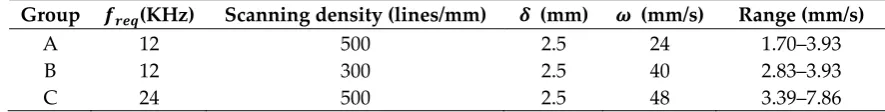
Table 2. OMAG experimental parameter settings.
286
Group 𝒇𝒓𝒆𝒒(KHz) Scanning density (lines/mm) 𝜹 (mm) 𝝎 (mm/s) Range (mm/s)
A 12 500 2.5 24 1.70–3.93
B 12 300 2.5 40 2.83–3.93
C 24 500 2.5 48 3.39–7.86
287
The pseudo color image results obtained through our experiments are shown in Figure 5, in
288
which the leftmost side is the flow rate in mm/s.
289
The experimental results show that several images, such as A1 and A2 in group A; B1, B2, and
290
B3 in group B; and C1, C2, C3, and C4 in group C, were not removed due to unavoidable slight jitter.
291
Particles with an effective velocity were not screened out because their velocity was lower than the
292
measurement range. In such a case, the imaging in each group was the same because the imaging
293
images of A1 and A2 were the same.
294
As the speed increased, the particles that entered the range of the speed range were screened
295
out. In the beginning, the velocity of the central portion of the test tube was higher than that of the
296
wall portion, which conforms to the physical law. As the speed increased, many other particles
297
entered the speed range, and the particles around the tube wall were also displayed. After the speed
298
exceeded the range, some of the particles outside of this range were imaged onto the velocity plane,
299
and some were imaged on the static plane. Phase winding occurred, and a circular pattern was
300
created. In group A, the imaging at a flow rate of 2 mm/s was A3, at which point moving particles in
301
the center of the test tube were already observed. As the flow rate and brightness increased, phase
302
winding began to occur when the image was A6, and the measurable range was exceeded. In group
303
B, when imaging B4 was just entering the range, imaging B6 was just beyond the range. In group C,
304
when imaging C5 was just entering the range, imaging C8 was just beyond the range. The
305
experimental results show that the detectable flow rates of groups A, B, and C were 1.7 to 3.9, 2.8 to
306
3.9, and 3.4 to 7.9 mm/s, respectively. This result is consistent with the range we calculated using the
307
formula.
308
4.2. UHS-OMAG range verification
309
The UHS-OMAG experiment was performed differently in comparison with the ordinary
310
OMAG method. UHS-OMAG requires a C-scan image in a 3D data block. We took all B-scan images,
311
composed a 3D data block, and took a C-scan image from the block. To complete this process, we
312
took out the A line of the same position of each B-scan in MATLAB and formed a C-scan image. Then,
313
we processed the 2D spectrum of the reconstructed C-scan image and performed the same Hilbert
314
and Fourier transform and subsequent processing as those in ordinary OMAG.
315
We divided our UHS-OMAG experiment into groups D, E, and F. In the group D experiment,
316
the CCD sampling frequency was 60 kHz, the scanning density was 60 lines/mm, the B scanning
317
direction length was 1 mm, the C scanning direction scanning density was 600 lines/mm, offset 𝛿
318
was 2.5 mm, and the scanning length was 2 mm.
319
In the group E experiment, we only changed the length of the B-scan direction (set it to 2 mm).
320
A change in the length of the B-scan direction would change the B-scan frequency and the speed of
321
the Y galvanometer. In the group F experiment, we continued to increase the length of the B-scan
322
direction and observed the change in the range.
323
The theoretical ranges for the three sets of experiments were calculated with Equations (11) and
324
(12). In accordance with our system parameters, we obtained B-scan frequency (𝑓 ) and Y-magnitude
325
speed (𝜔 ) (Table 3).
Table 3. UHS-OMAG experimental parameter settings.
327
Group B-scan length(mm) 𝒇𝑩(Hz) 𝜹𝒀(mm) 𝝎𝒀(mm/s) Range (um/s)
D 1 750 2.5 1.250 85–347 E 2 375 2.5 0.625 44–174 F 3 250 2.5 0.417 29–116
328
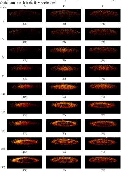
The pseudo color image results obtained through our experiments are shown in Figure 6, in
329
which the leftmost side is the flow rate in um/s.
330
D E F
(D1)
(D2)
(D3)
(D4)
(D5)
(D6)
(D7)
(D8)
(D9)
(E1)
(E2)
(E3)
(E4)
(E5)
(E6)
(E7)
(E8)
(E9) (F9)
(F8) (F7) (F6) (F5) (F4) (F3) (F1)
(F2) 0
30
50
90
120
180
240
350
500 um/s
331
A comparison of images D1, F1, and E1 with A1, B1, and C1 showed that the mirror image that
333
was not eliminated was more significant in the same state of 0 flow rate because the UHS-OAG
334
method acquired more effects due to subtle jitter.
335
The same analysis was applied to group D. When imaging D4 was just entering the range,
336
imaging D8 began to phase entangle beyond the range. In group E, when imaging E3 was just
337
entering the range, imaging E6 began to phase entangle beyond the range. In group F, when imaging
338
F4 was just entering the range, imaging F6 was just beyond the range. Our experimental results
339
showed the flow rates detected by groups D, E, and F were 90 to 350, 50 to 180, and 30 to 120 um/s,
340
respectively, which are consistent with the theoretical calculation range values in Table 3.
341
We processed all the collected data by using the UHS-OMAG method. The relationship between
342
the average light intensity value and the flow rate of the obtained experimental image is shown in
343
Figure 7.
344
345
Figure 7. Relationship between average light intensity values and flow rate in the UHS-OMAG
346
method.
347
When the flow rate was small, the jitter effect was not eliminated in all three cases; the higher
348
sensitivity was, the greater the group influence was. In the range, the average light intensity value
349
gradually increased as the flow rate increased. Beyond the range was exceeded, phase winding began
350
to occur, and the average light intensity value began to fluctuate. Within the range, the intensity value
351
of the imaged image was linear to the magnitude of the flow velocity.
352
5. Conclusions
353
We developed a flow rate range calculation formula for the common OMAG method and
high-354
sensitivity UHS-OMAG method to quantify system sensitivity. We analyzed the piezoelectric OMAG
355
method and the offset OMAG method. We used the variation in OPD and introduced the angle θ
356
between beam scanning and flow velocity directions to accurately calculate the range under the
357
OMAG method. The calculated range can be applied to normal OMAG flow rate detection and in the
358
more sensitive UHS-OMAG method. We also obtained a linear relationship between the intensity
359
value of the experimental image obtained under the OMAG method and the flow rate in the range
360
by analyzing the experimental image. Our work is of considerable value in the practical application
361
of the OMAG methodology in the future.
362
Author Contributions: conceptualization, P.C. H.W. and Y.H.; methodology, L.J., X.G. and Y.H.; software, X.G.;
363
validation, L.J., X.G. and Y.Z.; formal analysis, L.J. and Y.Z.; investigation, P.C. and L.J.; resources, P.C.; data
364
curation, X.G. and L.J.; writing—original draft preparation, L.J.; writing—review and editing, P.C, L.J. and H.W.;
365
Funding: This research was funded by the National Natural Science Foundation of China (NSFC), grant number
367
61527808.
368
Conflicts of Interest: The authors declare no conflict of interest.
369
References
370
1. Fercher, A.F.; Drexler, W.; Hitzenberger, C.K.; Lasser, T. Optical coherence tomography-principles and
371
applications. Rep. Prog. Phys. 2003, 66. 239-303.
372
2. Tomlins, P.H.; Wang, R.K. Theory, development and applications of optical coherence tomography. Journal
373
of Physics D Applied Physics.2005, 38, 2519-2535.
374
3. Ravichandran, N.K.; Wijesinghe, R.E.; Lee, S.Y.; Choi, K.S.; Jeon, M.Non-Destructive Analysis of the
375
Internal Anatomical Structures of Mosquito Specimens Using Optical Coherence Tomography. Sensors.
376
2017, 17, 1897.
377
4. Tsai, M.T.; Tsai, T.Y.; Shen, S.C.; Ng, C.; Lee, Y.J. Evaluation of Laser-Assisted Trans-Nail Drug Delivery
378
with Optical Coherence Tomography. Sensors. 2016, 16, 2111.
379
5. Jansen, S.M.; Almasian, M.; Wilk, L.S. Feasibility of Optical Coherence Tomography (OCT) for
Intra-380
Operative Detection of Blood Flow during Gastric Tube Reconstruction. Sensors. 2018, 18.
381
6. Dimitrova, G.; Chihara, E.; Takahashi, H.; Amano, H.; Okazaki, K. AuthorResponse: Quantitative Retinal
382
Optical Coherence Tomography Angiographyin Patients With Diabetes Without Diabetic Retinopathy.
383
Investigative Ophthalmology & Visual Science. 2017, 58, 190.
384
7. Shirazi, M.F.; Park, K.; Wijesinghe, R.E.; Jeong, H.; Han, S. Fast Industrial Inspection of Optical Thin Film
385
Using Optical Coherence Tomography. Sensors. 2016, 16.
386
8. Shirazi, M,F.; Jeon, M.; Kim, J. Structural Analysis of Polymer Composites Using Spectral Domain Optical
387
Coherence Tomography. Sensors. 2017, 17.
388
9. Leitgeb, L.; Schmetterer, W.; Drexler, A.; Fercher, R.; Zawadzki, T.; Bajraszewski. Real-time assessment of
389
retinal blood flow with ultrafast acquisition by color Doppler Fourier domain optical coherence
390
tomography. Optics Express. 2003, 11, 3116-3121.
391
10. Wang, X.J.; Milner, T.E.; Nelson, J.S. Fluid flow velocity characterization by optical Doppler tomography.
392
Optics Letters. 1995, 20, 1337-1339.
393
11. Chen, Z.; Milner, T.E.; Dave, D.; Nelson, J.S. Optical Doppler tomographic imaging of fluid flow velocity
394
in highly scattering media. Optics Letters. 1997, 22, 64-66.
395
12. Izatt, J.A.; Kulkarni, M.D.; Yazdanfar, S.; Barton, J.K.; Welch, A.J. In vivo Doppler flow imaging of picoliter
396
blood volumes using optical coherence tomography. Optics Letters. 1997, 22, 1439-1441.
397
13. Bonesi, M.; Matcher, S.; Meglinski, I. Doppler optical coherence tomography in cardiovascular applications.
398
Laser Physics. 2010, 20, 1491-1499.
399
14. Veksler, B.; Kobzev, E.; Bonesi, M.; Meglinski, I. Application of optical coherence tomography for imaging
400
of scaffold structure and micro-flows characterization. Laser Physics Letters. 2010, 5, 236-239.
401
15. Ahn, Y.C.; Jung, W.; Chen, Z. Quantification of a three-dimensional velocity vector using spectral-domain
402
Doppler optical coherence tomography. Optics Letters. 2007, 32, 1587-1589.
403
16. Wang, R.K.; Jacques, S.L.; Ma, Z.; Hurst, S.; Hanson, S.R. Three dimensional optical angiography. Optics
404
Express. 2007, 15, 4083-4097.
405
17. Wang, R.K. Optical Micro angiography: A Label-Free 3-D Imaging Technology to Visualize and Quantify
406
Blood Circulations Within Tissue Beds In Vivo. IEEE Journal of Selected Topics in Quantum Electronics. 2010,
407
16, 545.
408
18. Wang, R.K.; An, L.; Saunders, S.; Wilson, D.J. Optical microangiography provides depth-resolved images
409
of directional ocular blood perfusion in posterior eye segment. Journal of Biomedical Optics. 2010, 15, 020502.
410
19. Wang, R.K.; Hurst, S. Mapping of cerebro-vascular blood perfusion in mice with skin and skull intact by
411
optical micro-angiography at 1.3 mum wavelength. Optics Express. 2007, 15, 11402-11412.
412
20. An, L.; Wang, R.K. In vivo volumetric imaging of vascular perfusion within human retina and choroids
413
with optical micro-angiography. Optics Express. 2008, 16, 11438-11452.
414
21. Baran, H.; Li, L.; Choi, W.J.; Kalkan, G.; Wang, R.K. High resolution imaging of acne lesion development
415
and scarring in human facial skin using OCT-based microangiography. Lasers in Surgery & Medicine. 2015,
416
22. Choudhury, N.; Chen, F.; Shi, X.; Nuttall, A.L.; Wang, R.K. Volumetric Imaging of Blood Flow within
418
Cochlea in Gerbil in vivo. IEEE journal of selected topics in quantum electronics: a publication of the IEEE Lasers
419
and Electro-optics Society. 2009, 99, 1-6.
420
23. Subhash, H.M.; Davila, V.; Sun, H.; Nguyenhuynh, A.T.; Shi, X. Volumetric in vivo imaging of
421
microvascular perfusion within the intact cochlea in mice using ultra-high sensitive optical
422
microangiography. IEEE Trans Med Imaging. 2011, 30, 224-230.
423
24. Liu, L.; Jia, Y.; Takusagawa, H.L.; Pechauer, A.D.; Edmunds, B. Optical Coherence Tomography
424
Angiography of the Peripapillary Retina in Glaucoma. Jama Ophthalmol. 2015, 133, 1045-1052.
425
25. Campbell, J.P.; Zhang, M.; Hwang, T.S.; Bailey, S.T.; Wilson, D.J. Detailed Vascular Anatomy of the Human
426
Retina by Projection-Resolved Optical Coherence Tomography Angiography. Scientific Reports. 2017, 7,
427
42201.
428
26. An, L.; Qin, L.; Wang, R.K. Ultrahigh sensitive optical micro angiography for in vivo imaging of
429
microcirculations within human skin tissue beds. Optics Express. 2010, 18, 8220-8228.
430
27. Bedrosian, E. A product theorem for Hilbert transforms. Proceedings of the IEEE, 2005, 51, 868-869.
431
28. Wang, R.K. Use of a scanner to modulate spatial interferograms for in vivo full-range Fourier-domain