Article
A Violently Tornadic Supercell Thunderstorm
Simulation Spanning a Quarter-Trillion Grid
Volumes: Computational Challenges, 1/0
Framework, and Visualizations of Tornadogenesis
Leigh Or£ 1
G
2
3 4 s e
1
8
g
10 11
12
13
14
1 The Cooperative Institute for Meteorological Satellite Studies (CIMSS), University of Wisconsin - Madison;
leigh.orf@ssec. wisc.ed u
Abstract: Tornadoes remain an active subject of observational and numerical research due to the damage and fatalities they cause worldwide as well as poor understanding of their behavior, such as what processes result in their genesis and what determines their longevity and morphology. A numerical model executed on a supercomputer run at high resolution can serve as a powerful tool for exploring the rapidly evolving tornado-scale features within a simulated storm, but saving large amounts data for meaningful analysis can result in unacceptably slow model performance, an unwieldy amount of saved data, and saved data spread across millions of files. In this paper, a system for efficiently saving and managing hundreds of terabytes of compressed model output is described in order to support a supercomputer simulation of a tornadic supercell thunderstorm. The challenges of managing a simulation spanning over a quarter trillion grid volumes across the Blue Waters supercomputer are also described. The simulated supercell produces a long-track EFS tornado, and the near-tornado environment is described during tomadogenesis, where single upward-growing vortex undergoes several vortex mergers before transitioning into a multiple vortex tornado.
Keywords: Tornadogenesis; numerical simulation; volume rendering; visualization; supercell
u thunderstorm; Hierarchical Data Format; ZFP compression; VAPOR3
10 1. Introduction
11 Supercell thunderstorms remain an active target of both observational and numerical study, as 18 they are the source of the majority of observed tornadoes, and are always associated with the most 1g damaging, those rated EF4 and EFS on the Enhanced Fujita scale. Since the 1970s, when computing 20 technology had advanced enough, numerical models have been used to explore the three-dimensional 21 structure and morphology of supercell thunderstorms. The earliest simulations (e.g., [1-3]) were 22 coarsely resolved and spanned a domain too small to hold the full storm, which limited their utility; 23 however these same simulations captured important physical and morphological characteristics of 24 supercells that have been found to be consistent with both theory and observations. Since this time, 2s additional 3D cloud model simulations, e.g., [4-13], containing tornadoes or tornado-like vortices 20 have been conducted at increasingly higher resolutions over time; however it is not clear that data is 21 being saved at high enough spatial and temporal resolution to capture the relevant processes involving 28 tornado genesis and maintenance in many of these simulations.
2g Despite advances in computing technology and numerical model sophistication, adequately 30 resolved simulations of tornado producing supercells are lacking. Observational and numerical studies 31 of tornado producing supercells have shown an abundance of subtornadic vortices along cold pool 32 boundaries in supercells [14-17]. The smallest of these vortices exhibit diameters of tens of meters, and
33 hence could not be present in supercell simulations run with 0(100) meter resolution found in many 34 recent studies, nor would even the most sophisticated subgrid turbulence closure be able to account
35 for these unresolved features. Further, many numerical studies of supercells use a stretched mesh 36 focusing the most vertical resolution at the ground but decreasing with height. This configuration can
37 result in improperly dissipating turbulent kinetic energy, piling up energy at high wave numbers [18]. 38 These choices of problem size and the use of a stretched mesh are chosen pragmatically to make the 39 simulation less computationally intensive. While most, but not all, modern thunderstorm models
40 are able to take advantage of distributed memory architectures such as those found on modern
41 supercomputing hardware, scaling a simulation to run efficiently on hundreds of thousands to millions
42 of processing cores is a nontrivial exercise. Without special attention to the underlying communication 43 infrastructure, numerical models will scale poorly to large core counts to make such high resolution 44 simulations unfeasible. In the United States, federally funded supercomputing systems such as Blue
45 Waters [19,20] require a full NSF proposal process that includes evidence of reasonable scaling to large
46 core counts. A model that scales poorly will likely not be granted access to run at large core counts,
47 and even if it was, the amount of useful science produced would be minimal.
48 Further limiting scientists' ability to run large simulations on distributed memory supercomputers
40 is the input/output (I/O) bottleneck. Typically, simulations of supercells are executed whereby
60 floating-point data is saved periodically (typically on the order of once per model minute or more)
51 for post hoc analysis, which can take many months to years to complete due to the complexity 62 of the simulation and the traditional methods for doing analysis (such as the use of Lagrangian 53 tracers). A recent trend in large-scale modeling is the use of in situ visualization and analysis [21] s4 which enables investigators to visualize model output (and even manipulate the simulation) on
ss the same supercomputing resources while the model's state is held in core memory. The utility of
56 in situ visualization and analysis for tornado research is questionable, however, considering that a
57 scientifically interesting simulation may take months to years to analyze, and this analysis will be done
58 from files saved to disk that are repeatedly accessed with analysis and visualization software, much of s• which may be written by investigators long after the simulation was executed. This typical analysis
60 workflow does not benefit from the ability to visualize and/ or analyze a simulation while it is in core
61 memory of a supercomputer.
62 Thus, a significant limiting factor in conducting research on tornadic supercells is the ability to 63 save significant amounts of data frequently in order to capture, at high resolution, the rapidly evolving
64 flow associated with tornado behavior. Abundant visual evidence and radar observations indicate that 65 the process of tornadogenesis often occurs rapidly, over periods of dozens of seconds, where surface 66 flow quickly goes from nontornadic to producing visible debris from tornado strength damage. These
67 observations further support the notion that in order to properly model tornado behavior in supercells,
68 a small time step (associated with a small grid spacing) is required.
60 The well-known issue with increasing resolution in a three-dimensional model is that halving 70 the grid spacing (doubling the resolution) requires 23 (8) times more computer memory just to hold 71 the arrays that define the model state. Further, in order to maintain computational stability, a halving
72 of the time step is required, resulting in (at least) 16 times more calculations than at twice the grid 73 spacing. In reality, due to having larger communication buffers for exchanging halo data between 74 nodes and the increased latency and jitter inherent in larger simulations of this kind, performance is
7s even worse than back-of-the-envelope calculations imply. If one considers a supercell simulation with
70 isotropic 100 m isotropic grid spacing, the same simulation run with 10 m grid spacing would require 77 more than 1,000 times more memory and, owing to a halving of the time step to assure computational 78 stability, more than 10,000 times more calculations. Such a simulation requires both supercomputing ,. resources as well as a model that is able to efficiently utilize these resources, including the ability to 80 save large amounts of data frequently in order to have scientific utility.
83 Blue Waters supercomputer. Modifications to CMl were done exclusively on its 1/0 code with no 84 modification to the model physics. The new 1/0 driver, dubbed LOFS, uses the HDFS file format [24] 86 with the core driver (which buffers files to memory) and ZFP lossy floating point compression [25] on 86 all 3D arrays. LOFS has enabled the author to save over 270 TB of total data in the simulation described 87 below that includes a 42 minute segment saved in 0.2 second intervals over a 20.8 km x 20.8 km x 88 5.0 km subdomain, whereby 1/0 took up only 37% of total wallclock utilization. Post-processing
89 code will also be described, with the main focus being a utility that converts LOFS data to individual 90 NetCDF files. NetCDF [26] is an open-source self-describing data format developed by Unidata that is 91 commonly used in the atmospheric sciences. Visualization of the simulation data reveals a fascinating 02 evolution of the storm's low level vorticity field that includes formation and merging of dozens of 93 vortices, some of which come together to form a powerful multiple-vortex tornado.
94 The paper is organized as follows: In the first section, the author's use of the CMl model is briefly 96 described. The second section describes LOFS and its objectives; how the author implemented LOFS 96 in CMl; its file and directory layout; the internal structure of individual HDFS files that comprise 97 LOFS; and how data can be read back from LOFS and converted to NetCDF files. The performance of 98 ZFP floating point compression on saved 3D data is also described. In the third section, a primarily
•• descriptive discussion of tornadogenesis is presented using output from 2D and 3D graphical software
100 as support, revealing the benefit of saving high resolution data at a very high temporal frequency in 101 order to capture the rapid, fine-scale processes of tornadogenesis. The paper concludes with a brief 102 summary and discussion of future work to be conducted.
103 2. The CMl model
104 The CMl model [22] was written to run efficiently on distributed memory supercomputers, 105 using non-blocking MPI communication that overlaps communication with calculation, resulting in 106 a computational kernel that scales efficiently to hundreds of thousands of MPI ranks. As of this this 107 writing, CMl had been cited in over 220 peer-reviewed scientific studies published in 31 different 108 scientific journals [23]. CMl offers several solver options and physics parameterizations, and the 100 author finds CMl especially suited for highly idealized, high resolution thunderstorm modeling due 110 to its parallel performance at large scale, high-order accurate numerics and sophisticated microphysics 111 parameterization options. The model mechanics and governing equations are well documented and 112 its author makes the source code freely available.
m CMl is a hybrid-parallel model, offering both OpenMP parallelization (via the parallelization
114 of many triply-nested for loops found throughout the code) and Message Passing Interface (MPI) for
m exchanging halo data between MPI ranks during model integration as well as executing occasional
116 global communication operations. On the Blue Waters supercomputer, which contains 32 integer cores
m and 16 floating point co-processors per node, the best performance was found running 2 OpenMP
118 threads per MPI rank, with 16 MPI ranks per shared memory node, hence using all 32 cores per node.
m It is worth noting that ideally, one would prefer a single MPI rank to span a compute node with
120 intranode parallelization being handled entirely by OpenMP across all cores such that halo data was 121 not exchanged on a shared memory node; however with CMl's OpenMP implementation, this results 122 in poor performance. It is also worth noting that the performant behavior of the author's configuration 123 on Blue Waters reflects the efforts of the MPI authors to optimize the code over the years, including its 124 performance on shared memory hardware (e.g., [27]).
125 CMl by default contains output options that include unformatted binary output and NetCDF, with 120 one uniquely named file being saved per MPI rank per save cycle. On distributed-memory multicore 127 computers, the option of saving one NetCDF file per node per save cycle is also available, reducing the 128 total number of files being saved by a factor of the number of ranks per node. However, the author 129 was unable to achieve desired research goals with all available options. This led to experimentation
132 3. LOFS: Lack 0£ a File System
133 The LOFS abbreviation came about following the author's realization that what was being
134 achieved in his work was the creation of a file system, which can be loosely defined as a method for
m naming and storing files for storage and retrieval. LOFS is not a file system in the traditional sense such
136 as what is found on modern operating systems such as Linux (e.g., ext4, Btrfs, XFS, Lustre), macOS
131 (e.g., HPFS+, APFS) or Windows (e.g., FAT, VFAT, NTFS). Rather, LOFS is a "file-based file system"
138 comprised of directories and files that lives on top of the actual file system of the operating system
13e being used (on Blue Waters, the underlying file system is Lustre). The LOFS abbreviation was initially
140 chosen from the author's initials, but officially LOFS stands for Lack Of a File System, acknowledging
141 that it's only a file system in the most basic sense, and should be discerned from the sophisticated code
142 that underlies traditional file systems underpinning modern operating systems.
143 3.1. Historical context and the path to LOFS
144 Following the acquisition of early access to the Blue Waters supercomputer in 2010, the author
145 quickly found that 1/0 was be the major bottleneck with regards to wallclock utilization for large
14e simulations on the machine with CML This marked the beginning of a process of trial and error with
141 different 1/0 configurations with the HDFS file format, so chosen due to its flexibility, extensibility,
148 parallelization capability and hierarchical storage model that enable saved data to be organized much
m like that found on the familiar Linux operating system. At the same time, the author was collaborating
150 with Matthieu Dorier, the software architect of Damaris, a new approach to 1/0 involving the use of
1s1 dedicated 1/0 cores [28,29]. Damaris was undergoing rapid development, and was considered as an
152 option; however due to the uncertainty of the software's future as well as the author's reticence to rely
153 on an external package that itself relied on other external libraries written in different languages, this
154 approach was not pursued. Ultimately, an "all Fortran" solution was pursued that would not require
155 additional external software beyond the HDFS and ZFP libraries or the use of multiple compilers to
156 build the model.
151 Early approaches to tackling the 1/0 problem involved the use of parallel HDFS (pHDFS), a
158 natural choice for a massively parallel model writing to a parallel file system. It was quickly determined
15• that this would result in files that were very large and unwieldy, and performance for writing single
160 files was not acceptable. Next, a similar approach was tried where new MPI communicators that
161 evenly divided the full model domain into identically sized blocks wrote their own files, each with
162 pHDFS. This provided an additional advantage that allowed the saving of subdomains of the full
163 model domain in order to reduce the total 1/0 load. While this offered performance advantages, a
164 major disadvantage of the use of pHDFS was that it did not allow for the use of any compression
1es plugins (at the time of this writing, some compression choices were available, but still considered
166 experimental).
161 Following the discovery that compression was not possible with pHDFS, only serial HDFS options
168 were considered. A breakthrough came following the discovery of the core HDFS driver [30] which
16• allows HDFS files to be entirely constructed in local memory and later flushed to disk. Because frequent
110 1/0 was a cornerstone of the required approach, writing to memory (as opposed to disk) frequently
111 was an attractive option. While supercomputing manufacturers, acknowledging the 1/0 bottleneck
112 found in many HPC applications, have begun to address this issue with approaches such as using
113 burst buffers [31], memory operations remain faster than the act of writing files to disk. Writing files
114 to memory, in addition to being faster due to higher available bandwdith, also involves less latency
115 than doing frequent 1/0 to disk, which is often exacerbated by the fact that the underlying parallel
116 file system is being concurrently utilized by other jobs running on the machine. Further, Blue Waters
111 XE nodes each contain 64 GB of memory, and, for large simulations, the memory footprint of CMl
118 was only about 3% of that, allowing much headroom for the construction of large files on each node.
190 Blue Waters actually perform quite well when a lot (but not too many) large files (each on the order of
181 several to dozens of GB each) are written concurrently - and infrequently - to multiple directories.
192 A final challenge in the implementation of LOPS was finding a way to map the MPI ranks to
193 the hardware in such a way that only intranode communication to a single core on each node was
184 required to assemble a continuous node-sized chunk of the domain (so that viewing any individual
18s written file would be like looking at a tiny patch or column of the full physical domain). On multicore
186 supercomputers, by default, MPI ranks are assigned in what Cray refers to as "SMP-style placement"
191 [32] where node 1 contains the first N ranks numered consecutively, node 2 contains the next N
188 consecutive ranks, etc., which, for CMl's 20 node decomposition, means each node contains a
189 distorted piece of the actual physical model domain. Rank reordering was first achieved by using
190 external tools provided by Cray that involved the construction a file containing the reordered rank
191 numbers that was read at runtime. This approach, however, was found to be unwieldy and in order to m make rank reordering not dependent upon the type of supercomputer being used, an all-MPI approach m was devised in which a new global communicator was assembled whose rank numbers were assigned 104 to match the 20 decomposition (see Fig 1).
45 46 47 48 61 62 63 64 57
58
59 60 61 62 63
64
41 42 43 44 57 58 59 60
49
50 51 52 53
54
55 56
37 38 39 40 53 54 55 56 41
42 43 44 45
46
47 48
33 34 35 36 49 50 51 52 33
34
35 36 37
38
39
40
13 14 15 16 29 30 31 32 25
26
27
28
29 30
31 32
9 10 11 12 25 26 27 28 17
18 19
20 21 22 23
24
5 6 7 8 21 22 23 24
9
10
11 12 13 14
15
16
1 2 3 4 17 18 19 20
1 2 3 4 5
67 8
Figure 1. Example of rank reordering for a 4 node (2x2 2D node decomposition) simulation with 16 cores (4x4 2D core decomposition) per node. Numbers indicate MPI rank, starting at 1, for each communicator. Initially (left image, communicator MPI_COMM_WORLD) ranks are ordered in "SMP" mode where each subsequent node is populated with ranks in ascending order. Following rank reordering (right image, new MPI_COMM_CMl communicator), nodes/ranks are mapped to the physical horizontal model domain (each rank contains the full vertical extent of the physical model domain). The lowest numbered rank on each node collects, assembles, compresses, buffers to memory, and writes to disk.
m 3.2. Objectives of the LOFS approach
190 LOPS is a form of what has been called "poor man's parallel I/O" [33] or, using more modern m terminology, a system of Multiple Independent Files (MIF) [34]. LOPS uses serial HOF5, but from 198 within CMl, files are written in parallel (concurrently) to disk. Supercomputers such as Blue Waters m use a parallel file system that is writable by all MPI ranks, and experience has shown that so long 200 as not too many files are written concurrently to a single directory, but spread out amongst many
201 different directories as is the case with LOPS, excellent I/O bandwidth is achieved. However, LOPS
202 was designed such that "stitching together" files into one single file as an intermediate step is not
203 required to read from a continuous region of stored data. One component of LOPS is a conversion
204 program (lofs2nc described below) that writes single CF compliant NetCOF [35] files which can
20s be read by a variety of analysis and visualization software. In the case of the tornadic supercell
200 simulation described below, the area surrounding the region of interest for studying tornado genesis
201 and maintenance spans roughtly 5 km x 5 km x 5 km, or 500 x 500 x 500 grid points, which does not
208 create too unwieldy a file size when several variables of that dimension are written to a NetCOF file.
210 211 212 213 214 215 216 217 218 219 220 221 222 223 224 225 226 227 228 229 230 231 232 233 234 235 236 237 238
1. Reduce the number of files written to disk that would occur if each MPI rank wrote one file per save, as is traditionally done, to a reasonable number
2. Minimize the number of times actual 1/0 is done to the underlying file system 3. Write big (but not too big) files
4. Offer users the ability to use lossy floating point compression to reduce the amount of written data
5. Make it easy to save only a subdomain of the full model domain
6. Make it easy to read in data for analysis and visualization after it is written
These objectives are achieved as follows:
1. LOFS files each contain multiple time levels, as opposed to a single time per file, as well as having only one file per node (as opposed to one file per MPI rank per time) be written to disk. If, for example, 50 times are buffered to memory per file and each multicore node contains 16 MPI ranks, the number of files saved is reduced by a factor of 800 under a typical one time per file and one file per MPI rank paradigm.
2. Similarly, by buffering many time levels to memory as the file is assembled, many "saves" occur without writing to disk.
3. This occurs naturally as a result of the prior two items. Files will never exceed the total memory available on a given node. For the 10-m simulation described below, a typical file size in an active area of the domain was only 2.5 GB when buffering 50 ZFP compressed times to memory and saving 15 3D arrays each of the 50 times
4. This is achieved through the HDF5 plugin system that allows for external compression algorithms to be used.
5. Since hundreds to thousands of shared memory nodes are participating in the simulation, and each node independently writes LOFS data, namelist options are available that save over user-specified ranges in both the horizontal and vertical, resulting in only activating nodes that write "data of interest" over any continuous 3D subdomain. In the simulation described herein, the saved subdomain spanned 2,080 by 2,080 by 500 grid volumes (20.8 km by 20.8 km by 5 km)
in x, y and z respectively, centered on the low level mesocyclone of the supercell.
6. This is achieved through the use of reading and conversion code described in section 3.6.
m 3.3. CMl modifications
240 LOFS is written in Fortran95 and uses Fortran modules, and was written to minimize the amount
241 of changes made to the default CMl code for easier porting to new versions of CMl and/ or other
242 distributed memory MPI models. LOFS has been used with CMl release 16 (the CMl version that
243 produced the simulation described below) as well as CMl release 18. The process for adapting LOFS
244 to CMl can be summarized as follows:
245 246 247 248 249 250 251 252 253 254 255 250 257
1. Remove references to existing writeout code from CMl's makefile (due to its scope, LOFS is not a "user selectable" option like NetCDF)
2. Add appropriate references to LOFS source code files and compiler options for LOFS to the CMl makefile
3. Using the sed command, replace all instances of the communicator MPI_COMM_WORLD with MPI_COMM_CMl in CMl source code
4. Insert rank reordering code, which initializes the MPI_COMM_CMl communicator (this is done where CMl initializes MPI).
5. Replace existing writeout subroutine with a new writeout subroutine that calls several other LOFS subroutines that exist in their own source code files
6. Include the appropriate LOFS modules in existing CMl source code that requires it
7. In select parts of the code, insert subroutines that do tasks such as allocating LOFS-only variables, broadcasting LOFS-only namelist values, etc.
259 While LOFS has only been used with CMl, the process outlined above could is designed to be similar
260 3.4. Writing data
261 In order to provide an overview of how LOFS data is written within CMl, pseudocode is first 262 presented. In the pseudocode below, the domain decomposition has already been done such that 263 each node has been mapped to the 2D domain decomposition shown in Fig 1, with each MPI rank 264 containing the full vertical extent of the domain.
265
266 do while model_time .lt. total_integration_time
267 integrate_one_time_step !Run the solver to model_time+dt 268 if mod(current_model_time,savefreq) .eq. 0 !Time to do I/0 259 if i am an io core:
�o if first visit to this routine:
271 if iamroot: make directories
�2 initialize_core_driver
273 274 275 276 277 278 279 280 281 282 283 284 285 286 287 288 289 290 291 292 293 initialize_compression_driver
open_hdf5_file !this creates an empty file on disk create_hdf5_groups
else if this is a new write to disk cycle: close_groups
close_file !This flushes the file to disk if iamroot: make_directories
initialize_core_driver
initialize_compression_driver
open_hdf5_file !this creates an empty file on disk create_hdf5_groups
else:
close_current_time_group create_new_time_group end if
write_metadata
for var in all 3D selected variables:
MPI_Gather 3D data to io core from other cores on shared memory module Reassemble 3D data on I/0 core to continuous subdomain chunk
write 3D data to time group end for
�4 end if !i am an io core
20s end if ! mod ( current_model_ time , savef req) . eq. 0 206 end do
291 LOFS operates by first initializing the directory structure by calling the execute_command_line 208 subroutine to call the Linux command mkdir -p to create directories that make up LOFS directory
m structure. Next, the HDFS core driver and ZFP compression driver are initialized, and one core on each
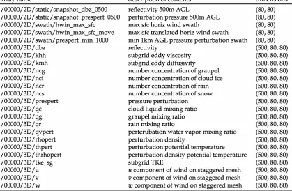
300 node that is participating in writing data opens its unique HDFS file, which creates an empty HDFS 301 file on disk and in memory (data to the disk file is only written when the file in memory is closed). 302 When it is time to write data, a single core on each participating node collects data (using MPI_Gather) 303 from the remaining cores for each requested variable to be written and assembles it into a continuous 304 block of model data that is then written to memory. Following the first write, subsequent writes build 305 the HDFS files in memory with each new time resulting in a new base-level group (see Table 2). When 30• the number of times buffered to memory reaches a user-selectable value (in this case, 50), all groups
301 and files are closed, which flushes the files to disk. Then, new uniquely named directories are created
308 to house new files, and the process repeats until the model finishes.
309 For simulations in which data is saved at a very small time interval, the best performance is 310 achieved when a large number of model times are buffered to memory. This is accomplished by
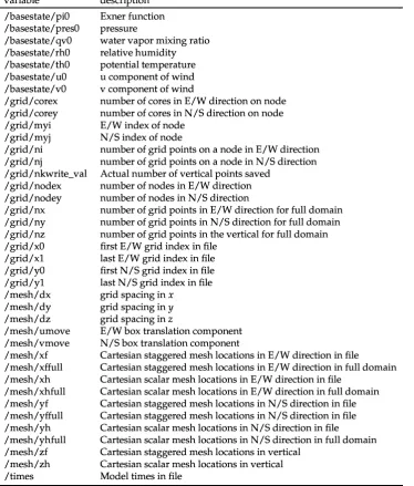
m creating a new base level group that is a zero-padded integer corresponding to the time index (starting m with 0) being written. Groups are a useful way to organize data in HDFS files, and they are also m used to organize metadata, mesh, and the base state sounding data. Table 1 contains a listing of the
variable /basestate/piO /basestate / presO /basestate/ qvO /basestate/rhO /basestate/thO /basestate/uO /basestate/vO / grid/ corex / grid/ corey /grid/myi /grid/myj /grid/ni /grid/nj
/ grid/ nkwrite_ val / grid/ nodex /grid/ nodey /grid/nx /grid/ny /grid/nz /grid/xO /grid/xl /grid/yo /grid/yl /mesh/dx /mesh/dy /mesh/dz /mesh/umove /mesh/vmove /mesh/xf /mesh/xffull /mesh/xh /mesh/xhfull /mesh/yf /mesh/yffull /mesh/yh /mesh/yhfull /mesh/zf /mesh/zh /times description Exner function pressure
water vapor mixing ratio relative humidity potential temperature u component of wind v component of wind
number of cores in E/W direction on node number of cores in N /S direction on node E/W index of node
N /S index of node
number of grid points on a node in E/W direction number of grid points on a node in N /S direction Actual number of vertical points saved
number of nodes in E/W direction number of nodes in N /S direction
number of grid points in E/W direction for full domain number of grid points in N /S direction for full domain number of grid points in the vertical for full domain first E/W grid index in file
last E/W grid index in file first N/S grid index in file last N /S grid index in file grid spacing in x
grid spacing in y grid spacing in z
E/W box translation component N /S box translation component
Cartesian staggered mesh locations in E/W direction in file
Cartesian staggered mesh locations in E/W direction in full domain Cartesian scalar mesh locations in E/W direction in file
Cartesian scalar mesh locations in E/W direction in full domain Cartesian staggered mesh locations in N /S direction in file Cartesian staggered mesh locations in N/S direction in file Cartesian scalar mesh locations in N /S direction in file
Cartesian scalar mesh locations in N/S direction in full domain Cartesian staggered mesh locations in vertical
Cartesian scalar mesh locations in vertical Model times in file
316 the floating point data that contains the model state, the author chose to write identical redundant
317 metadata to all HDFS files. Such redundant metadata includes the number of nodes and cores per
318 node used in the simulation, Cartesian mesh coordinates and dimensions of the full model domain, the
310 model base state (from the CMl input_sounding file) mapped to the vertical mesh, etc. Routines for
320 interrogating and reading in LOFS data exploit this redundancy as "any file will do" to retrieve enough
321 metadata to describe and assemble any subdomain of the simulation. The /times dataset contains
322 the floating point model time that corresponds to each saved time level within the file. Metadata that
m varies between files includes the grid indices and Cartesian location with respect to the full model
324 domain that are contained in the file.
array name description of contents dimensions
/00000/2D/static/snapshot_dbz_0500 reflectivity 500m AGL (80, 80) /00000/2D/static/snapshot_prespert_0500 perturbation pressure 500m AGL (80, 80)
/00000/2D/swath/hwin_max_sfc max sfc horiz wind swath (80, 80)
/00000/2D/swath/hwin_max_sfc_move max sfc translated horiz wind swath (80, 80) /00000/2D/swath/prespert_rnin_1000 min 1km AGL pressure perturbation swath (80, 80)
/00000/3D/dbz reflectivity (500, 80, 80)
/00000/3D/khh subgrid eddy viscosity (500, 80, 80)
/00000/3D/kmh subgrid eddy diffusivity (500, 80, 80)
/00000/3D/ncg number concentration of graupel (500, 80, 80)
/00000/3D/nci number concentration of cloud ice (500, 80, 80)
/00000/3D/ncr number concentration of rain (500, 80, 80)
/00000/3D/ncs number concentration of snow (500, 80, 80)
/00000/3D/prespert pressure perturbation (500, 80, 80)
/00000/3D/qc cloud liquid mixing ratio (500, 80, 80)
/00000/3D/qg graupel mixing ratio (500, 80, 80)
/00000/3D/qr rain mixing ratio (500, 80, 80)
/00000/3D/qvpert perterubation water vapor mixing ratio (500, 80, 80)
/00000/3D/rhopert perturbation density (500, 80, 80)
/00000/3D/thpert perturbation potential temperature (500, 80, 80)
/00000/3D/thrhopert perturbation density potential temperature (500, 80, 80)
/00000/3D/tke_sg subgrid TKE (500, 80, 80)
/00000/3D/u u component of wind on staggered mesh (500, 80, 80)
/00000/3D/v v component of wind on staggered mesh (500, 80, 80)
/00000/3D/w w component of wind on staggered mesh (500, 80, 80)
Table 2. A listing and description of 2D and 3D arrays stored within a single HDF5 file for the 10-m run for the first of fifty stored times. All 3D arrays are shown, but only 5 of 48 2D arrays are shown for brevity. The top level group is a zero-padded index corresponding to the time level stored in the file, starting at 0 (and ending at 49 for this run). The 2D subgroup contains two subgroups of its own: static contains 2D horizontal snapshots of model prognostics and diagnostics while swath contains horizontal slices of statistical properties. The levels above ground of each 2D slice are chosen by the user. The 3D subgroup contains all of the chosen three-dimensional floating point model prognostics and diagnostics. Each 2D and 3D floating point array is a continuous chunk of the full physical model domain that can be viewed independently, but is typically used as a building block for the assembling of larger subdomains for conversion to file formats such as NetCDF, or read in directly to an array for analysis or visualization.
32s Table 2 contains a listing of 2D and 3D floating point data found in each HDFS file. These include
326 two-dimensional horizontal patches of user-selected static variables at various model heights, CMl
321 "swath" variables that provide a statistical look at both mesh relative and ground relative quantities
328 over time, and 3D data describing the model's state. The top level group is a zero-padded index
m describing what time level (starting at 0, and ending at 49 in this example) is being saved in the file,
330 with the 2D and 3D subgroups indicating the rank of the arrays that follow. Actual array dimensions
331 are also found in the listing; for 2D arrays, they are in ( ny, nx) order and ( nz, ny, nx) order for 3D
symbolic notation history
String 3D TTTTT ttttttt nnnnnnn NNNNNNN
Example history E1Reno10m-a 3D
05000 2000000 0009000 0009151
description
Prefix always used for history data User supplied descriptive string
Indicates the directory contains three-dimensional data zero padded integer time in seconds
fractional part of time in seconds
node directory containing files on nodes 9000-9999 node number of file
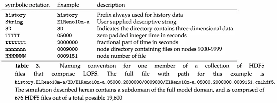
Table 3. files that
Naming convention comprise LOFS. The
for one full file
member of with path
a collection of HOPS for this example is history.E1Reno10m-a/3D/E1Reno10m-a.05000.2000000/0009000/E1Reno10m-a.05000.2000000_0009151.cm1hdf5. The simulation described herein contains a subdomain of the full model domain, and is comprised of 676 HDFS files out of a total possible 19,600
333 3.5. Directory layout and file naming convention
334 A set of Fortran95 subroutines constructs the total path and filename for each HDF5 file based 335 upon strict rules, with variations in the file and directories that are a function of the node number and 336 time of the first saved time within the HDF5 file. The naming convention is demonstrated by first 337 looking at the full path to a single file, corresponding to a file written by node number 9151 starting at
338 time=5000.2000000 seconds:
330 history.E1Reno10m-a/3D/E1Reno10m-a.05000.2000000/0009000/E1Reno10m-a.05000.2000000_0009151.cm1hdf5 340 The naming convention is as follows:
341 history.String/3D/String.TTTTT.tttttttt/nnnnnnn/String.TTTTT.ttttttt_NNNNNN.cm1hdf5
342 Table 3 describes the components of the entire path and file name. The hierarchy within LOFS data is 343 based upon model time, with new directories whose name contain the floating point model time being 344 created for each time data is flushed to disk. In order to avoid performance issues related to having
345 too many files in a single directory, data is spread in 1000 file chunks in subdirectories whose names 346 are simply a sequence of zero-padded factors of 1000.
347 In the simulation described below, a maximum of 1000 HDF5 files will be found in any node
348 subdirectory. Spreading the many files that make up a simulation amongst many directories has been 340 found to produce much better performance than placing them all in one directory. In the example 350 above, node directory 0009000 would contain, for a simulation in which the full domain was saved, a 351 thousand files with node numbers 9000 through 9999.
352 It should be emphasized that on the read side, metadata is extracted from the file and directory 353 names themselves (in addition to retrieving metadata from files) in order to reconstruct the full domain 354 space such that the proper files can be accessed when users request data. Further, because of the 355 high temporal frequency of data saved in this simulation (in this case, every 0.2 s), the time string in
356 seconds embedded within the HDF5 files is actually a floating point representation of the time that is 357 then converted to floating point data in the read-side code. Because each HDF5 file contains 50 time 358 levels in this simulation, the HDF5 time embedded within the file name descriptor refers to the first of 3so 50 times contained within the file, with all saved times comprising the /times dataset (a 1D double
300 precision array) stored in each file.
361 By enforcing strict file and directory naming conventions, read-side applications programmed 352 with knowledge of these conventions (or using the existing LOFS read-side routines) can traverse
argument --time=5400.0 --offset --x0=800 --y0=750 --x1=1300 --y1=1250 --z1=300 --histpath=3D --base=torscale-10m --swaths
--nthreads=4
thrhopert prespert ...
description Select t
=
5400Indices are with respect to what was saved, not the full domain origin (0,0) west boundary index
south boundary index east boundary index north boundary index top boundary index
Top level 3D LOPS directory base name given to netcdf files Retrieve and save all swaths
Number of OpenMP threads to use for calculations The variables requested
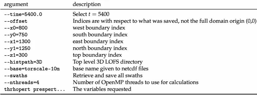
Table 4. Description of command line arguments to lof2nc such as those used to create NetCDF files that are shown in all storm imagery in this paper.
366 3.6. Reading data from LOFS
361 For reading LOFS data, routines written in C have been created that provide a way to access 368 any saved variable at any time spanning any arbitrary subdomain found within the LOFS data. To
m demonstrate, an example of the lofs2nc utility is described below, creating a NetCDF file containing
310 all of the 2D found within a subset the LOFS data as well as selected 3D data.
m Consider a situation where a user wishes to make a NetCDF file that spans the region immediately
312 surrounding the tornado in the simulation for visualization. This is achieved with lofs2ne, a front end 373 to a series of underlying routines that traverse the LOFS structure to extract metadata from directory 374 names and file names, reads redundant metadata from one of the HDF5 files, and then loops across
375 files, incrementally filling a buffer with user-requested data. An example command follows:
376 lofs2ne --time=5400.0 --offset --x0=800 --y0=750 --x1=1300 --y1=1250 --z1=300 \
311 --histpath=3D --base=torseale-10m --swaths --nthreads=4 \
318 thrhopert prespert uinterp vinterp winterp xvort yvort zvort qe qr qg neg ner dbz
m Table 4 breaks down the different options to the above lofs2nc command. The user has requested
380 a 501 (in x) by 501 (in y) by 301 (in z) volume of data whose indices are relative to the origin of the 381 file corresponding to the lowest saved node number. The user has requested a list of variables, some 382 of which are read directly from the LOFS data (thrhopert, prespert, qe, qr, qg, neg, ner, dbz) and
383 some which require calculation based upon other saved data (uinterp, vinterp, winterp, xvort, 384 yvort, zvort). Due to the large amount of data produced by simulations run at this scale, the author 385 has chosen a save strategy that focuses on saving the minimum number of 3D arrays needed to 386 calculate any possible other diagnostic/ derived fields and calculating those fields on the fly (with
381 calculations parallelized using OpenMP on multicore machines). For instance, the LOFS data saved 388 for this simulation saved the native u, v, and w CMl variables that lie on the staggered Arakawa C 3so grid [36) such that the velocity components interpolated to the scalar mesh, as well as the vorticity
390 components interpolated to the scalar mesh, are calculated within the lofs2nc code. This specific 391 strategy ensures that the highest amount of accuracy is preserved for all calculations involving velocity 302 variables in methods consistent with those done within the CMl model.
393 The process by which the LOFS read-side code retrieves metadata involves an entire traversal of 394 the saved directory structure as well as reading metadata from at least one of the HDF5 files in each
m time directory. These combined operations can take dozens of seconds to complete when hundreds to
396 thousands of time levels are saved, but because the results of these operations always return identical 397 information, the caching of this information is done the first time the command is run, and cache files
399 requiring the formatted reading of several small text files), leaving the code to spend its time to read and write and, if requested, calculate derived variables.
400
401 Pseudocode for lofs2nc is found below. Note that the first four routines will first check for cache
402 files and read from these if they exist; otherwise, the LOFS directory structure is traversed and, using
403 routines of the dirent C library, file names within directories are read, sorted, and a single HDF5 file
404 is selected for internal metadata acquisition. Cache files are written if they do not exist, such that this
405 process only occurs once, and does not need to be done again until the LOFS file structure is modified
406 (for example, by adding more time levels as a simulation progresses through time).
407
408 get_num_time_dirs !get number of top level directories in 3D directory �• get_sorted_time_dirs !get the directory names and sort using quicksort 410 get_sorted_node_dirs ! get a sorted list of the zero-padded node directories u1 get_all_available_times !get a list of every time level saved in all the data 412 get_available_3D_variable_names ! get a list of all 3D variable names
03 get_LOFS_metadata_from_a_HDFS_file !get mesh, grid, and basestate information 414 initialize_netcdf ! Set dimensions, attributes, and define requested variables 41s if get swaths: get_all_swaths; write_all_swaths ! All 2D fields read and written ue get_data_to_buffer !Buffer variables for diagnostic calculations, if requested 417 for each requested variable:
418 419 420
if exists_in_LOFS and not_already_buffered: read variable into buffer if is_diagnostic: calculate diagnostic into buffer
write_requested_quantity_to_netcdf_file
421 Following metadata acquisition, the list of requested variables is checked against what is available, and,
422 if diagnostic quantities (such as vorticity components) are requested, temporary arrays are allocated
423 and a flag is set to indicate which LOFS variable is needed for the diagnostic quantity for buffering
424 to memory. As an example, if the vertical component of vorticity(') was requested (called zvort in
425 CMl/LOFS), u and v would be buffered to their own arrays such that zvort could be calculated. If u
426 and v were also requested for writing to NetCDF files, these buffered values would be written without
427 re-reading LOFS data. Hence, the code only allocates memory for what is needed and re-uses buffered
428 variables when needed. The main loop over variable names contains code for calculating diagnostic
420 quantities, and new quantities can be added at the end user's leisure.
430 All LOFS HOF operations are serial, and this is also true with lofs2nc. However, because
431 modern supercomputers use parallel file systems, excellent performance is found executing serial
432 1/0 operations in parallel by writing scripts that execute many instances of lofs2nc concurrently.
433 This workflow is nearly always used since a main motivation for LOFS is doing analysis at very high
434 temporal resolution. Running several instances of any code is easily achievable using shell scripting
435 where jobs are forked into the background. A tremendous amount of data can be read and written
436 quickly in this manner, exploiting the inherent parallelization of the operating system running on a
437 multicore machine and reading (writing) from (to) a parallel file system such as Lustre or GPFS.
438 3.7. The use of ZFP compression
439 The primary motivation of the development of LOFS was to enable the saving of very high
440 resolution data at extremely high temporal resolution. This combination will, without care, result in
441 unacceptably poor model 1/0 performance due to insufficient 1/0 bandwidth, as well producing as
442 an overwhelmingly large amount of data. LOFS offers, through the use of input parameters in the
443 namelist. input file that CMl reads upon execution, the ability to save only a subset of the model
444 domain, which is practical when one is interested in studying the region of the storm directly involved
44s in tornado processes near the ground. In the simulation described below, a volume spanning 2,080
446 by 2,080 by 500 grid points (corresponding to 20.8 km by 20.8 km by 5 km in x,
y
and z respectively)447 was saved in LOFS files from t = 5000.2 s through t = 7490 s, spanning 0.86% of the volume of the
448 full model domain (see Fig. 3 to see the horizontal extent of saved data). However, this reduction still
450 over the life cycle of the tornado. In order to reduce the amount of data saved to disk to a reasonable 451 value, ZFP [25] floating point compression was used.
452 ZFP uses a lossy algorithm that results in three-dimensional floating-point data that contains
453 less than the original 32 bits of precision after being uncompressed. However, the resulting data
454 exhibits compression performance that (usually) far exceeds that of lossless compression algorithms.
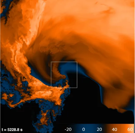
455 Further, an attractive aspect of ZFP is that it offers a dynamic compression option whereby the absolute 456 maximum amount of accuracy required for each value in each 3D array may be specified, and that 457 this accuracy parameter is specified in the same units as the saved data. For instance, in the supercell 458 simulation, simulated reflectivity (shown for example in Fig. 3) is saved in order to create plots that 450 can be compared to real radar observations of supercells. This variable is used for plotting purposes 460 only, and will never be differentiated or used in post hoc analysis in equations where high amounts 461 of accuracy are needed. A value of 1 dBZ was chosen as an accuracy parameter for the dbz variable, 462 which means every value in the uncompressed 3D dbz arrays will exceed 1 dBZ of accuracy. ZFP's 463 algorithm is conservative, and in reality, the accuracy of the data will typically far exceed this specified 464 value throughout the 3D arrays.
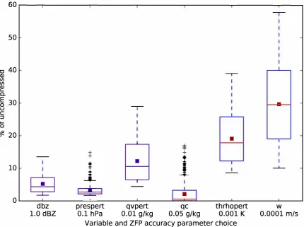
465 Figure 2 provides a box and whiskers plot of compression performance for several 3D variables 466 at a snapshot in time when the tornado is mature and exhibiting a multiple vortex structure. These
467 statistics were chosen from all 676 files spanning the saved subdomain. Data within this subdomain
468 contains regions of both weak and sharp gradients, and the widely varying compression performance 460 in this example reflects this. For the aforementioned dbz variable, which was saved with 1.0 dBZ 410 accuracy, the space taken by the 3D array was 5.2% of its uncompressed size, providing an average 471 compression ratio for this variable of approximately 19:1. Had a larger accuracy parameter been 412 chosen, compression performance would have increased accordingly.
473 Because future post hoc analysis will involve Lagrangian trajectory analysis and the effects of lossy 474 compression on trajectory performance have yet to be determined by the author, a very small value 41s (0.1 mm s-1) was chosen for each of the three components of velocity, each of which exhibited very 476 similar compression performance. This resulted in an average reduction to 30% of uncompressed, 411 or roughly a 3:1 average compression ratio, with values ranging from 10% to 58% of uncompressed 478 across all saved files. This wide variation in compression performance across files is indicative of
410 the dynamic nature of ZFP compression, where regions of large gradients result in less compression
480 than regions of weaker gradients. The prespert variable (perturbation pressure in hPa) shows several 481 outlier compression reductions that correspond to regions of abnormally large gradients that are found 482 along the length of the tornado (which is tilted, spanning several files) and other weaker vortices. 483 The cloud mixing ratio variable qc exhibits compression performance in some files where nearly no 484 data is saved, corresponding to cloud free areas of the simulation, but also many outliers where large 485 gradients are found within the cloud including along the periphery of the condensation funnel of the
480 tornado.
60.---.---..---,---.---r---.---,
50
"O 40
QJ
I
---r-l/l
l/l I
QJ
§
30-1
-
-"#. 20
10
8
0
dbz 1.0 dBZ
g
t
j_
�
prespert qvpert
0.1 hPa 0.01 g/kg
+
1
•
qc 0.05 g/kg
I
•
I
thrhopert 0.001 K Variable and ZFP accuracy parameter choice
I I
----'--w 0.0001 m/s
Figure 2. A Tukey [37] box and whiskers plot of compression performance statistics (in terms of percentage of uncompressed size) of six of the saved variables within the 676 files spanning the full saved subdomain, which is roughly centered on the tornado. The green line represents the median value, the red square the mean value, while the box contains the interquartile range (IQR) with the bottom and top whiskers within 1.5 IQR of the lower and upper quartile, respectively. Outliers are plotted with the '+' symbol. The accuracy parameter chosen at runtime is noted below each of the 3D variables names. Larger (smaller) values of the accuracy parameter would have resulted in smaller (larger) file sizes. Variables displayed are simulated reflectivity (dbz, in dBZ), perturbation pressure (prespert, in hPa), perturbation water vapor mixing ratio (qvpert, in g/kg), liquid cloud water mixing ratio (qc, in g/kg), perturbation density potential temperature (thrhopert, in K) and vertical wind speed (w, in m/s). The mean compression performance for the shown variables is 11.9% of uncompressed, or a compression ratio of 8.4:1
494 4. The 10 m resolution tornadic supercell simulation
49s The simulation was run on an isotropic mesh with a grid spacing of 10 m, in a box spanning
496 112km by 112km by 20km (using 11, 200 x 11, 200 x 2000, or 250,880,000,000, grid points). A model
497 time step of 0.04 s was used in order to maintain stability, and a short time step of 0.01 s was used for
498 the acoustic time step. The chosen time step is smaller than what was necessary for computational
499 stability due to aliasing; however, a larger time step resulted in sporadic failure of CMl's saturation
soo adjustment scheme, which is iterative, to converge, causing the model to abort. The remaining model
501 parameters were identical to those of [17] with the exception that the TKE closure option of Deardorff
503 4.1. Execution of the simulation on Blue Waters
504 The supercell simulation was executed on the Blue Waters supercomputer in 22 segments between
606 April 19 and August 2, 2019. Each segment of the simulation beyond the first was run from checkpoint
606 files that were saved in HDF5 format with all 3D state variables compressed with lossless gzip
507 compression. The simulation took approximately ten million node hours (320 million core hours) in
508 total to run to a model time of 7490 s, a few minutes after the cyclonic tornado fully dissipated. This
m corresponds to just over 21 days of execution using 87% of all available XE nodes on Blue Waters.
510 Each segment of the simulation ran on 19,600 nodes (672,200 cores) when executing, with a
m maximum requested run time of 48 hours per segment, the largest allowed on the machine. However,
512 when running over such a large portion of the machine, node failures were common, occurring on
513 average four times per 48 hour block. These node failures were out of the author's control and not due
514 to model instability or any other failure of the CMl model. When a node failure occurred, a message
m such as the following would appear in the CMl standard output file:
510 [NID 19080] Apid 78797135 killed . Received node event ec_node_failed for nid 19075
617 Consultation with Blue Waters support staff indicated that these node failures occurred on the Opteron
518 processors with a return value of C0MPUTE_UNIT_DATA which indicates an uncorrectable error occurring
519 on one of the node's CPUs. Recognizing the regularity of these types of unavoidable errors, the author
520 chose to save checkpoint files every 10 model seconds, and, via a loop within the PBS script file, restart
521 the model from the most recent checkpoint file automatically such that the entire requested reservation
522 time could be used. This required the allocation of a handful of extra nodes for each job submission as
523 a reserve such that there were enough healthy nodes available for each execution, as the failed nodes
624 would be removed from the pool. With these issues in mind, it is estimated that about a quarter of the
525 utilized node hours on the machine were "wasted" due to these failures.
52e Because it was not known whether the simulation would produce a long track EF5 tornado
527 similar to [17], full domain data was saved only every 10 s until the beginning of tornado maintenance
628 was observed. Then, using one of the saved checkpoint files, the model was restarted from a time
52• approximately 10 minutes prior to tornadogenesis and subsequent data was saved over a smaller
530 subdomain with a save interval of 0.2 s until tornado decay occurred. The 10 s full-domain data, saved
531 between
t
= 1800.0 s andt
= 4990 s comprised 83 TB of LOFS data, while the subdomain data saved532 every 0.2 s from
t
= 5000.2 s andt
= 7490 s weighed in at 187 TB.633 4.2. A first look at tornadogenesis
534 Here a description of the process of tornadogenesis is provided, focusing primarily on the growth
636 of near-ground vorticity. The model times of the figures following in this section were chosen after
636 creating a video animation of the 0.2 s data and stepping forwards and backwards through the video
637 until key moments in the simulation were identified. It should be emphasized that only a topical
538 analysis of tornadogenesis is provided in this section, and that a more exhaustive quantitative analysis
639 is beyond the scope of this paper. The supplemental video file SupVl of the vorticity magnitude
540 field and surface maximum vertical vorticity swaths from
t
= 5000 s throught
= 5390 s is found at541 http:// orf.media/ Atmosphere2019. This video sequence begins approximately three minutes prior
542 to tornadogenesis and continues through about three minutes of tornado maintenance, with frames
543 displayed every 0.2 s at 30 frames per second.
544 Figures 4-6 provide an overview of cyclonic vortex paths, superimposed upon density potential
646 temperature perturbation (0�), to provide a context for the more information-dense three-dimensional
540 images in subsequent figures (these images originated from the output of the ncview [41] utility,
647 read from NetCDF files created with lofs2nc). The bulk of surface vortices identified by swaths of
548 maximum vertical vorticity (s') shown in Figs. 4-9 originate on the cold (west) side of what [42] call
540 the Left Flank Convergence Boundary (LFCB) (see their Fig. 8). This boundary is clearly visible in
5so both the surface horizontal wind and
e�
fields, with its location along the sharp 0� gradient noted inFigure 4. Density potential temperature perturbation (0�) in K att
=
5000.2s. Horizontal domain covers 4km x 4km. Black swaths are the ground-relative paths of cyclonic vortices at the model's lowest vertical level (motion is generally southward to eastward). The sharp 0� boundary representing the Left Front Convergence Boundary (LFCB) is noted. The color map indicates values of 0� in K.0
3
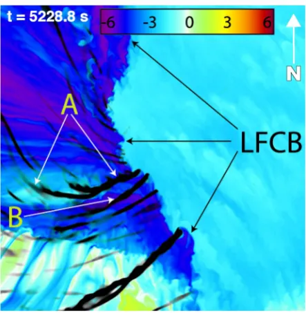
Figure 6. As in Fig. 5 but at t = 5228.8 s, corresponding to the same time in Fig. 3.
m range from southward to eastward, with many paths abruptly turning from southward to eastward
553 (see Fig. 4) along their respective paths. Three minutes later, at
t =
5183.0 s, the incipient vortex that554 "becomes" the tornado (tagged to as vortex A in subsequent figures) has turned from southeastward
555 to eastward and has begun to produce a 20 m swath of instantaneous ground-relative winds just
556 exceeding 39 m s-1, the EFl threshold. The direction of vortex paths to the south of vortex A seen
557 in Fig. 5 exhibit a slight to moderate northward component, indicating a convergence of vortices
558 occurring in its direct vicinity. At this time, vortex A is located along an inflection point in the LFCB,
559 which is oriented directly north/ south to its north, and towards the SSE to its south. The reorientation
560 of the LFCB is seen to persist in Fig. 6, 46 s later, with the LFCB showing an eastward bulge consistent
561 with an increase in eastward momentum to the south of vortex A, which is now exhibiting a 40 m
562 swath of EF2 strength winds (averaging 55 m s-1 ). A second vortex, vortex B noted in Fig. 6, follows a
563 convergent path with vortex A and is discussed below.
564 Figures 7-9 provide six snapshots in time, the first two of which overlap with Figs. 5 and 6. These
565 images were created with the NCAR's VAPOR3 software [40], which can read NetCDF files containing
566 2D and 3D floating point data natively. The left panel of these images contains three-dimensional
567 volume rendered vorticity magnitude with a visible threshold value of approximately 1.25 s-1, along
s68 with surface maximum i; swaths that can be matched with those in Figs 5 and 6. SupVl corresponds to
569 the left panels of these figures, while the right panels present a different viewing angle, and include,
510 in addition to surface maximum i; swaths, the liquid cloud water mixing ratio (qc) field to show the
511 behavior of the condensation funnels associated with strong rotation. In Fig. 7a, vortex A can be seen
512 extending upwards from the ground but is not associated with a visible condensation funnel at this
m time. In Fig. 7b, 45 s later, vortex A has strengthened at the surface and extended upwards to a height
574 of nearly 3 km. A second vortex, vortex B, is also visible, having formed in a similar "bottom-up"
575 manner as vortex A, and is in the process of being assimilated into the circulation of vortex A. Both
576 vortices are associated with visible condensation funnels also seen in Fig. 7a. Figure 8a shows the
511 same fields 44 s later, where vortex A is exhibiting a 50 m wide swath of EF3 strength surface winds
578 (averaging 70 m s-1) with another vortex, vortex C, having just swept behind the path of vortex A and
m extending upwards to a height of approximately 1 km. Vortex A is now "the tornado" as is evidenced
580 by its co-location with a columnar condensation funnel that extends from the parent supercell cloud
581 base to the ground. Over the next 12 s, vortex C has grown upward to a height of exceeding 2 km and
683 clearly in SupVl where the two vortices wrap around one another in a "bottom-up" manner. While 584 mergers of helical vortices in three dimensions have been observed and modeled [43,44], the author 585 is unaware that this phenomenon has ever been seen in an observed supercell or in simulations of 686 a supercell. By
t
= 5307 s, when the wrapping process has extended to a height of approximately 687 2.5 km, the tornado is exhibiting EF5 surface winds exceeding 105 m s-1 (see Fig. 9a). A minute later, 688 the tornado's diameter has widened, as is evident from the size of the visible condensation funnel and 589 maximum , swath field, and has also assumed a more vertically erect position, and is moving in a 590 linear fashion towards the northeast. Maximum instantaneous surface winds exceeding 140 m s-1 are 591 found at this time, shortly before the tornado obtains a multiple vortex structure.592 5. Discussion and Future Work
593 In this paper, LOFS, a simple file system designed for saving large amounts of massively parallel
694 cloud model data efficiently, was described, along with a use example of a the lofs2nc utility for
595 converting LOFS data to the widely-read NetCDF format. NetCDF files created from lofs2nc by the 596 author were then read and displayed with ncview [41] (Figs.�) and VAPOR3 [40] where 3D images 697 were created (Figs. 7-9) and saved to disk to be statically viewed as well as animated (SupVl). The 698 author's experience with running the simulation on 19,600 Blue Waters nodes (672,200 cores), spanning 699 87% of the supercomputer's XE nodes, was described, which included a process for recovering 600 from node failures automatically by restarting the model from the most recent checkpoint files. The 501 performance of dynamic ZFP lossy floating point compression was described for six 3D fields saved 602 by CMl, with each variable having maximum accuracy specified at runtime. The use of ZFP and the 603 choice of saving a small subdomain, focused on the low level mesocyclone, allowed data to be saved 604 every 0.2 s, and this 1/0 approach took up a reasonable 37% of the model's execution time. A total 606 of 270 TB of data was saved, with 83 TB of full domain data saved in 10 s intervals from
t
= 1800 s 606 throught
= 4990 s, and the remaining 187 TB of data saved fromt
= 5000.2 s andt
= 7490 s over a 607 20.8 km by 20.8 km by 5 km subdomain every 0.2 s.608 Visualizations of the vorticity and cloud field reveal a process of tornadogenesis characterized 609 by the convergence, merging, and upward growth of several near-ground vortices, one of which 610 wraps around the nascent tornado in a bottom-up fashion. The tornado forms along the Left Front
m Convergence Boundary [42] which is prominently displayed as a sharp buoyancy gradient in the cold
512 pool. A few minutes prior to tornadogenesis, vortices on the cold side of this boundary take a sharp
m turn towards their left (moving southward to eastward) and then begin to travel towards the north
614 east. Genesis occurs shortly thereafter, with the tornado forming along an inflection point in the LFCB, 616 which has surged forward to the south of the developing tornado. While only a topical discussion of 616 tornadogenesis, focusing on vorticity, has been presented, the value of using 3D volume rendering 617 software such as VAPOR3 [40] has been clearly demonstrated, with animations of vorticity at full 0.2 s 618 frame spacing telling a compelling story. Only one aspect of the tornadogenesis process has been 519 presented here, and only over a short span of time; the tornado lasts 42 minutes and transitions to a 520 wide, multiple vortex tornado that eventually becomes occluded before dissipating.
521 Much future work needs to be completed in order to quantify the complex morphology of the 622 simulation. Such work will include:
623 624 625 626 627
628
629
630 631
• The use of temporal averaging to "smooth out" the details of the simulation in order to focus on underlying, steady forcing prior to and during tornadogenesis
• Examining the momentum and pressure characteristics of the updraft prior to and during tornado formation.
• Conducting Lagrangian parcel analysis to explore the forces acting on parcels in the vicinity of the tornado