Foldover search designs with error and augmenting runs

(1)

VICTORIA

~

UNIVERSITY

DEPARTMENT

OF

COMPUTER AND MATHEMATICAL

SCIENCES

FOLDOVER SEARCH DESIGNS

WITH ERROR AND AUGMENTING

RUNS

Neil T. Diamond

(19 E.Q.R.M. 9)

TECHNICAL REPORT

VICTORIA UNIVERSITY OF TECHNOLOGY

BALLARAT ROAD (P 0 BOX 64) FOOTSCRA Y

VICTORIA, AUSTRALIA 3011

TELEPHONE (03) 688-4249/4492

FACSIMILE (03) 687-7632

Campuses at

Footscray, Melton,

..

... n %

z

0

,..

(2)

FOLDOVER SEARCH DESIGNS WITH ERROR

AND AUGMENTING RUNS

Neil T. Diamond*

Victoria University of Technology

Summary

The performance of a class of two-level nonorthogonal resolution IV designs with n factors when experimental error is present is

investigated and the design of augmenting trials discussed and illustrated with an example. If a block effect needs to be taken into account then only two augmenting trials are required with up to five factors and three augmenting trials with up to nine factors.

[( ey Words: Fractional factorial designs; nonorthogonal designs; reso-lution IV designs.

1. Introduction

The most common resolution IV designs used in practice and discussed in the literature are orthogonal. For these designs the main effects are estimable and unbiased by two-factor interactions while the two-factor interactions are usually aliased with each other.

(3)

In a previous paper, (Diamond, 1991), it was shown that the class of modified one-factor-at-a-time foldover designs, consisting of all one-letter runs and all ( n - 1 )-letter runs for n two-level factors, can be considered as search designs (Srivastava, 1975). When there is no error a strongly resolvable search design of resolving power k provides, in this context, esti-mates of the mean and all main effects and allows the search and estimation of the real two-factor interactions, assuming the maximum number of real two-factor interactions is k; while a weakly resolvable search design only allows this for some values of the two-factor interactions. The modified one-factor-at-a-time fol dover designs are strongly resolvable when k = 1; weakly resolvable when k

=

2 except when the number of factors is 6; and may not be even weakly resolvable when k ~ 3.

In this paper the above results are extended to cover the case when experimental error is present and also to illustrate the design of augmenting trials which may be needed if the real two-factor interactions take on certain values.

2. An

Exa111ple

Box, Hunter and Hunter (1978, p.377) illustrated the use of a 25- 1 fractional factorial design by re-analysing a 25 design but only using the results of the runs in the 25- 1 design. The five factors were 1, feed rate; 2, catalyst; 3, agitation rate; 4, temperature; and 5, concentration; while the response was the percentage of a raw material reacted in a reactor. For convenience in this paper the five factors have been re-labelled B, D, C, A and E respectively. Table 1 gives the results of the ten runs in the 25 experiment correspond-ing to the modified one-factor-at-a-time foldover design. Table 2 gives the mean square errors for the regression of the five main effects on the response and also for the best five models when fitting one and two interactions in addition to the main effects where, for example, {AD, AE} corresponds to the model where the main effects A to E are fitted as well as the two-factor interactions AD and AE.

(4)

Run Factor Response

A B

c

D E (%reacted)

1

₊

- - - _- ₆₉

2 -

₊

_ I _-

_-

₅₃

3 - -

₊

- - 53

4 - I

-

-+

-

63

5 - -

-

₊

56

6 -

_{+ + + +}

₆₅

7

₊

'

-+ -+ -+

81

8

_{+ +}

-

_{+ +}

77

g

_{+ + +}

_-

₊

₄₂

10

_{+ + + +}

- I ₉₈

'

•

Table 1: Results of the 10 runs in a 25 experiment corresponding to the modified one-factor-at-a-time foldover design.

Number of Interactions MSE

interactions in model

0

{ }

152.90

1 {CD} 96.53

{BE} 115.67

{AE} 115.67

{BD} I

125.19

{AD} ' 125.19 '

2 {CD,CE} 1.79 i

{AD,AE} 5.50

{BD,BE} 5.50

'I

{AE, BC} 52.00

{AC,AE} 52.00

(5)

two two-factor interactions. If we assume that there are at most two non-zero two-factor interactions then it appears likely that one of these three models is the correct one. Analysis of the full 25_,_{with the regression parameterization}

used in this p~er, shows that the true model is in fact {AD,AE} with

AD

=

6.625 and AE

=

-5.5.

The fact that these three models are the best is in line with the findings in the previous paper. There it was shown that when the true model consists of two interactions with one letter in common and the interaction effects equal in magnitude but opposite in sign, then searching for the true model in the error-free case is not possible since the component of the observation vector orthogonal to the mean and main effects lies in the subspaces corresponding to a number of different models. The example illustrates that, even when the interaction effects are only approximately equal in magnitude and opposite in sign, it will be difficult to distinguish between the models corresponding to the intersecting subspaces on the basis of the data if error is present. As shown in a later section it is possible to design augmenting trials to resolve these ambiguous results.

3. Perfor1nance of the Designs with Error

In the example a number of models had similar mean square errors. In this section an analysis of the expected value of the mean square error when fitting a false model will be undertaken and applied to the modified one-factor-at-a-time foldover design.

Consider the case where we are fitting a model M2 when the true model is in fact M 1. In the context considered in this paper M1 and M2 would involve the mean, all main effects and ki(i

=

1, 2)

<

(n - 1) two factor interactions respectively where the two factor interactions are different for M1 and 1112.

The true and false models can be rewritten as

Xo/30+X1/31 + t:1

Xo/30

+

X2/32

+

£2

(6)

con-sist of the remaining columns of the design matrices respectively and £_{1 ,...,} N(O, cr2 I) since Af1 is the true model whereas c:2,..., N(Xifli - X2/32, cr2I). Both models can be rewritten as

M1: y.o

M2: y.o

X1.o/31

+

€1 X2.o/32

+

€2

where y.o, X1.0 and X2.o, the matrices of residuals of y,X1 and X 2 regressed on Xo respectively are given by

Y·O (I - Xo(XbXo)-1 Xb)Y

X1.o (I - Xo(XbXo)-1 Xb)X1

X2.o (I - Xo(XbXo)-1 Xb)X2.

When model A12 is fitted then y.0 is projected onto the manifold generated

by the columns of X 2·0. Then the estimated error vector €2 is given by

where the projection operator is

The residual sum of squares is then given by

RSS C:2C:2 ~1 ~

(/3~X~.

₀

+

c:~)(I - P)(X1.o/31

+

€1)

since (I - P) is idempotent. Hence

E(RSS) E(/3~X~.

0 +

£~)(! - P)E(X1.o/31

+

t:1 )

+

trace(cr2(I - P)I)

/3~X~.o(I - X2.o(X~.

0

X2.o)-1X~.

0

)X1.o/31

+

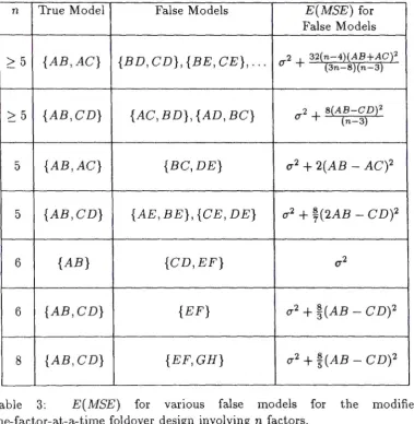
(n - k2 - l)cr2.

In table 3 the expected values of the mean square errors have been

cal-culated using the above formula for the cases where if there were no error

(7)

n True Model False Models E(MSE) for

False Models

I I

~5 {AB,AC}

1

{BD, CD}, {BE, CE}, ... <T2

+

32{n-4l{AB+AC}2 _{3n-8Hn-3}

I

~5 {AB,CD} {AC, BD}, {AD, BC} _<T2

+

B(AB-CD)_{n-3} 2

5 I {AB,AC} {BC, DE} u

2

₊

_{2(AB - AC)}2

5 {AB,CD} {AE, BE}, {CE, DE} u2

+

~(2AB - CD)2

6 {AB} {CD,EF} ()2

6 {AB,CD} {EF} u2 +~(AB - CD)2

I I

8 {AB, CD} {EF,GH} u2 +~(AB - CD)2

(8)

/

M {b24, b34} ,.,,.,,.,,.,,.,,.,

RSS1_l2

~(AB+

AC)(b17 + b13)/2

I

---::....,.1

/

e ,.,

,.,

---/

"

,., "' in direction

Figure 1: Geometric interpretation of the estimation of the two-factor inter-actions BD and CD when the real two-factor interactions are in fact AB

and

AC,

following a modified one-factor-at-a-time foldover design.

Table 3 shows, for example, that if the true model is {AB, AC} and if

AB

=

-AC

then the expected value of the mean square errors will be u2 _for

( n - 2) models. A geometric interpretation of this result and an alternative derivation of E(RSS) is given below and represented in Figure 1.

The manifold orthogonal to the mean and main effects corresponding to the true model {AB, AC} is spanned by the vectors bi2 and bi3 and is denoted by M { b12, bi3}, while the manifold orthogonal to the mean and main effects corresonding to the false model {BD, CD} say is spanned by the vectors

bz.1

and b31 and is denoted by M { b24, b34}, where the bij take the values (4 - 2n)/n in the i th and j th rows and 4/n elsewhere. The

(9)

orthogonal to the mean and main effects, ABb12

+

ACb13, onto bi2 - bi3 is given by (AB - AC)(b12 - b13)/2. The fitted false model component orthogonal to the mean and main effects is given by the vector (AB

-AC)(b12 - bi3)/2 plus the projection of (ABb12

+

ACb13 - (AB AC)(b12 -b13)/2) onto (b24

+

b34) since (b24

+

b34) is obviously orthogonal to (b24 -b4).

Then RSS1_l2

₌

_(AB+_AC)ll(b12

₊

_{bi3)!1(sin 0)/2 where}₀_{is the angle formed}

by (b12

+

b13) and (b24

+

b34). Hence

where

1

RSS

=

4(AB

+

AC)2ll(b12

+

b13)112(1 - cos2 0)

cos()= (b12

+

b13). (b24

+

b34) Cllb12

+

b13ll)(llb24

+

b34II)

and evaluating this, and since the degrees of freedom is ( n - 3), we obtain

MSE

=

32(n - 4)(AB

+

AC)2

(3n - 8)(n - 3)

Since the modified one-factor-at-a-time foldover design is symmetric in all the factors, the results in Table 3 also apply when factor labels are interchanged. For example, taking n

=

5 and interchanging B with D and C with E, we can see that if AD= -AE for the true model {AD, AE} then the falso models {BD,BE} and {CD,CE} will also have E(MSE) = o-2, agreeing with the example covered in the previous section.

The results in table 3 can be used in a number of ways. For example, assume that there exists a good estimate of the standard deviation o-. Then the standardized residual sum of squares ( RSS / o-2) follows a noncentral chi-square distribution with noncentrality parameter

(10)

Number of h

factors , n

5 1.84

6 1.64

7 1.59

8 1.57

9 1.57

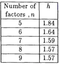
Table 4: Values of h such that

I

AB+ AC I~ her forms a 95% consonance

region for {BD,

CD}

.

For a particular false model M2, a set of values of the true model pa-rameters /31 can be calculated for which the probability of declaring M₂ consonant with M1 is greater than 0.05. We will call such a set a 95% consonance region for M2. The region is calculated by setting

A

so that

where x(v; A) stands for the noncentral chi-square distribution with degrees of freedom v and noncentrality parameter A, v = error degrees of freedom for model M2, and

x

2a(v) stands for the lOOa percentile of the central

x

2 distribution with degrees of freedom v.

With M1 given by {AB, AC} and M2 given by {BD,

CD}

the

conso-nance regions are of the form

I

AB+ AC I~ her. Table 4 gives the values of

h for the modified one-factor-at-a-time foldover design with 5 ~ n ~ 9. If

the values of the two-factor interactions fall outside the consonance region then the probability that the false model can be separated from the true model on the basis of the data will be more than 0.95.

4. The Design of Aug1nenting runs

(11)

the basis of the data is the true model. The designs considered here can also be viewed as examples of "Probing designs" introduced by Srivastava(1989). The emphasis here, however, is quite different in that we deal only with the class of modified-one-factor-at-a-time foldover designs, both the error-free and error cases are covered as is the case when a block term is required.

It suffices to consider only one case in detail corresponding to the n factor design in 2n runs when the two non-zero interactions have one letter in common and opposite effects. We will initially assume the error-free case and without loss of generality relabel the factors so that the i th of the ( n - 2) competing models consists of the interaction between the i th and ( n - 1) th factors and the interaction between the i th and the n th factors, 1

Si S

(n - 2).

For the interaction between the k th and the I th factors (1

S

k

<

I

S

n) the corresponding column in the initial design, orthogonal to the mean, is

bkt and for the augmenting design Bk1. Both bk1 and Bk1 take the value ( 4/ n) in rows where factors k and l take the same levels, and the values (4-2n)/n elsewhere.

In order to separate the i th and j th model (1

S

i

<

j

S

(n - 2)) the column vector

Cij = Bi(n-1) - Bin - Bj(n-1)

+

Bjn

must not be equal to 0, and hence for the augmenting design to be effective all the Cij must not equal 0. Furthermore, if a block effect needs to be allowed for, which is most often the case in industrial experimentation, then the Cij must not be proportional to the unit vector.

Note that

Bl(n-1) - Bln - Bj(n-1)

+

Bjn

[B1(n-l) - Bin - Bi(n-1)

+

Bi(n)]

which equals Cij· Moreover Cij

=

0 if and only if C1j

=

C1i, and Cij

=

xl if and only if C1j

=

Cii

+

xl, that is they differ by a constant amount.

Hence we need only examine the matrix

in order to determine if the augmenting design will separate the (n-2) com-peting models.

(12)

or(-,+,+,-), the value 4 is taken when the sign sequence is(+,-,+,-)

or(-,+,-,+), and the value 0 taken otherwise. The r rows of the matrix

C

can be reordered so that the first r1 S r rows take only the values O's and

4's, while the last r2

=

r - r1 rows take only the values O's and -4's, since

only these two possibilities exist.

Since the elements in each row can only take two possible values and

there are r rows, the number of distinct columns of

C

is 2r. One of these

columns consists of all O's and hence

(n -

3) S 2r - 1 or

r

?::

log2(n - 2),

if a block effect does not have to be taken into account. Note also that one

of the columns consists of all O's in the first r1 rows and -4's in the last

r2 rows, while another column consists all 4's in the first r1 rows and O's in

the last r2 rows. If a block effect needs to be allowed for only one of these

columns can be used and hence (n - 3)

S

2r - 2 or r ~ log2(n - 1).

These results indicate that a two run augmenting design will be sufficient in the error free case for a 5 factor experiment if a block effect is required

and for a 6 factor experiment if a block effect is not required. If we have

conducted a 9 factor experiment in 18 trials then only 3 augmenting runs will be required. This latter result is potentially important since with the usual orthogonal resolution IV fractional replicates an increase from 16 to 32 trials is required when the number of factors increases from 8 to 9.

The use of the augmenting runs is illustrated with the reactor data

ex-ample considered earlier. If we choose the matrix

c

= (

4 4)

-4 0

then, from examination of the corresponding sign sequences, the first run

can be chosen to be ad and the second run to be bd. Using the corresponding

response yields of 94 and 61 for these two runs from the original 25 design,

the competing models, including now a block term, were fitted to the 12 ob-servations. Table 5 gives the residual mean squares for the three competing models.

Clearly, in this case, the augmenting trials have allowed the identification

of {AD, AE} as the correct model. Of the 231 possible pairs of augmenting

trials, 24 give eligible C matrices. The 24 pairs consist of any two runs

from the set {ad, bd, cd} or any two runs from the set { ae, be, ce}, where

each of the selected runs can be exchanged for its fol dover. Since a blo<;.k

(13)

Interactions MSE

in model

{CD

,

CE}

33.30

{AD,AE} 8.35

{BD, BE} 147.19

Table 5: Mean square errors for the three competing models after the

addi-tion of the two augmenting runs ad and bd.

True Model A/<r

0 0.5 1 1.5 2 2.5 3 3.5

{AD,AE} 13 84 438 792 929 957 960 952

{BD,BE} 15 104 433 779 933 937 948 948

{CD

,

CE}

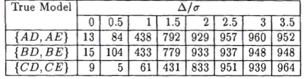
g ₅ _{61 431 833 951 939 964}

Table 6: The number of simulations out of 1000 where the correct true model

was identified, when the first two-factor interaction effect in the true model had a value of A and the second two-factor interaction effect had a value of

-A, following the addition of the augmenting runs ad and bd.

such as {ad, bd} and {bee, ace}, rather than the 12 pairs where three factors

change levels, such as {ad, ace} and {bd, bee}.

If <T is known to be 3.5, then for models to be regarded as consonant

with the true model the MSE needs to be less than 31.9. Of the 12 pairs

of eligible augmenting runs with only two factors changing levels, 10 would

have successfully identified {AD, AE} as the true model. The success of

this separation depends on the parameter values of the real two-factor in-teractions, the value of the standard deviation and also on which model is actually the true one. For example, for {ad, bd} the separation will be less

clear if {CD, CE} turns out to be the true model. This is demonstrated

by the simulation summarized in Table 6 giving, for various values of A/<r,

the number of simulations out of 1000 where the correct true Model was identified, when one of the real two-factor interaction effects had a value

of A and the other had a value of -A. If the models are not separated

after the initial augmenting runs then a further augmenting pair, giving less

separation if either {AD, AE} or {BD, BE} are the true models, should be

(14)

5. Conclusion

The orthogonal resolution IV fractional replicates yield the most efficient estimates of the main effects and are relatively simple to design and analyse. However in most cases the two-factor interactions are aliased in strings, and if one or more of these strings are significant then augmenting trials will be required.

The designs considered in this paper involve a small sacrifice in the efficiency of the estimation of the main effects. The major advantages are the fewer number of runs required and the ability to identify and estimate a small number of real two-factor interactions as long as the two-factor interactions do not take certain values. Even if they do, then it is possible to design an augmenting set, involving only two trials with up to five factors and three trials with up to nine factors that will enable the identification and estimation to be done.

References

BOX, G.E.P., HUNTER, W.G.,