Statistical Analysis and Computer Modelling of Volcanic Eruptions

(1)

Scholarship@Western

Electronic Thesis and Dissertation Repository

2-27-2014 12:00 AM

Statistical Analysis and Computer Modelling of Volcanic

Eruptions

Laura Anabelle Sanchez

The University of Western Ontario

Supervisor

Dr. Robert Shcherbakov

The University of Western Ontario Graduate Program in Geophysics

A thesis submitted in partial fulfillment of the requirements for the degree in Doctor of Philosophy

Follow this and additional works at: https://ir.lib.uwo.ca/etd

Part of the Geophysics and Seismology Commons, and the Volcanology Commons

Recommended Citation Recommended Citation

Sanchez, Laura Anabelle, "Statistical Analysis and Computer Modelling of Volcanic Eruptions" (2014). Electronic Thesis and Dissertation Repository. 1912.

https://ir.lib.uwo.ca/etd/1912

This Dissertation/Thesis is brought to you for free and open access by Scholarship@Western. It has been accepted for inclusion in Electronic Thesis and Dissertation Repository by an authorized administrator of

(2)

Modelling of Volcanic Eruptions

(Thesis format: Integrated Article)

by

Laura A. Sanchez

Graduate Program in

Geophysics Earth Sciences

A thesis submitted in partial fulfillment of the requirements for the degree of

Doctor of Philosophy

School of Graduate and Postdoctoral Studies The University of Western Ontario

London, Ontario, Canada

c

(3)

Volcanism is an important mechanism by which internal heat is transported to the

Earth’s surface and volcanic eruptions are the results of the dynamics of a complex

system and are characterized by non-trivial temporal correlations. Understanding

the processes involved in volcano formation and magma ascent are crucial to develop

better hazard assessment techniques. This study focuses on three main points: un-derstanding caldera formation in the solar system, investigating the global temporal

behaviour of volcanic eruptions and understanding the nonlinear interactions taking

place in the solid crust which lead to an eruption.

In chapter 2, I first examine the distribution of caldera diameters on Earth,

Mars, Io and Venus by performing a scaling analysis using the mean caldera

diam-eter as a scaling factor. I find that their probability densities can be described by

a universal distribution that can be approximated by a Generalized Extreme Value

distribution. This scaling implies that a similar process governs caldera formation throughout the solar system.

In chapter 3, I investigate the distribution of interevent times between eruptions

for active volcanoes on Earth. When rescaling the axis using the mean rate of

vol-canism, the distributions collapse into a single one, the log-normal distribution. This

scaling implies that the processes governing volcanic eruptions on Earth are similar

and are independent of the type of volcanism and location, which emphasizes the

importance of studying volcanism by modelling a universal behaviour.

In the last chapter, I take a modelling approach to study the interactions be-tween the magma and the crust. I define a lattice gas cellular automata model where

the magma is represented by discrete particles. In this model, magma propagates

through the crust and fracturing occurs until it reaches the top of the crust and an

eruption or a cascade of eruptions occur. I study the statistical behaviour of

erup-tions in the model and observe similar size and temporal behaviours that have been

(4)

Keywords: Statistical analysis, scaling, planetary calderas, volcanic eruptions,

cel-lular automata

(5)

This thesis is prepared in an integrated-article format and the following manuscripts

were written by Laura Sanchez.

1. Sanchez, L. and Shcherbakov, R. (2012), Scaling properties of planetary calderas

and terrestrial volcanic eruptions, Nonlin. Proc. Geophys., 19(6):585-593

2. Sanchez, L. and Shcherbakov, R. (2012), Temporal Scaling of Volcanic Eruptions,

J. Volcanol. Geotherm. Res., 247-248:115121, 2012

3. Sanchez, L. and Shcherbakov, R., A Cellular Automata to Model Magma-Crust

Interactions and Volcanic Eruptions, to be submitted

The data collection and analysis was performed by Laura Sanchez for manuscripts

1 and 2. The design of the model for manuscript 3 was done with Dr. Robert Shcherbakov. The work for these manuscripts was done under the supervision of Dr.

Robert Shcherbakov with financial support from the NSERC.

(6)

First, I would like express my deep appreciation to my supervisor Dr. Robert Shcherbakov. I am very grateful to have been part of his research group and I would like to thank him for his guidance, availability and patience with me during my PhD.

I would also like to express my gratitude to my committee members Dr. Gail Atkinson and Dr. Kristy Tiampo for their time and motivational words. I would also like to thank my examiners Dr. Gordon Osinski, Dr. Jean-Robert Grasso and Dr. M. Van De Wiel for taking the time out of their busy schedules to read and analyze my thesis.

I would have never been able to finish this endeavour without the precious help and support of the department staff members Marie Schell, Margaret Moulton, Katherine Johnson and Kevin Jordan. For all their advice and kind words, I am grateful.

I would like to thank my many reviewers who improved this thesis with ev-ery edit: Alexandra Pontefract, Marie Burford, Scott Colborne, Rachel Schwartz-Narbonne, Cassandra Marion, Jessica Stromberg. Your expertise of the English lan-guage was greatly appreciated!

For the stimulating discussions, I thank Dr. Pablo Gonzalez, Nelson Cho,

Pathikrit Bhattacharya and David Edey. And for the general support, all my col-leagues from office 1031, Andrea Prentice, Lola Wong (for introducing me to the pomodoro technique), Caitlin Atkinson, Meagan Pyper, Sonja Leal and all those I may have forgotten (you know who you are).

Lastly, I would like to thank my parents Irene and Pierre for their never failing support. I could never thank you enough for all the help you provided.

(7)

Abstract . . . ii

Co-Authorship Statement . . . iv

Acknowledgements . . . v

List of tables . . . viii

List of figures . . . x

1 Introduction . . . 1

1.1 Preamble . . . 1

1.2 Overview of Volcanism . . . 2

1.2.1 Planetary Volcanism . . . 2

1.2.2 Terrestrial Volcanism . . . 5

1.3 Statistical Modelling of Volcanic Processes . . . 10

1.4 Modelling of Volcanic Processes . . . 15

1.4.1 Numerical Models . . . 16

1.4.2 Cellular Automata Models . . . 18

1.5 Thesis Outline . . . 22

1.5.1 Chapter 2: Scaling Properties of Planetary Calderas . . . 22

1.5.2 Chapter 3: Temporal Scaling of Volcanic Eruptions . . . 23

1.5.3 Chapter 4: A Cellular Automata to Model Magma/Crust In-teractions and Volcanic Eruptions . . . 24

References . . . 25

2 Scaling Properties of Planetary Calderas . . . 34

2.1 Introduction . . . 34

2.2 Solar System Bodies . . . 37

2.3 The Earth . . . 44

2.4 Conclusions . . . 47

References . . . 48

(8)

3 Temporal Scaling of Volcanic Eruptions . . . 51

3.2 Volcanic Eruption Data . . . 53

3.3 Results and interpretation . . . 55

References . . . 70

4 A Cellular Automata to Model Magma-Crust Interactions and Vol-canic Eruptions . . . 73

4.2 The Model . . . 76

4.3 Results . . . 80

4.3.1 Model 1 (300×110) . . . 80

4.3.2 Model 2 (256×256) . . . 99

References . . . 133

5 Discussion and Concluding Remarks . . . 137

5.1 Caldera formation in the solar system . . . 138

5.2 Temporal behaviour of volcanic eruptions on Earth . . . 139

5.3 Modelling of volcanic eruptions . . . 139

5.4 Future work . . . 140

References . . . 142

Appendices A Tables of Volcanic Eruptions Time Series . . . 144

B Curriculum Vitae . . . 151

(9)

2.1 Summary of the data used for the planetary caldera analysis. Dnis the mean

diameter and An is the mean caldera area computed from the minimum

and maximum diameters assuming an elliptic shape for each planetary body except for the Earth where some caldera areas are estimated using the actual shape [Geyer and Marti, 2008]. The errors are given at 95% confidence

intervals. . . 41

2.2 The maximum values of the log-likelihood function (lnL) and the

corre-sponding values of the Akaike Information Criterion (AIC) for the model distribution functions considered to fit the rescaled distributions given in

Figure 2.2a.. . . 41

corre-sponding values of the AIC for the model distribution functions considered to fit a) the rescaled distributions given in Figure 2.2b and b) he rescaled

distributions given in Figure 2.4. k is the number of parameters for the

considered distribution. The values correspond to the fitting analysis

con-sidering only calderas/paterae with an area above 30 km2. . . 41

3.1 Summary of the eruption data used for the interevent time analysis of 26

prominent volcanoes. τn is the mean interevent time between eruptions

computed for each volcanic data set. The last column gives the time span of the eruption history considered for each volcano. The errors are given at

95% confidence intervals . . . 56

3.2 Summary of the eruption data used for the interevent time analysis for the

volcano types . . . 57

corre-sponding values of the Akaike Information Criterion (AIC) for the model distribution functions considered to fit a) the rescaled distributions given in Fig. (3.2), b) the rescaled distributions given in Fig. (3.3) and c) the

rescaled distributions given in Fig. (3.4). k is the number of parameters for

the considered distribution . . . 67

A.1 Summary of the eruption data used for the interevent time analysis for

the world regions . . . 144

A.2 Summary of the data used for the Alaska region with the number of eruptions, the time span, the mean interevent time and the type of

volcano. . . 144

(10)

A.3 Summary of the data used for the Aleutian islands with the number of eruptions, the time span, the mean interevent time and the type of

volcano. . . 145

A.4 Summary of the data used for Central America with the number of eruptions, the time span, the mean interevent time and the type of

volcano. . . 145

A.5 Summary of the data used for Iceland with the number of eruptions,

the time span, the mean interevent time and the type of volcano. . . 146

A.6 Summary of the data used for Indonesia with the number of eruptions,

A.7 Summary of the data used for Japan with the number of eruptions,

A.8 Summary of the data used for Kamchatka with the number of erup-tions, the time span, the mean interevent time and the type of volcano. 148 A.9 Summary of the data used for New Zealand with the number of

erup-tions, the time span, the mean interevent time and the type of volcano. 149 A.10 Summary of the data used for South America with the number of

eruptions, the time span, the mean interevent time and the type of

volcano. . . 149

A.11 Summary of the data used for the eruption of major calderas on Earth with the number of eruptions, the time span and the mean interevent

time. . . 150

(11)

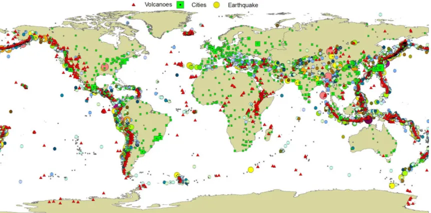
1.1 Simplified map presenting the location of major cities, earthquakes and

volcanoes. (modified after www.USGS.gov) . . . 3

1.2 Sketch of the magma plumbing system. The magma chamber is located at

a depthH from the surface and the pressure within the chamber is a

com-bination of the pressure due to the host rock P1(H) and the overpressure

generated by the input of magma or the increase in gas content in the

cham-ber ∆Pc. The eruption exit pressure is a combination of the atmospheric

pressure Pa and the excess pressure in the vent ∆Pe. The lithostatic

pres-sure around the chamberPL(z) is a function of depth and the density of the

host rockρr [Jaupart, 2000]. . . 7

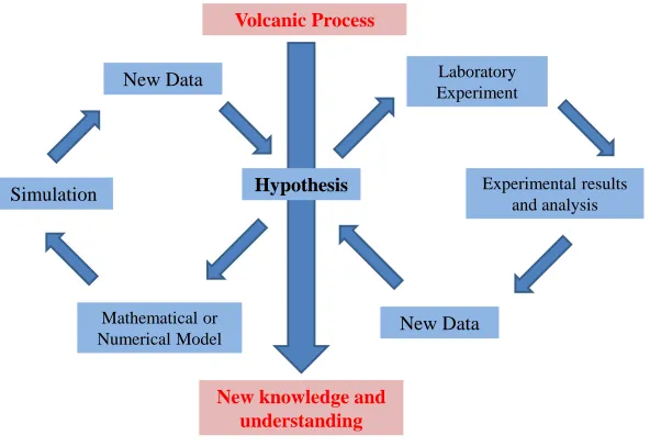
1.3 Schematic steps of the use of experimental and numerical/mathematical

modeling to validate hypotheses on volcanic processes . . . 16

1.4 Example of the evolution of the Wolfram CA from rule 30. The upper part

displays the evolution rules for each possible configuration at time t (from

www.mathworld.wolfram.com) . . . 19

1.5 Power-law behaviour of the magnitude-frequency of Holocene eruptions [Simkin,

1993] . . . 21

2.1 Distributions of caldera sizes for the Earth, Venus, Mars and Io. a) Caldera

diameters in km, b) Caldera areas in km2. . . 39

2.2 Rescaled caldera/paterae distributions for Earth, Mars, Venus and Io

ac-cording to Eq. (2.1): a) rescaled diameters, with the mean diameter Dn

computed for each planetary body (Table 2.1). The solid curve is a fit to the rescaled distributions and is given by the GEV distribution, Eq. (2.2),

withθ= 0.22±0.06, µ= 0.64±0.04, and σ = 0.42±0.03; b) rescaled

ar-eas, with the mean areaAn computed for each planetary body (Table 2.1).

The solid curve is a fit to the rescaled distributions and is given by the

GEV distribution, Eq. (2.2), with θ = 0.84±0.11, µ = 0.26±0.03, and

σ= 0.30±0.03 . . . 42

2.3 Probability density functions of caldera areas for three separate crustal types

on Earth. . . 45

2.4 Rescaled caldera areas distributions for the three crustal types according to

Eq. (2.1) with the mean areaAncomputed for each crustal type (Table 2.1).

The solid curve is a fit to the rescaled distributions and is given by the

GEV distribution, Eq. (2.2), with θ = 0.94±0.16, µ = 0.22±0.04, and

σ= 0.28±0.05. . . 46

(12)

3.1 Probability density functions of interevent times for the 26 volcanoes on

Earth with the largest eruptive history . . . 57

3.2 Rescaled interevent time distributions for the 26 individual active volcanoes

according to Eq. (3.1) with the mean interevent timeτn computed for each

volcano (Table 3.1). The solid curve is a fit to the rescaled distributions and

is given by the log-normal distribution, Eq. (3.2), with µ = −0.66±0.05

and σ = 1.14±0.04. The errors on the parameters are given at the 95%

confidence interval assuming a log-normal distribution. The error bars are

not displayed for the sake of clarity . . . 59

3.3 The combined rescaled interevent time distributions of groups of volcanoes

belonging to 9 different regions. Each individual volcano sequence was first rescaled with the mean interevent time and only after that the distributions were constructed. Data collapse was observed similar to the one shown in Figure 3.2. The solid curve is a fit to the rescaled distributions and is given

by the log-normal distribution withµ=−0.70±0.05 andσ = 1.23±0.03.The

errors on the parameters are given at the 95% confidence interval assuming

a log-normal distribution . . . 60

3.4 The combined rescaled interevent time distributions of volcanoes grouped

by type. Each individual volcano sequence was first rescaled with the mean interevent time and only after that the distributions were constructed. Data collapse was observed similar to the one shown in Figure 3.2. The solid curve is a fit to the rescaled distributions and is given by the log-normal

distribution with µ=−0.70±0.04 and σ = 1.24±0.03. The errors on the

parameters are given at the 95% confidence interval assuming a log-normal

distribution . . . 61

3.5 The combined rescaled interevent time distributions of groups of volcanoes

belonging to different regions. Each individual volcano sequence was first rescaled with the mean interevent time and only after that the distributions were constructed. The lower magnitude cutoff of eruptions was used: a)

VEI ≥ 1.0; b) VEI ≥ 2.0; c) VEI ≥ 3.0. The solid curve is a fit to the

rescaled distributions and is given by the log-normal distribution with a)

µ=−0.70±0.05 andσ= 1.23±0.04; b)µ=−0.67±0.06 andσ= 1.22±0.04;

c) µ = −0.59±0.15 and σ = 1.27±0.11. The errors on the parameters

are given at the 95% confidence interval assuming a log-normal distribution.

The error bars are not displayed for the sake of clarity . . . 62

3.5 Continued. . . 63

(13)

3.6 Rescaled interevent time distributions for the 26 individual volcanoes

ac-cording to Eq. (1) with the mean interevent timeτnfor each volcano. Lower

magnitude cutoffs of eruptions were used: a) VEI≥1.0; b) VEI≥2.0. The

solid curve is a fit to the rescaled distributions by the log-normal

distribu-tion with a)µ=−0.68±0.08 andσ = 1.20±0.06; b)µ=−0.68±0.07 and

σ= 1.18±0.06. . . 65

4.1 Different possible configurations for particle positions in the HPP model for

the cases of 4,3 and 2 particles on a node (a,b,c,d). Schematic view of the

2D lattice with the distinction between the magma chamber and the crust (e) 79

4.2 Collision and propagation rules for the different configuration of particles

on the lattice . . . 79

4.3 Propagation directions for model 1 (left) and model 2 (right). . . 80

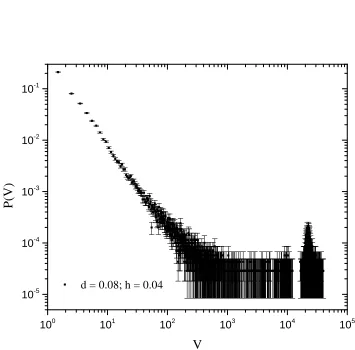
4.4 Example of the frequency-size distribution of eruptions for d = 0.08 and

h= 0.04. We note the peak at 3×104 . . . 83

4.5 Truncated power-law fit of the frequency-size distribution for the size range

V ∈[30,1000] withα= 1.36±0.03. . . 84

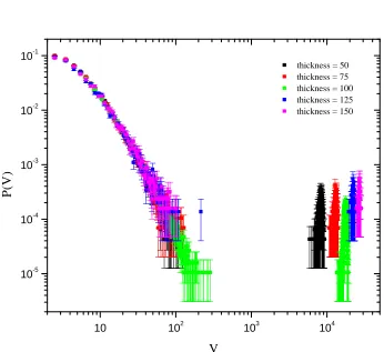
4.6 Frequency-size distributions of eruptions ford= 0.5 andh= 0.2 and varying

thickness of the system. . . 85

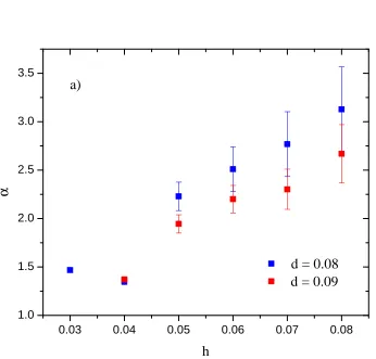
4.7 Variation of the power-law exponentα withh for small values of d. . . 86

4.8 Variation of the power-law exponentα withh for large values of d(b). . . 87

4.9 Frequency size distributions of eruptions forh= 0.5 and large values of d. 88

4.10 Truncated power-law fit of the frequency-size distribution for d= 0.9 and

h= 0.5 for the size rangeV ∈[7,100] with α= 4.36±0.72. . . 89

4.11 Example of the log-normal regime for the distribution of eruptions interevent

times ford= 0.5 andh= 0.2. . . 92

4.12 Truncated log-normal fit of the distribution for the time rangeτ ∈[60,300]

withµ= 3.48±0.61 and σ = 0.54±0.14 . . . 93

4.13 Example of the exponential regime for the distribution of eruptions

in-terevent times ford= 0.5 andh= 0.4. . . 94

4.14 Truncated exponential fit of the distribution for the time rangeτ ∈[50,200]

withλ= 26.27±2.11. . . 95

4.15 Example of the power-law regime for the distribution of eruptions interevent

times ford= 0.5 andh= 0.6. . . 96

4.16 Truncated power-law fit of the distribution for the time rangeτ ∈[30,300]

withα= 1.51±0.05 (b) . . . 97

4.17 Phase diagram representing the best model to describe the interevent data

for varying values ofdand h. . . 98

4.18 Truncated log-normal fit of the distribution for the size rangeV ∈[100,10000]

withµ= 3.52±0.58 and σ = 1.46±0.17 (model 2) . . . 100

(14)

4.19 Truncated power-law fit of the distribution for the size rangeV ∈[100,10000]

withα= 1.96±0.03 (model 2) . . . 101

4.20 Phase diagram representing the best model to describe the frequency-size

distributions from model 2 for varying values ofdandh. The label ”other”

corresponds to cases where the 3 distributions considered were not a good fit102

4.21 Phase diagram representing variations in theµparameter for the truncated

log-normal fit of the size distribution of events forC= 0.6 . . . 103

4.22 Phase diagram representing variations in theσ parameter for the truncated

log-normal fit of the size distribution of events forC= 0.6 . . . 104

4.23 Phase diagram representing variations in theαparameter for the truncated

power-law fit of the size distribution of events forC = 0.6. . . 105

distributions from model 2 for varying values ofdand h forC= 0.55 . . . 106

distributions from model 2 for varying values ofdand h forC= 0.65 . . 107

4.26 Truncated exponential fit of the distribution for the time rangeτ ∈[300,10000]

withλ= 215.4±11 . . . 109

4.27 Truncated log-normal fit of the distribution for the time rangeτ ∈[100,10000]

withµ= 3.53±0.22 and σ = 1.42±0.07 . . . 110

4.28 Truncated power-law fit of the distribution for the time rangeτ ∈[100,10000]

withα= 1.92±0.02 . . . 111

4.29 Phase diagram representing the best model to describe the interevent

dis-tributions from model 2 for varying values ofdand h forC= 0.60 . . . . 112

log-normal fit of the size distribution of events forC= 0.6. . . 113

log-normal fit of the size distribution of events forC= 0.6. . . 114

4.32 Phase diagram representing variations in theλparameter for the truncated

exponential fit of the size distribution of events forC= 0.6. . . 115

power-law fit of the size distribution of events forC = 0.6. . . 116

4.37 Truncated exponential fit of the distribution for the time ranget∈[100,10000]

withλ= 163.5±6.9 . . . 121

4.38 Truncated log-normal fit of the distribution for the time ranget∈[100,10000]

withµ= 5.7±0.18 and σ= 0.81±0.13 . . . 122

(15)

4.39 Truncated power-law fit of the distribution for the time ranget∈[200,10000]

withα= 4.23±0.75 . . . 123

4.40 Phase diagram representing the best model to describe the duration

distri-butions from model 2 for varying values of dandh forC = 0.60 . . . 124

log-normal fit of the distribution of durations forC = 0.60. . . 125

log-normal fit of the distribution of durations forC= 0.60. . . 126

power-law fit of the distribution of durations for C= 0.60. . . 127

(16)

Chapter 1 Introduction

1.1 Preamble

Volcanic processes are the surface expression of a planetary body’s internal activity. They constitute an efficient mechanism to dissipate internal heat. Volcanism is or was

present on rocky planetary bodies in our solar system such as Earth, Mars, Venus,

Mercury, the Moon, Io and several other planetary satellites [Wilson, 2009, Prockter

et al., 2010]. On Earth, volcanic eruptions constitute a major natural hazard and

with currently around 500 million people living in the vicinity of active volcanoes,

the potential effects of an eruption on population and goods is becoming greater every

day [Kusky, 2008] (Figure 1.1 shows a World map of the major cities and the location

of volcanoes and earthquakes). Large explosive eruptions can have local effects such

as land destruction through pyroclastic flows, but also global environmental effects through the dissemination of ashes and aerosols in the atmosphere from eruption

plumes [Gilbert and Sparks, 1998].

Volcanoes are complex dynamical systems and the interactions between the

magma and the host rock occurring within the edifice result in eruptions. These

nonlinear interactions lead to the stochastic character of eruptions. Volcanic processes

have been extensively studied through field and numerical analysis providing us with

some quantitative understanding of the main physical mechanisms. However, our

current knowledge remains insufficient to explain and forecast the temporal behaviour

of eruptions. The deterministic character of the modelling fails at reproducing the temporal patterns observed. Therefore, understanding the mechanisms responsible

for volcano formation and the nonlinear interactions that lead to eruptions alongside

with being able to reproduce the observed temporal patterns are crucial steps in the

field of volcanology and hazard assessment.

This thesis focuses on three primary areas of concern:

• Understanding caldera formation and evolution in the solar system using

(17)

• Investigating the global temporal behaviour of volcanic eruptions on Earth,

• Understanding the nonlinear interactions taking place in the solid crust which

lead to an eruption.

In order to investigate similarities in volcanic processes throughout the solar

system, we compare the size distribution of volcanic features on Earth and other

planetary bodies to infer common formation mechanisms. Particularly, we investigate

the statistical properties of circular shaped depressions called calderas on Earth, Mars,

Venus and Io. This type of feature is associated with the collapse of the volcanic edifice

into a drained or partially drained magma chamber and can be used as a proxy to estimate the potential size of eruptions [Lipman, 2000]. Our goal is to further our

understanding of formation and evolution mechanisms for planetary landforms.

The current knowledge on eruption processes, paired with the numerous

moni-toring tools available for volcano surveillance and historical records allow us to have

access to a large wealth of data. Utilizing these data through statistical analysis is

a powerful approach to determine temporal and spatial patterns in volcanic activity.

This thesis relies on statistical approaches investigating the temporal behaviour of

eruptions throughout the World [Siebert and Simkin, 2002-].

Using a computer modelling approach, we study the complex magma/crust interactions in volcanic settings. More specifically, a cellular automaton model is

used in order to reproduce the statistics observed in the empirical eruption data for

volcanoes on Earth. The goal is to reproduce the statistical behaviour of eruptions

using the least amount of parameters to capture essential physical mechanisms of

volcanic eruptions.

1.2 Overview of Volcanism

1.2.1 Planetary Volcanism

Volcanism is an inevitable consequence of planetary differentiation and crustal

gener-ation by magmatic processes. The heat present in the solar system planetary bodies

is mostly generated by accretional energy and the decay of short and long lived

ra-dioactive nuclides. The release of planetary body’s internal energy creates internal

(18)

Figure 1.1: Simplified map presenting the location of major cities, earthquakes and volca-noes. (modified after www.USGS.gov)

towards the surface, which leads to volcanism. Tidal stresses induced on satellites by the presence of a large body is also considered a considerable source of heat that

can enable volcanism. Space exploration has allowed remote access to most planetary

bodies in our solar system. While it is difficult to make any kind of observations

below the thick atmosphere of the gas giants, satellite observations from terrestrial

planets have indicated the presence of radioactive elements. Planetary exploration

has also directly shown that volcanism is or was operational on other solar system

bodies such as the Moon, Venus, Mars, Mercury, Io, and several other planetary

satel-lites [Wilson, 2009, Prockter et al., 2010]. Volcanic processes are therefore a typical

heat dissipation mechanism on terrestrial planetary bodies. The resultant landforms depend on parameters such as the bulk chemistry of the parent magma, the nature

of fractures and feeders and their study can lead to a better understanding of the

planet’s internal dynamics.

Volcanism on the Moon is mostly characterized by large basaltic flows called

mares. In its early history, portions of the mantle experienced partial melting and

the melt was lead to rise through cracks and fractures created by the large impact

craters and basins at the surface. The large flows filled those craters and ended up

covering around 20% of the surface of the Moon [Spudis, 2000]. When smaller volumes

(19)

such as domes and cones. Their shape depends on the style and rate of eruption rather than on the magma composition [Head, 1976, Head and Gifford, 1980]. Some

pyroclastic materials were collected from the surface of the Moon by the Apollo 15 and

17 missions, suggesting that some lava fountain type of eruptions may have occurred

in the satellite’s past [Spudis, 2000].

One of the solar system’s planetary bodies that is the closest to the Earth as

far as composition, density and size is Venus. Because of those analogies, the thermal

evolution of Venus and the Earth is similar and they both experienced extensive

vol-canic activity. However, the style of volcanism on Venus is very different from the one

observed on Earth. Where mantle convection and plate tectonics are the main causes for volcanic activity on Earth, major resurfacing events involving flood basalts seem

to be taking place on Venus [Nimmo and McKenzie, 1998]. The centres for volcanic

activity seem to be scattered at the surface, similarly to intraplates volcanic centres

on Earth [Wilson, 2009]. The type of features present on Venus include small and

large shields, lava flows, dike swarms and flood basalt provinces. Some do not have

terrestrial analogs such as coronae which are circular features exhibiting concentric

radial fractures [Crumpler and Aubele, 2000], arachnoids (named after their

resem-blance to spider webs) and novae. These unusual features might be the product of

how differently the Venusian crust handles deformation [Parfitt and Wilson, 2009]. Mars is one of the terrestrial planets in our solar system that exhibits great

geological diversity alongside with the Earth. No active plate tectonics has been

observed on this body as there is no evidence of active ridge and trench systems.

The planet is divided into two main areas: the highlands, covered with extensive lava

flows; and the lowlands, where volcanic plains cover most of the surface [Wilson, 2009].

Two volcanic provinces contain most of the erupted volcanic materials: Tharsis and

Elysium. In these areas, large shield volcanoes can be observed, including the highest

mountain in the solar system: Olympus Mons [Parfitt and Wilson, 2009]. These large

shields are the result of basaltic flows and can be compared to intraplate volcanoes on Earth. Cones of various sizes are also present on Mars and have been compared

to cinder cones on Earth [Frey and Jarosewich, 1982].

Mercury is the smallest planet in our solar system and also the densest. This

very high density reflects the presence of a large iron core (compared to the size of the

planet) which could potentially provide a considerable heat source to enable volcanism

(20)

of Messenger, our knowledge of the surface of the planet came from images made by Mariner 10 during its fly-bys in 1974. Messenger was able to image an additional

21% of the planet and the hypothesis about the volcanic nature of intercrater plains

[Strom et al., 1975] was confirmed. Volcanic vents were observed and identified as

the source for effusive eruptions and the formation of shield volcanoes and lava flows

[Head et al., 2009]. Some evidence for explosive volcanism was also gathered from

the images [Prockter et al., 2010].

Io is one of Jupiter’s satellites and is the most volcanically active planetary body

in the solar system. Unlike most of the other bodies, the source for internal heating

for Io comes from the colossal tidal force that Jupiter applies on its satellite. More than 300 vents have been identified at the surface and no signs of plate tectonics have

been detected. Silicate volcanism seems to be the main type of volcanism present

and the identified hot spots exhibit two types of activity: persistent and sporadic

[Lopes-Gautier et al., 1999]. The main types of feature present at the surface are

lava flows, lava fountains, high mountains and an analog to terrestrial caldera called

paterae [Radebaugh et al., 2001].

Comparative planetology aims at comprehending the physical factors governing

the shape of planetary landforms as well as the styles and patterns of eruption. Past

studies have attempted to compare volcanic structures on Earth to similar features on other planetary bodies with some success. Similarities have been found between

Martian cones and cinder cones on Earth [Frey and Jarosewich, 1982] and also

be-tween small Venusian domes, shields and cones and terrestrial sea floor volcanoes

[Smith, 1996, Bulmer and Wilson, 1999]. Because of the relationship between caldera

diameter and magma chamber dimensions and depth, the comparative study of

plan-etary calderas constitute a great tool to gain a better understanding of planplan-etary

subsurfaces [Wood, 1984].

1.2.2 Terrestrial Volcanism

Volcanic eruptions on Earth are the result of complex interactions between magma

(molten rock) and the crust, and volcanoes are non uniformly distributed across the

surface, being primarily located at plate boundaries (subduction zones or mid-ocean ridges, see Figure 1.1). Around subduction zones, hydration of the mantle is caused

(21)

and subsequent rise of magma into the crust. At divergent margins, decompression of the mantle under a thinning plate enables partial melting. Active volcanism can also

be found in the middle of tectonic plates and is characterized by hot spots volcanoes.

In this case, melting is allowed by the presence of high temperature zones deeper in

the mantle. A plume is generated and feeds the volcanoes at the surface.

Within the crust and the mantle, magma rises due to density differences. When

a depth where the magma is neutrally buoyant is reached, the latter accumulates

forming a continuous body called a magma chamber. The depth of magma chambers

ranges from about 2 to 10 km, depending on the magma composition (Pinkerton et al.

[2002] and references therein). Once in this storage area, the magma starts to evolve. Cooling will bring its temperature below the liquidus, allowing successive minerals

to form. This process is referred to as fractional crystallization [Parfitt and Wilson,

2009]. As the magma cools and crystallizes in the chamber, volatiles such as water

and halogens will appear in the residual melt, according to the magma composition.

When their concentration reaches a saturation level, gas is exsolved to form bubbles

in the chamber. This process induces a sudden reduction in density, which increases

the buoyancy of the material in the magma chamber. This presence of bubbles is

also responsible for a pressure increase in the magma chamber. Once this pressureP

becomes larger than the lithostatic pressure P_L by an amount larger than the value

of the tensile strength (maximum amount of stress the material can withstand before

failure) of the chamber walls, the creation of cracks, or dykes, above the chamber

is possible and the magma starts rising [Blake, 1981]. This gas bubbles formation

process, alongside with the addition of new magma in the chamber are considered as

two of the main causes for initiating eruptions. Figure 1.2 presents a schematic view

of the magmatic plumbing system.

Scandone et al. [2007] proposed a conceptual model to describe magmatic

pro-cesses. They divided the magma system into four different regions. The supply

sys-tem is located at the crust/mantle boundary and provides the primary deep source of magma. For small eruptions, this area is not involved directly in the eruption

process. The intermediate storage system is located at mid to shallow depths in the

crust and constitute what we previously defined as the magma chamber. There, the

magma can stop or rise due to density differences and will start to cool and evolve.

The third region is the transport system. As previously described, when the magma

(22)

Figure 1.2: Sketch of the magma plumbing system. The magma chamber is located at

a depth H from the surface and the pressure within the chamber is a combination of

the pressure due to the host rock P1(H) and the overpressure generated by the input of

magma or the increase in gas content in the chamber ∆Pc. The eruption exit pressure is a

combination of the atmospheric pressurePa and the excess pressure in the vent ∆Pe. The

lithostatic pressure around the chamberPL(z) is a function of depth and the density of the

(23)

local stress field changes and density unbalance that allows the magma to propagate through a fracture system. The last component of Scandone et al. [2007]’s system is

the eruptive system, a shallow region in the crust from where the magma is erupted.

Depending on the magma composition and therefore the volatile content (H₂O, CO₂,

SO₂, H₂S) in the chamber, different styles of eruptions will be initiated.

The overpressure in the magma chamber initiated by the input of new magma

or the increase in volatile content leads to the formation of dikes. Dikes are hydraulic

fractures within the crust that allow the magma to rise from one reservoir to another,

and ultimately to the surface [Tait and Taisne, 2013]. Almost all eruptions are

sup-plied with magma from the chamber to the surface through dikes. The propagation and evolution of dikes depend on the stress state surrounding the volcano

[Gudmunds-son, 2006]. Understanding the formation, propagation and arrest of dikes between the

magma chamber and the surface is therefore one of the requirements to understand

the temporal pattern of eruptions. Theoretical models have considered the effects of

overpressure or buoyancy in an existing crack. The flow in the magma filled crack can

be described using fluid dynamics non linear equations [Lister, 1990]. Many analogue

experiments have also been carried out to link theoretical models of dike propagation

and geological observations. Acocella et al. [2008] investigated the dike patterns of

Somma-Vesuvius and Etna using a laboratory experiment. The crust and magma were modelled using respectively gelatin and water. The water was injected in the

cone and the formation of dikes was studied. The results of that experiment showed

that, in that case, dikes at the surface exhibited a radial pattern while tangential

and oblique dikes were observed at depth. These results have implications for the

prediction of the location of future eruptions on the volcanic edifice. As stated

be-fore, the stress state within the volcano influences the formation and propagation of

dikes. Many studies using analytical models have investigated the stress field around

a volcano by considering the host rock as a homogeneous and isotropic system with

an elastic behaviour ([Gudmundsson, 2006] and references therein).

Volcanoes can exhibit explosive and effusive activity. The type of eruption

de-pends largely on the magma’s silica content. Silica rich magmas can contain up to 6%

of water and the eruptions associated will be characterized as explosive. With a high

silica content comes a large volume of gas bubbles in the chamber. When this volume

is large enough, a continuous phase will be initiated from the bubbles connecting

(24)

ex-plosive eruption can be manifested by several outputs. Strombolian eruptions exhibit small and discrete explosions of ashes, gas and magma. Hawaiian eruptions display

in-tense and near continuous fire fountains [Vergniolle and Mangan, 2000], while Plinian

eruptions are infrequent but extremely explosive and sustained and characterized by

stable eruption clouds [Cioni et al., 2000]. As stated before, fragmentation is one

of the processes responsible for explosive eruptions and has therefore been

exten-sively studied. This mechanism corresponds to the transformation process of bubbly

magma into gas-pyroclast dispersion [Papale, 1999]. Laboratory experiments have

been designed to study the mechanisms responsible for bubble nucleation,

accelera-tion of the flow and the process of fragmentaaccelera-tion. Mader et al. [1994] proposed to

simulate explosive eruptions by generating supersaturation of CO₂ in a liquid phase

(water in this case). Phillips et al. [1995], used a gum-rosin acetone solution to

sim-ulate the conduit flow that leads to fragmentation. Both these models were able to

demonstrate that decompression in a supersaturated liquid is the starting point of

the fragmentation process. Going further in the investigation of the fragmentation

process, Stix and Phillips [2012] studied the role of the speed of pressure changes

in the process of fragmentation. Using the same gum rosine acetone system, they

showed that fragmentation is induced by only fast decompression conditions.

Basaltic magma, with a significantly lower silica content, will result in effusive eruptions. The main products of basaltic eruptions are lava flows, lava fountains

and the creation of volcanic fields. When the silica content increases, the magma

becomes more viscous and blocky flows and domes are generated. Volcanoes can

display different types of activity during their eruptive history. During an eruption,

the degree of explosivity will decrease with time. The volatile rich magma is mostly

concentrated at the top of the chamber and erupts first, leaving the magma available

for the rest of the eruption poor in volatiles. The reduced pressure in the chamber

due to the loss of magma from the eruption also has an effect on the ascent velocity,

which also controls the explosivity of the eruption [Pinkerton et al., 2002]. There seem to be a transition between effusive and explosive activity when a critical ascent

rate of 0.2 ms−1 is reached [Rutherford and Gardner, 2000].

The different styles of volcanic activity give birth to different volcanic

land-forms [Lockwood and Hazlett, 2010]. Here, we only overview the most common and

prominent types of features. Shield volcanoes are the product of effusive activity

(25)

such structures have a very low viscosity and are initiated at shallow depth. Compos-ite volcanoes, or stratovolcanoes, are the result of a complex eruptive history. The

edifice is built from the deposition of multiple eruptive layers. Cinder cones are a

smaller volcanic feature resulting from Strombolian type, basaltic eruptions. When

large eruptions occur, the drained magma chamber can collapse and form a

multi-kilometre wide, quasi-circular depression called a caldera [Lipman, 2000]. This type

of feature can be observed on top of shield or stratovolcanoes.

There are approximately 1500 volcanoes on land on Earth [Tilling, 1989]. The

most active volcanoes are currently extensively monitored using a wide variety of

tools such as seismic sensors, GPS measurements, to mention a few. Historical data are also very rich in information and allow us to have access to a significant amount

of data on the temporal evolution of eruptions. This wealth of data allows us to study

volcanic processes from a statistical point of view in order to identify patterns in their

activity.

1.3 Statistical Modelling of Volcanic Processes

Statistical analysis is a powerful tool to study the characteristics of natural processes and to infer the physical mechanisms underlying those processes. One of the first

statistical analysis carried out on volcanic data was performed by Wickman [1966] on

Hawaiian volcanoes. One of the main statistical models used to describe the observed

temporal patterns of eruptions was the Poisson process.

A homogeneous Poisson process is a mathematical model that describes a series

of random events. Events in that case are stationary and independent from each other

[Ho, 1991]. The main characteristics of such a model are the following [Cox and Lewis,

1966]:

• The probabilities of an event happening or not, do not change in time, and

therefore, the time series does not display a trend.

• Two events have negligible chances of happening together.

• The probability of an event happening at time t+h is independent on what

happened at time t. The probability of an event happening at t+h does not

(26)

When studying natural hazards time series, one useful characteristic to

inves-tigate is the distribution of intervals between events, or interevent times τ. The

interevent times for a homogeneous Poisson process are exponentially distributed

and the distribution is characterized by the parameter λ. This parameter represents

the rate of events, or how many events can occur per unit time. In this case, λ is a

constant. The events are independently distributed and occur at a constant average

rate.

The hypothesis of volcanic eruptions behaving as a Poisson process has been

tested on a wide range of datasets. As previously stated, Wickman [1966] investigated

the temporal behaviour of Mauna Loa and Kilauea volcanoes. He found that the eruptive activity of Mauna Loa can be approximated by a Poisson process but that

the activity of Kilauea showed a non-constant event rate. Reyment [1969] studied

the activity of 3 Japanese volcanoes, Etna, 3 Indonesian volcanoes and Mauna Loa.

He was able to show the random behaviour of Mauna Loa and Bromo volcanoes. His

study led him to conclude that some eruption time series could be approximated by

a Poisson process but that this model was not universal for all volcanoes.

The activity of Stromboli volcano was examined through the eruption sequence

of 3 different vents [Settle and Mcgetchin, 1980]. It was found that the interevent

time distributions for 2 of the 3 vents could be fitted by an exponential distribution, and therefore their activity could be modelled by a Poisson process. The eruption

mechanism at the remaining vent could be characterized by a normal (Gaussian)

process. A correlation was observed between the temporal behaviour of vents 2 and

3 with vent 1. This dependency suggested that vents 2 and 3 were directly connected

to the magma reservoir beneath vent 1.

Another study of the activity of the Hawaiian volcanoes defined the interevent

times of volcanic events as the time elapsed from one eruption onset to the other,

Klein [1982] investigated flank and summit eruptions. Again, a Poisson process was

concluded to be a good fit, despite some departure from the model was observed for the distribution of interevent times between large eruptions and eruptions of any size

following them. This discrepancy was explained by the finite character of the magma

supply in the volcano. De la Cruz-Reyna [1991] investigated the temporal patterns

of global volcanic activity. It was found that for large eruptions, the distribution

of interevent times between eruptions could be modelled by a homogeneous Poisson

(27)

of energy while releasing it in small amounts at a constant rate.

In all of the aforementioned works, the hypothesis of volcanic events being a

series of independent random events has been validated but it was also often noticed

that this model was not universal for all of the datasets considered. The introduction

of the non-homogeneous Poisson process as a generalization of the model has allowed

some of the behaviours to be better explained. A non-homogeneous Poison process, or

time-dependent Poisson process, satisfies the same assumptions than a homogeneous

Poisson process, but λ is now a function λ(t) of time. When the randomness of

events implies that several processes are combined to trigger eruptions, having a

non-homogeneous Poisson process implies that the balance between those processes changes with time.

Ho [1991] tested the non-homogeneous model on 5 individual volcanoes. In that

study, he considered an eruptive rateλ(t) such asλ(t) =βθ−βtβ−1 whereβ andθ are

constant parameters and t is the time since a predefined origin. Bebbington and Lai

[1996a] argued that this approach was unsatisfactory and proposed a more general

approach. They proposed a Weibull renewal model to describe the occurrence of

vol-canic eruptions on New Zealand volcanoes. A renewal process comprises interevent

times that are identically and independently distributed that have a common

distri-bution D. For the homogeneous Poisson process, D is an exponential distribution.

For the Weibull renewal process, used by Bebbington and Lai [1996b],Dis a Weibull

distribution. This type of renewal model was used in order to issue prediction on the

eruptive activity of Mount Vesuvius, whereDwas defined as Gamma distribution [Ho,

1992]. Using this very same non-homogeneous Poison process approach, Dzierma and

Wehrmann [2010] investigated the interevent time distributions for volcanoes in the

south Chile volcanic zone using several distributions such as the Weibull, the

log-logistic and the exponential distributions to describe D. All the examples show that

the non-homogeneous Poisson process can be successful at describing eruption time

series. The nature ofDseems to be different depending on the volcanoes considered.

Other methods have been developed with the same goal of fitting the interevent times

distribution of eruptions, such as a mixture of exponential distributions

[Mendoza-Rosas and De la Cruz-Reyna, 2009].

When examining the temporal patterns with the goal of mitigating volcanic

risks, it is important to consider the return period of large eruptions since they tend

(28)

tail of the distributions describing their probability of occurrence [Albeverio et al., 2006]. The statistics of extremes have been originally developed by Gumbel [1958]

and the goal is to gather as much information as possible on the temporal and spatial

distributions describing these large events. Being able to characterize the statistical

distribution of extreme events is one of the biggest challenges that researchers have

been trying to overcome. The main goal is to predict the size of the next largest

event, or the probability that the largest event will occur in a certain time window

and at a certain location [Gumbel, 1958]. Investigating the statistical behaviour of

the distribution times between two consecutive extremes, has been proven successful

at characterizing the temporal properties that can be used to predict such events [Altmann and Kantz, 2005].

Pyle [1998] used the rank-ordering method in order to define the likely size of

extreme volcanic eruptions. This method was introduced in statistics by Gumbel

[1958] and has been applied to a large number of problems since then. The concept

of the method is simple. The sizes of eruptions are ordered where the largest event

has the first rank, the next largest the second and so on. The analysis is done by

plotting the size of the events versus their rank [Pyle, 1998]. One of the reasons for

carrying out this analysis was to try and place an upper limit on the size of future

extreme eruptions. For the study, several datasets were used: data for large volcanic eruptions since A.D 1815 and data from the Taupo volcano in New Zealand for the

last 25 000 years [Pyle, 1998]. This method allowed them to predict the size of the

next largest events and the longest time interval between events for the catalogues

considered.

Coles and Sparks [2006] applied extreme value statistics to a 2000-year eruption

catalogue. The goal of the analysis was to determine the parameters associated with

intensity function λ(t), and ultimately deriving the return period rassociated with a

certain magnitudem: r(m). This analysis raised the issue of the choice of a magnitude

threshold when using extreme value statistics. If a high threshold is chosen for the analysis, the results will be truly representative of extreme events but the quality of

the statistics will be poor since extremes are, by definition, rare. On the other hand,

choosing a lower threshold will increase the quality of the statistics but the events

sampled are not all extremes events. In addition, the fact that the catalogue used

for this study only covers the last 2000 years makes it difficult to make inferences

(29)

[2010] applied the same method to a new database of Holocene explosive volcanism. They showed that the model, due to a large amount of under reporting in the data,

was predicting maximum eruption magnitudes that were too small because of the

sampling biases. The likely explanation is that the available data only sample the

high end of ”ordinary” eruptions (characterized as Plinian) and that the mechanism

behind ”super eruptions” is different. The method used in that study was only able

to predict recurrence rates for the upper limit of Plinian-type eruptions but not for

the super-eruptions.

We have provided an overview of the type of common statistical analyzes that

have been done on volcanic eruptions. Like many natural hazards, eruptions have also been considered as a self-organized process [Grasso and Bachelery, 1995]. Such a

process is characterized by a slowly driven dynamical system which organizes itself in

a critical state. Once this state is reached, dissipation occurs in the form of avalanches

of all sizes that are regular in time, but not periodic [Bak et al., 1988]. One example

of this kind of system is described by the sandpile model: when constantly adding

sand grains to a small sandpile, small and big avalanches will rapidly form in order

to decrease the local slope whenever they reached a critical angle. The frequency

size distribution of those avalanches is described as a power-law in the case of a

self-organized system [Bak et al., 1988]. The distribution of magnitudes and/or Volcanic Explosivity Index (VEI) of volcanic eruptions, displays scale-invariant characteristics

[Newhall and Self, 1982, De la Cruz-Reyna, 1991, Simkin, 1993, Gusev et al., 2003].

The cumulative distribution of the annual amount of tephra produced by eruptions

also exhibits power-law behavior [Turcotte, 1997]. Power laws were also observed from

the spatial distribution of volcanic fields [Pelletier, 1999]. Gusev [2008] observed

self-similar clustering in time and size for eruptions. It was also observed that large

eruptions tend to occur during the most volcanically active periods [Gusev, 2008].

These characteristics of global volcanic activity lead to the conclusion that a global

mechanism was responsible for the time/size clustering. Marzocchi and Zaccarelli [2006] observed two different regimes concerning interevent times: short times are

clustered and can be explained by an open conduit system while long interevent

times show random behaviour that can be characterized by a Poisson process and

explained by a closed conduit system. These two regimes were also associated with

different rhythms in magmatic intrusions [Dubois and Cheminee, 1991].

(30)

eruptions on a global scale, using worldwide data. Investigating natural hazards such as earthquakes on a worldwide basis has proven to be a successful approach

to understand the triggering mechanisms of the system’s avalanches. In the case

of earthquakes, the constant loading is due to tectonic forces acting on faults while

the earthquakes constitute the avalanches. Several scaling laws, implying that the

triggering mechanism operates the same way at broad spatial and temporal scales

have been proposed in studies of seismicity [Corral, 2003], forest fires [Corral et al.,

2008], solar flares [Baiesi et al., 2006], tropical cyclones [Corral et al., 2010] and in

the occurrence of rock fracturing [Davidsen et al., 2007, ˚Astr¨om et al., 2006]. In

this thesis, we focus on a global approach to understand the temporal behaviour of volcanic eruptions.

1.4 Modelling of Volcanic Processes

Field based observations of volcanic processes are often incomplete and/or

uncer-tain due to the infrequent nature of eruptions in most cases. One way to overcome

this issue and study volcanic processes is to formulate models that can describe the

empirical data collected in the field. The advantage of laboratory and numerical modelling is the possibility to produce a large number of repetitions to validate the

results, and measurable outcomes. Magma processes follow the laws of physics and

many subdisciplines are involved in the modelling of volcanic processes such as

ther-modynamics, fluid dynamics, solid mechanics, wave theory [Fagents et al., 2013]. A

better understanding of the processes can be achieved through experimental,

theo-retical or numerical modelling. All approaches aim at describing processes such as

dike propagation, bubble formation and ascent, magma chamber formation and

col-lapse. The combination of the different types of modelling enables volcanologists to

refine our knowledge on the processes acting in the crust and leading to eruptions (see Figure 1.3).

As seen in Figure 1.3, laboratory experiments are a major component of the

methodology used to understand volcanic processes. The empirical determination of

some important parameters happened through laboratory experiments. They can be

designed using natural or analog materials, according to the type of processes

inves-tigated. Small scale processes allow for the use of natural materials and a view of the

(31)

Volcanic Process

New knowledge and understanding

Experimental results and analysis Simulation

Mathematical or

Numerical Model New Data

Laboratory Experiment New Data

Hypothesis

Figure 1.3: Schematic steps of the use of experimental and numerical/mathematical

mod-eling to validate hypotheses on volcanic processes

et al., 2004]. In the latter case, the full range of behaviour is rarely captured and

scaling the system becomes a main concern. This thesis will not focus on laboratory

experiments, but rather on numerical methods.

1.4.1 Numerical Models

With the technological advances and the development of supercomputers, numerical

modelling has become widely used tool of most science disciplines. The approach

used to formulate a numerical model comprises three main steps. The first step encompasses the formulation of the mathematical description of the phenomenon

studied which captures its essential physics. The second steps consists in finding the

optimal method to solve the previously defined equations. Many physical systems are

described using sets of partial differential equations and numerical approximation is

often the only approach available to solve them. Methods such as finite differences of

finite elements are already widely used and emergent approaches such as Monte Carlo

methods or cellular automata keep increasing the capabilities of numerical modelling.

The last step involves comparing the numerical results with real data in order to

(32)

of numerical modelling in the field of volcanology has permitted the study of complex processes in the magma chamber.

As stated in the overview of volcanism Section 2.2, laboratory experiments and

theoretical modelling have been successful in describing some key volcanic processes

such as magma fragmentation. Numerical models using continuum mechanics have

also been developed in order to further our understanding of this transition from

bub-bly magma to pyroclasts in an explosive eruption. Using a non-equilibrium two phase

flow fluid dynamics model, Papale [1999] introduced a ”fragmentation criterion” in

order to show the possibility of a strain-induced brittle fragmentation. The

advan-tage here was the possibility to account for many variables such as friction, viscosity, density, etc. The results from this analysis are in accordance with the experimental

results on the amount of the gas volume fraction needed for fragmentation to occur.

This study also showed that strain induced fragmentation is a feasible process for

explosive volcanic eruptions. In order to further our understanding of the process,

Melnik [2000] developed a model considering the pressure difference between the

bub-bles and the melt and later also considered vertical gas escape through the magma

[Melnik et al., 2005]. From this formulation, the critical overpressure between the

bubbles and the melt was shown to be a new requirement for fragmentation.

Considering dike formation and propagation, analytical models assume isotropic and homogeneous systems to allow calculations of the fissure opening and

propaga-tion. However, the host rock is usually anisotropic and heterogeneous. These

char-acteristics imply that the derivation of simple analytical solutions is not possible and

numerical models provide an efficient alternative to investigate the effect of anisotropy

and heterogeneity for the propagation of dikes. Investigating the elastic deformation

of the host rock and the effect of magma fragmentation on the formation of dikes

using a numerical approach, Taisne and Jaupart [2011] showed that fragmentation

slows down the speed of dike formation. These results were tested against a Mount

Saint Helens eruptive unrest episode where the episode of slow progression of the magma to the surface was attributed to fragmentation within the dike.

These models are non exhaustive examples of the necessity and

complemen-tarity of laboratory experiments, analogues and numerical models in understanding

volcanic processes. In all the cases presented, the models focus on describing one

specific process or set of processes that take place in the volcanic system using sets of

(33)

such as Monte Carlo methods and random walkers. These methods are classified as stochastic, are characterized by the use of random numbers and the state of the

system is defined probabilistically [Rappaz et al., 2003]. The Monte Carlo method

entails the calculation of averages through the generation of a large amount of

ran-dom numbers and therefore allows for the determination of probabilities. This kind

of model was used to generate configurations of atoms or magnetic moments at the

microscopic scale in order to obtain information at the macroscopic scale for

exam-ple. A random walk model consists in a succession of random steps. On a lattice the

location changes at each time step according to a predefined probability distribution.

The random walk model has been used to simulate the movement of molecules in liquids of gases [Spitzer, 1964]. Cellular automata methods are another type of

sta-tistical numerical model which aims, similarly to Monte Carlo methods, at replicating

a complex behaviour through the use of simple rules defined at the microscopic level

[Rappaz et al., 2003]. In this thesis, we will focus on the application of this type of

model on volcanic eruptions.

1.4.2 Cellular Automata Models

Volcanic eruptions can be considered as outcomes of complex interactions between

the magma and the host rock within the crust. In order to simulate eruptions, it is

important to formulate models that account for the complexity of the system as a

whole. One class of models that have been successful at simulating the behaviour of complex systems are the cellular automata models (we will refer to the as CA from

now on). CAs are an idealization of a physical system where time and space are

discrete and the physical characteristics described are represented by only a set of

values. The dynamics of physical systems are often described using nonlinear partial

differential equations. Due to nonlinearities, the solutions of these equations are

strongly sensitive to the initial conditions. The same type of complications can occur

in discrete dynamical systems such as CAs [Chopard and Droz, 1998].

One of the first CA was formulated by Von Neumann in 1940 but the most

famous one is the Game of Life by John Conway in 1970 ([Chopard and Droz, 1998]

and references therein). In this two-dimensional model, simple rules are designed to model a dynamical system. Live and dead cells (characterized by a value of

(34)

Figure 1.4: Example of the evolution of the Wolfram CA from rule 30. The

up-per part displays the evolution rules for each possible configuration at time t (from

www.mathworld.wolfram.com)

of the cells in their neighbourhood. Live cells can die of overcrowdness or isolation

if surrounded by too many or too little live cells, and dead cells can come back to

life if surrounded by enough live cells. This system ended up displaying a complex

behaviour where distinctive complex structures would emerge and develop.

Wolfram [1986] defined and studied the simplest class of one-dimensional CA.

Each cell has a possible value of 0 or 1 and the rules for the time evolution of the

sys-tem are defined only according to the state of the nearest neighbour (see Figure 1.4).

The extensive study of this model lead to the conclusion that despite the dis-crete character of CAs, they were successful at reproducing behaviours of continuous

systems. It was also found that the Boolean nature of this type of model (the values

describing the physical characteristics of the model can only take integer values)

al-lowed for exact numerical calculations, making the investigation of complex systems

more accessible. Because of these characteristics, cellular automata have been used

to describe physical systems.

Since then, the use of cellular automata have largely increased in the field of

natural sciences and models have been successful at reproducing the complex

be-haviour of some natural hazards such as earthquakes [Ogata, 1992, Olami et al., 1992, Helmstetter et al., 2004] and forest fires [Bak et al., 1990]. In order to model

(35)

CA is classified as a lattice-gas model and describes fluid behaviour on a microscopic level. Particles interact with each other through collisions in a two-dimensional lattice

in way that allows conservation of momentum and energy. The use of CAs in the

field of volcanology is a new approach and has been mainly applied to model the flow

of erupted lava in order to improve the determination of hazardous zones on specific

volcanoes [Vicari et al., 2007, Crisci et al., 2003, Del Negro et al., 2008]. Lahaie and

Grasso [1998] developed a CA composed of fluid and rock cells interacting with each

other in order to reproduce the behaviour of the eruptive activity of the Piton de la

Fournaise volcano. They were able to show that the behaviour of the volcano can be

explained by a combination of multiple magma storages rather than a main magma chamber. Pelletier [1999] combined a model of fluid migration in a disordered porous

media developed by Buldyrev et al. [1992] with eruption dynamics. His goal was to

describe magmatic upwelling through the continental crust. When analyzing the

syn-thetic history of volcanism produced by this model, Pelletier found that the spatial

and temporal pair-correlation functions were consistent with the functions obtained

from real data.

Interested in investigating the temporal and size distribution of volcanic events

in closed conduit systems, Piegari et al. [2008] designed a CA that models magma

ascent through the crust. The model is incorporating in a series of simple rules, the key processes responsible for magma ascent such as buoyancy, the control of the

ascent by the ambient stress field, the injection of magma through preformed cracks,

and the magma induced formation of new cracks. In a two-dimensional lattice, the

initial stress level of each site is assigned randomly while a slow constant loading is

applied to each site following the rule of the model developed by Olami et al. [1992].

Fractures are initiated when the stress level at one site exceeds the maximum shear

stress of the rock and stress is redistributed to the site’s neighbours, creating a chain

reaction and the formation of crack networks. Magma feeding is initiated in the

magma reservoir at the bottom of the lattice and is allowed to rise in an upward direction when in contact with a crack. An eruption occurs when a batch of magma

reaches the surface (top of the lattice) and the volumeV of the eruption is defined by

the number of magma filled sites connected to the surface. From this model, Piegari

et al. [2008] computed the probability distributions of eruption volume P(V) and

interevent time P(t). It was found that the size distribution of eruptions exhibits a