Scheduling the family jobs using Genetic algorithm
for Big Data Clouds
T. UMADEVI1, G. DIVYA ZION2, U. SUPRIYA3 1
M.Tech(CSE) Student , Dept of CSE, Ravindra Engineering College for Women, Kurnool, AP, India,
2
Assistant Professor, Dept of CSE, Ravindra Engineering College for Women, Kurnool, AP, India.
3
Assistant Professor, Dept of CSE, G.Pullaiah College of Engineering & Technology, Kurnool, AP, India
Abstract-Cloud is a capable of cost and service oriented computing platform in several fields like science,
engineering, business and social networking for delivering the resources on demand. Big data means many things to many people, and big data is similar to small data but bigger in size. Big data clouds is a new generation data. Map reduce programming model which is used to practice the process with a very large data sets in an actual fact. Map reduce model is primarily for minimizing or eliminating data relocation outlay between computing assets and data nodes. Such models however considerably perform well in the cluster mode, but are infelicitous for the platforms having the disengage data storage and computing resources. In this paper, we propose a genetic algorithm based data aware group scheduler for big data cloud where the data is separated computational and data services are offered as services.
Keywords: Big Data, Cloud computing, Genetic algorithm, Big Data Clouds.
1.INTRODUCTION
Big data cloud is an prominent data analytics platform for collecting, organizing and analyzing large data sets for discovering graphs/images and useful information. Big data is a large volume unstructured data which cannot be handled by standard database management systems like DBMS, RDBMS OR ORDBMS. The data is being handle by Hadoop Distributed File system (HDFS). Hadoop has a most visible face of big
data. Hadoop is an easily available framework from Apache which give permission to accumulate and deal with big data[1][2]in a distributed system by using basic programming models[3]. It is mainly used for creating scalable algorithms. The hadoop framework is also being offered by platform as a service for cloud computing. Hadoop base components classified into two types: one with
(HDFS) hadoop distributed file system is a file
system that can store very large data sets by scaling out across hosts of clusters. Second with Map reduce is a data processing paradigm that takes a
specification of how the data will be input and output from its two stages called map and reduce
and then apply these across arbitrarily large data sets. Heart of hadoop is MAPREDUCE.
Big data could be characterized in to two types: one with a sufficient amount of computing resources at the data node similar to a group setup, second with separate the computational and data resources extend across a number of environmental locations. Big data is a prominent data science paradigms for exploiting the large scale, multi-dimensional, and quickly increasing data for the real information mining using computational and numerical methods. These numerical have wide spread applications in the fields of social networking analysis, business forecasting financial domain analysis etc.
structured as well as unstructured data like audio and video data. Upcoming issues and arising enumerate capability will move the development of new techniques which are easily extracting the intrinsic information in limited time period and developed for solving the problem of big data[4][5].
MapReduce scheduling methods are mainly focused on computing at the data nodes such methods are attractive for the applications that are demanding larger data sets, but with minimal computing resources for processing. These techniques are tackled for composed data and computing resources, however, may result in the degraded execution when the resources are disengaged. MapReduce models and match making models are not matching due to considerable for systematic computing platforms where the resources are disengaged and the requirements is to optimize both computing and data consolidation overheads. Now days, day by day increasing the data that is called big data. To addresses such big data systematic workloads. We propose a scheduling technique based on the data grouping and optimization mechanisms.
Genetic algorithm is a search technique used in computing to find true or appropriate solutions to optimization and search problems. Optimization techniques used to solve NP class problems for finding an approximately best solutions. It is categorized as global search heuristics the mimics the process of evolutionary technique. If we are solving some problem, we are usually looking for some solution, which will be the best among others. The space of all feasible solutions (it means objects among those the desired solution is) is called search space. Genetic
algorithms (GA)[6][7] are a particular class of evolutionary algorithms that use techniques inspired by evolutionary biology such as inheritance, mutation, selection, and crossover (also called recombination).A solution generated by genetic algorithm is called chromosome, collection
of all chromosomes for an individual is called
genome. Genetic algorithm is executed repeated on
a set of coded chromosomes is called a population.
The new population is used in the next iteration of the algorithm. If the algorithm has terminated due to a maximum number of generations, a satisfactory solution reached or the optimal fitness value is obtained.
II. RELATED WORK
Preceding works on scheduling in Data Grids [8][9] have been more concerned with the connection between job assignment and data duplication based on computation and data immediacy. Mohammed et.al [10] discussed a
Close-to-Files algorithm, searching the complete solution space for a grouping of computational and storage resources for minimizing the processing time with the limitation of one dataset per job for execution.
Scheduling algorithms have been intensively studied as a basic problem in traditional parallel and distributed systems. In grid computing evolution of scheduling algorithms with parallel and distributed computing systems architecture cost of interconnection is high. Srikumar [11] illustrated scheduling the dispersed data intensive applications on global grids based on a set coverage approach for cost and time minimizing struggle. This approach is based on the accessibility of both computation and data resources; however, data transfer from simulated sites and the selection of efficient computing nodes for minimizing the execution times are not addressed.
Big Data computing frameworks such as Apache Hadoop [12] is an open source implementation for Map Reduce scheduling methods; the examples are Fair Scheduler is a pluggable group scheduler where in each group gets one and the same time slots for computation [13]. Capacity Scheduler is comparable to (FIFO) first in first out within each queue, but restrictive the maximum resources per queue [14]. Throughput Scheduler reduces overall job completion time on varied cluster by actively assigning tasks to computing nodes based on the server capabilities [15]. Shared Scan Schedulers S3[16] allows sharing the scan of a regular file for multiple jobs received at different time intervals thus improving the presentation of multiple jobs which are operating on a regular data file.
In this paper, we talk about a scheduling methodology, where computational resources and data storages are disengage with the data simulated over storage repositories which are geographical distributed. Here, the problem is focused on grouping the jobs based on the data needs, and the objective is to minimize the total make span allowing for both computational resources and communication bandwidth efficiently.
III. System Architecture and Workflow
from the pool and the determine the effective schedule to increase system throughput.
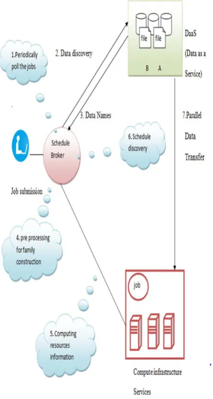
DaaS (data as a service ), the idea behind DaaS is to avoid the complexity and cost of running your own database. Let us assume there is one user sending the jobs/requests to scheduler broker. Scheduler broker regularly collects the jobs from the pool. Scheduler broker will divide two parts one with (DaaS) data as a service and another one is compute infrastructure service. Scheduler broker sends discovery data to DaaS (data as a service) and then it sends back data names to scheduler broker as pre processing for family construction based on data requirements. Scheduler broker it access the computing resource information to compute infrastructure services. The scheduler broker discovers the schedule from schedule discovery. finally, (DaaS) data as a service sends parallel data transfer to compute infrastructure services.
Fig 1. System Architecture
The workflow is depicted in Figure 2. The key activities in the workflow are: a) grouping the job based on the common/extended data which we call as the family construction, b) determining the data workloads between compute and simulated sites, and c) discovering the best schedule to minimize the turnaround time of the jobs. These activities are explained below.
Fig 2. System Workflow
A. Family construction
improvement and administration single and multi- region swift clusters.
Amazon S3[18] offers object keys and associated meta data tagged with the files/objects. Amazon was one of the first companies to offer cloud services to the public .Amazon offers a number of cloud services including EC2 (Elastic Compute Cloud ), S3 (Simple Storage Service), Simple Queue Service, Simple DB. Elastic compute cloud offers virtual machines and extra CPU cycles for your organization. Simple storage service allows you to store items up to 5GB in size in Amazon’s virtual storage service. Simple queue service allows your machines to talk to each other using this message passing API. Simple database is a web service for running queries on structured data in real time. Object meta data is are two ways : one with user defined meta data, user defined meta data tagged the extra information, and the second with system meta data, system defined meta data describes storage class information, object creation dates. First, we apply the query to discover the jobs with similar object identifier tags, followed by key/value pair combination for finding the common /overlap data.
B. Determining data workloads
The above figure(2) represents family job construction will be divided into two parts: one with determine the data hosts, and the second with determine the compute nodes. The data workload is determined based on the available bandwidth between replicated sites and the compute nodes. Available bandwidth is less the data workload is high, and the available bandwidth is high the data workload is less. Network traces between the computing resources and data hosts are used to estimate the channel bandwidth availability. Network traces based on RTT (Round Trip Time) over a time period is used as factor in our model to approximate the amount of data to be transferred from each of the simulated sites.
C. Optimal Schedule
Scheduling is a process of allocating jobs on to available resources in time, such process has to respect constraints given by the jobs and the cloud. Optimal schedule means best schedule, the schedule is based on steady state genetic approach using turnaround time minimization as fitness value. Steady state selection is not a particular method of selecting parents, main idea is this selection process is that big part of chromosomes should carry onto next generation. Each and every generation are selected good/bad results, in every generation selected few (good – with high fitness value) chromosomes for creating a new
offspring.
Then some (bad – with low fitnessvalue) chromosomes are removed and the new offspring is placed in their place. The rest of population carry on to new generation. Genetic approach using turnaround time minimization as fitnessvalue.
D. Data and applications migration
Based on the compute the group scheduling map with the data consolidation, data and application services would be moving one place to another place to the compute node and compute times for the family jobs.
E. Execution
Based on performance jobs completion on the compute nodes, and removal of the temporary and moving one place to another the data sets from the computing nodes.
F. Result
Result sent to the end user.
IV. METHODOLOGY
Here, we discuss the methodology concept for family construction.
A.Family construction
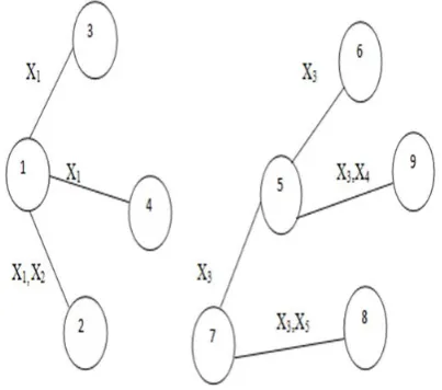
Here, we using graph data structure, we call here family graph is used for grouping the jobs. In this family graph there are nine jobs, job is represented as node and data required by both the jobs is represented by the edge. A sample family graph with 9 jobs numbered from 1 to 9, and four data sets named from X1 to X5 are shown in figure3.
The graph indicates that the jobs 1,2,3 and 4 require the data with id X1, the jobs 1 and 2 require the data with id X2, and jobs 5,6,7,8 and 9 require the data with id X3, the jobs 5 and 9 require the data with id X4, and jobs 7 and 8 require the data with id X5 for processing. The families are grouped by computing the connected components of the graph. The graph in figure 3, results in two connected components with the nodes 1,2,3 and 4 for th first component, the nodes with 5,6,7,8 and 9 for the second component. The resultant connected components form two family jobs or two groups. B. Notations used
Mathematical notations for the problem formulation are described in Table 1.
J = Total number of jobs
N= Total number of computing nodes in the grid. H= Total number of data service/providers F= Total number of families
Wf = Total number of jobs in the family f.
TDfi=Data Make Span(Consolidation time) in minutes of the family fϵF on Node i.
rhi = Estimated packet transmission time in seconds between data provider hϵH to compute node iϵN. Xf = Amount of data required in GB for the family fϵF.
Xfhi= Data chunk in GB from the data provider hϵH
to compute node iϵN for the family fϵF.
ρhi= Weight assignment to the channel from data provider hϵH to compute node iϵN.
TRJi= Turnaround time of the job j on node i. TSji= Setup time of the job j on node i. TAj= Arrival Time of the job j. Δfi= Decision variable.
δ
fi=
Assignment variable.
Table 1.Mathematical Notations
C. Objective Function
The objective is to minimize the turnaround time of the jobs over the computing nodes.
Minimize ∑Jj=1∑Ni=1∑F
f=1TRJIΔfiδfi
0 if j doesn’t belongs to f δf
j = 1 if j ϵ f
TRJI = TDFI/wf + TSJI + TLJI – TAJ
TRJI: Turnaround time of the job jЄf on computing node i.
TDfi: Data consolidation of the family f on computing node i.
TSji: Setup time of the job jЄf, on computing node i.
TLJI : Length of the job jϵf, on computing node i. TAj: Arrival /Submission time of the job jϵf. 1. Subject to the following constraints :
A family is assigned to either one compute node or none.
∑Ni=1Δfi ≤ 1 for f=1,2,……F Δfi ϵ {0,1}
Compute node can have either none or many families assigned to it.
∑F
f=1Δfi ≤ 1 for f=1,2,……N Δfi ϵ {0,1}
D. Determining the data consolidation time
Network traces between the computing resources and data hosts/providers are used to calculate approximately the channel bandwidth accessibility. The channel bandwidth availability is high the data workload is less, and the channel band width is low the data workload is more. Network traces based on the RTT (round Trip Time) over a time period is used as factor (weight factor) in our model to approximate amount data to be transferred from each of the simulated sites. Here, used a time period for estimate the amount of data to be transferred for the replicated sites, and to estimate the data quantity to moving from one place to another from each of data providers to compute node.
Graph data structure is constructed as family graph as considered in the fragment methodology of family construction. The family may have one are more jobs, and jobs depending on data requirements if they have common data. If each family consists of only one job, then F=J, otherwise F<J. Let wf be the number of jobs in the family f also called weight of the family, then w1+w2+…..+wF=J. In this scheduling the family job problems, data consolidation time is same for all the jobs that be in the right place to the same family.
Data Consolidation refers to the collection and combination of data from multiple sources into single destination. Data Consolidation time is defined as the maximum time to consolidate the data from the recognized data providers to the compute node. Data Consolidation time TDfi, is the maximum time necessary to bring the data from the data provider(s) to the compute node i for the family f, and is defined as
TDf i= maxh=1,H(Xfhi* rhi) (1) Where Xf
hi is the chunk size and rhi is the estimated time from the preceding historical traces, for the family f from data provider h to compute node i. Xf
hi can be computed as below. Xf
hi=ρhi*Xf (2)
Where Xf is total data size required for the family f, and ρhi denotes the weight assigned to the channel from host h to compute node i, is defined as ρhi = (1/ rhi)/∑Hi=1(1/ rli) (3) equation (3) is substitute by equation (2) Xf
hi =(1/ rhi)/∑Hi=1(1/ rli)*Xf (4) (4) After,substitution will get the equation (4)
Equation (4) is substitute by equation (1) TDfi=((1/rhi)/∑Hi=1(1/rli)*Xf*rhi) (5)
The time is estimated using the preceding history of packet transmissions over a time period. Simplifying equation (1), using equations (2) and (3) and (4), we get
TDf I = ((1/ rhi)/∑Hi=1(1/ rli) * Xf * rhi) = Xf / ∑Hi=1(1/ rli)
Family to node calculating is described as the heavy matrix. The problem can be solved as the bipartite assignment problem, but the restrictions are, a node can have maximum of one family designated, although it has sufficient processing
elements for handling more than one family. Hence, this problem reduces to 0/1 knapsack which can be solved using greedy, dynamic programming or evolutionary techniques like genetic algorithms. In the proposed group scheduling, three probable schedules may take place for the computing nodes during execution, such as:
(i) No family assigned.
(ii) With exactly one family assigned. (iii) More than one family assigned.
Based on the schedules illustrated as above for a compute node, we consider below the GA problem formulation, chromosome representation, scheduling algorithm and the results obtained with the duplicated data.
GA PROBLEM FORMULATION
Steady State Genetic Algorithm [7] is used by replacing percentage of chromosomes across the generations until the solution meeting or till the maximum number of generation is reached. Genetic algorithm library (GALib) [19] is used for implementation.
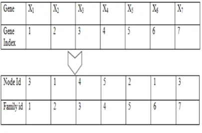
A . Chromosome representation
We select integer based data formation for genomes representation. The gene index represents the familyid, and the genomes demonstrate the compute nodeid to which the family is mapped. The data formation of the chromosome is shown Figure 4.
Figure 4.Sample chromosome
familyid=2 is assigned to nodeid=1, and so on. From the above figure it is also seen that nodeid=3 has been assigned with familyid=1 and 7; nodeid=1 has been assigned with familyid=2 and 6; nodeid=4 has been assigned with familyid=3; nodeid=5 has been assigned with familyid=4; nodeid=2 has been assigned with familyid=5 and nodeid=6,7, and 8 have not been assigned to any family.
B. Evolve method
An early population of chromosomes are preferred at random and the fitness function is applied. The fittest chromosomes are carried to the next generation based on the Steady State extend beyond percentage of chromosomes. The process is reproduced either till the maximum elementary runs are finished or the meeting of the objective value is achieved. In order to select the fittest chromosomes for the next generation the operators like crossover and mutations are used. The next generation chromosomes are produced by genetically mating fitter individuals of the current generation.
C. Scheduling algorithm
Table 2 describes the fitness function pseudo code and Table 3 discusses the proposed GA for scheduling the family jobs using the fitness function.
Table 2:Fitness Function Pseudo code
Algorithm: Fitness function F pseudo code Input: Chromosome C
Output: Turnaround time of the schedule
1 Turnaround time T:= 0
2 For all genes in the Chromosome C perform the following steps do
3 read gene index f and genome value i 4 Compute the jobs {J}ϵ to f.
5 For all jϵJ do
6 Estimate data consolidation time TDfI , compute total jobs wf in family f.
7 Compute setup time TSfI , estimated job length on node i, TLJI and arrival time TAJ. .
8 Compute the turnaround time TRJI of job jϵJ on computing node i.
9 TRJI = TDfI/wf + TSJI + TLJI – TAJ 10 T := T + TRJI
11 end for
12 until end of chromosome
13 return T;
Table 3 GA for schedule discovery
Algorithm: Scheduling Algorithm pseudo code Input: Population, Generations, Crossover percent,
Mutation percent, Gene length, Percentage of chromosome to carry forward (P. g, c, m, l, r)
Output: A Schedule for all the jobs
1. Initial Run: Randomly generate population P chromosomes.
2. Repeat
3. Calculate the fitness of all chromosomes using
Fitness function F
4. Arrange the population in the ascending order of fitness value
5. Copy the r best chromosomes to new population. 6. for the remaining chromosomes; perform the crossover with percent c and mutationWith percent m. Copy the new off springs to new population. 7. Replace the current population with the new population
8. Until maximum generations or convergence.
V. EXPERIMENTS AND RESULTS
locations that provide 40 data storage nodes with interrelated imitated bandwidths
.
The following experiments are conducted in the order described below
.
A. Data consolidation Analysis Observations are conducted to learn the data transfer and consolidation timings from single site vs. the multiple duplicated data sites allowing for the network traces over a time period. B. Determining optimal probabilistic values of
genetic operators
Observations are organized to derive the best values of Genetic Algorithm (GA) operators for cross over, mutation and types of crossovers
.
C. Comparing with match making and heuristic techniques
The algorithm is related with match making techniques like Data First, Compute First, and heuristics such as Simulated Annealing (SA).
D. Comparison with Non family scheduling The algorithm is correlated with Non family i.e. without grouping the jobs.
Resource
name Type Virtual elements/bandwidths processing CHYD1-7 Virtual
Compute provider
200/100Mbps-200 Mbps#
CBGL1-6 -do- 500/50Mbps-100Mbps CMUB1-7 -do-
400/100Mbps-500Mbps CDEL1-8 -do-
300/20Mbps-200Mbps HYDS1-5 Virtual
data provider
0/100Mbps to 200Mbps## BGLS1-10 -do- 0/10Mbps to
100Mbps
MBS1-10 -do- 0/256 to 512 Mbps RJPS1-15 -do- 0/56 to 128 Mbps
Table 4.Simulated configuration of Big data clouds
1-7 indicates a total of 7numbers.
#200/100Mbps to 200Mbps specify randomly generated PEs with a maximum of 200 for each compute supplier, with the network channel bandwidth randomly simulated between 100 Mbps to 200Mbps.
##0/100 Mbps to 200Mbps represents the randomly generated data source without computing elements, the bandwidth varying from 100 to 200 Mbps for a sum of five data providers.
The experiment are replicated for a total of 1000 jobs with 40 virtual data providers and the network traces generated randomly between the virtual computing nodes and data providers. Based on the network traces average packet transmission times is expected over a time period from data supplier to computing nodes.
A. Data consolidation analysis
Graph 1depicts the data consolidation times when the exacting data storage and several simulated storage repositories are used. The conclusion indicates that, data relocation time from simulated sites is improved than from a single site.
Graph1. Data transfer times in replicated vs. Single
B. Determine the probability value for genetic operators
The experiments are conducted to determine the genetic operators and the possibility values needed for the GA operators, for an upper limit of 1000 jobs over a program phase is discussed. a number of experiments are organized to determine the crossover operator among one point, two point, uniform, and roulette wheel. The experiments are performed by fixing the cross over and mutation operators to 0.9 and 0.01 and unbalanced the population length and generations to study the meeting of the fitness value. The conducted experiments are shown in Table 5, the resultant fitness values from the experiments are depicted in Graph 2.
Table 5.Experiments to determine genetic operators
Exp .no Pop Length Total no.of generations
1 50 50
2,3 100 200
4,5,6 200 100
7,8,9 300 200
10,11,12 300 300
0 50 100 150 200
1 3 5 7 9 11 13 15
Time(sim.units)
Job id
Consolidation
time from
replicated sites
Consolidation
time from a
The experiments indicates in Graph 2 determine the roulette wheel has improved convergence across the generations while compared to the other genetic operators. Hence, the roulette wheel operator is chosen for cross over operations for the subsequently level experiments.
Graph 2. Fitness value comparison for genetic operators
In the next step, the experiments are
conducted for determining the cross over
and mutation probabilities while fixing the
roulette wheel cross over operator. The
experiments are conducted for 200
generations, with an
initial cross over
probability value of 0.5, up to 0.9, with
an
increasing value of 0.1 in each step. The
consequent fitness values obtained are
illustrated in
Graph 3. The results point to
roulette wheel cross over operator with the
probability value of 0.9 has better
convergence over the other examine
probability values.
Graph 3. Fitness value convergence across generations
Experiments are performed with varying mutation probabilities to determine the appropriate mutation ratio by fixing cross over operator of 0.9 and roulette wheel, the experiments shown in Graph 4 indicates with mutation probability of 0.01 has the better meeting fitness value.
Graph 4. Mutation probability
C. Comparing with other techniques
The proposed GA is correlated with match making and heuristic techniques discussed below. Here, two types of match making techniques such as Minimum Data consolidation First and Minimum Compute First are used. soon after, heuristic technique such as Simulated Annealing techniques is discussed. The retrieve results are compared with theproposed GA move toward which is depicted in Graph 5.
Graph 5. Comparing GA with other techniques 0
100 200 300 400 500 600 700 800 900 1000
1 2 3 4 5 6 7 8 9 10 11
Fitness
value
single point
Two point
uniform
Roulette
Experiment No
0 200 400 600 800 1000 1200
1 2 3 4 5 6 7 8 9
Fitness
value
0.9
0.8
0.7
0.6
0.5
Generation .No
0 2000 4000 6000 8000 10000 12000
1 2 3 4 5 6 7 8 9 10
Fitness
value
0.001
0.005
0.01
0.015
0.5
Genration .No
0 200 400 600 800 1000 1200
1 2 3 4 5 6 7 8 9 10
Makespan
(Sim.Units)
GA
SA
MinData First
1.Minimum Data consolidation First at node:
In
this mapping, a calculate resource that
ensures minimum data consolidation time
is selected for the family.
2.Minimum Compute First:
In this mapping, a
compute resource that ensures the
minimum calculation time is selected for
the family.
3.Simulated Annealing:
In this mapping
heuristics are applied by removal the worst
fit values from the present state to the next
state and moving towards the best
collection. The results indicate that
Minimum Compute First technique has
resulted in larger makespan while
correlated to Minimum Data First and SA
techniques. Minimum Data First and
Simulated Annealing techniques have
almost the similar makespan value with
performance better than Minimum
Computer Fist technique. However, the
proposed GA has resulted in minimal
makespan while correlated to
matchmaking techniques and SA. This
might be due to the normal evolution
actions of GA and fitness functions used to
get the near best solution.
D. Performance comparison of family vs. non family scheduling
Experiments are conducted for analyzing
the turnaround times for the families and
non-families from a single repository vs.
imitation repository. The results depicted
in Graph 6, represent that turnaround time
is less from the replicated sites while
compared to the results from the single
site, which is due to the minimal data
consolidations from replicated sites.
Another set of experiments are performed
for analyzing the turnaround times of
family vs. non family scheduling. This is
carried out by applying the data
relocation/consolidation from the
simulated sites to the preferred computing
nodes.
Graph 6. Turnaround times of non family
Graph 7 represents, the jobs with the family
grouping has resulted in minimal turnaround time while compared to the non-family. This is due to the data consolidation carried out one time for the entire family job. This would reduce the data migration overheads for each job and reduce the network bandwidth consumptions. However, for few jobs the resultant turnaround time is more while compared to non-family scheduling
.
Graph 7. Turnaround Times for Family Vs. Non Family
The longer data consolidations is due to more numbers of jobs in the family, and the longer computing times is due to the accessibility of minimal computing essentials at the selected compute node than actually demanded for processing.
VI. CONCLUSION AND FUTURE WORK
The proposed family/group scheduling model addresses the data demanding problems to minimize the turnaround time of the jobs where the computing and data resources are decoupled. The jobs with familiar data are grouped together, based on the family graph and linked components to
0 1000 2000 3000 4000 5000 6000
1 2 3 4 5 6 7 8 9 10
Turnaroundtim
e
(Sim.Units) Singleprovi
der
replic ated sites
Jobid
0 5 10 15 20 25 30 35 40
1 2 3 4 5 6 7 8 9 10
Turnaround
time(sec) Non
Family
Family
which a similar data approach is applied. Steady state GA is applied to determine the best schedule.
The results are illustrated for the both family and non-family schedules from a single site and multiple replicated sites. The results shows that, data relocation from replicated sites illustrate performance improvement over a single site. The experiments also show that family schedule performs improved over the non-family schedule, whenever the grouped jobs do not beat the obtainable node capability
In future, it is proposed to use Rough Set theory for the grouping. The algorithm is tested with time shared scheduling plan. In prospect the studies would be conducted on space mechanisms such as buddy system, DHC (Distributed Hierarchical Control), Ouster out matrix, and bin packing. The algorithm would be customized to map the family job to the node where data is previously present, which would remove the data consolidation time.
The structure throughput is decreased while the family capacity exceeds the obtainable node capacities. Hence, a study is requisite to schedule such families, by adding a price to the total calculates time, so that the improved node could be selected for scheduling. This paper addresses the relocation of the data based on network traces over a time period; however, a detailed study is required to prepare the system for dissimilar network traffic conditions.
The proposed algorithm can be extended for limit and budget constraints. Currently, the model executes the jobs after the data is consolidated for the family; however, the studies can be conducted for the execution soon after the data for the job is made available.
REFERENCES
[1] Somasekhar G, Karthikeyan K. The pre big data matching redundancy avoidance algorithm with mapreduce. Indian Journal of Science and Technology. 2015 Dec; 8(33). DOI: 10.17485/ijst/2015/v8i33/77477.
[2] Lakshmi M, Sowmya K. Sensitivity analysis for safe grainstorage using big data. Indian Journal of Science and Technology. 2015 Apr; 8(S7). DOI: 10.17485/ijst/2015/v8iS7/71225.
[3 ] Liu J Liu F, Ansari N. Monitoring and analyzing big traffic data of a largescale cellular network with Hadoop. IEEE Network. 2014; 28(4):32–9.
[4] Mamlouk L, Segard O. Big data and intrusiveness: Marketing issues. Indian Journal of Science and Technology. 2015 Feb; 8(S4). DOI: 10.17485/ijst/2015/v8iS4/71219.
[5] Noh K-S. Plan for vitalisation of application of big data for e-learning in South Korea. Indian Journal of Science and Technology. 2015 Mar; 8(S5).DOI:10. 17485/ijst/2015 v8iS5/62034.
[6] Z. Michalewicz: Genetic Algorithms + Data Structures=Evolution Programs. 1992, Springer.
[7] Goldberg D.E., Genetic Algorithms in search, Optimization and Machine Learning, Addison Wesley , Reading ,MA,1989.
[8] K. Ranganathan, and I. Foster, “Decoupling Computation and Data Scheduling in Distributed Data-Intensive Applications”, Proc. 11th IEEE Symposium on High Performance Distributed Computing (HPDC). Edinburgh, UK, USA, July 2002.
[9] T. Phan, K. Ranganathan, and R.Sion, “Evolving toward the perfect schedule: Co scheduling job assignments and datareplication in wide-area systems using a genetic algorithm”, Proc. 11th Workshop on Job scheduling Strategies for Parallel Processing. Cambridge MA: Springer-Verlag, Berlin, Germany, June 2005.
[10] H. Mohamed, and D. Epema, “An evaluation of the closeto-files processor and data co-allocation policy in multiclusters”, in Proc. 2004 IEEE International Conference on Cluster Computing, San Diego, CA, USA, Sept. 2004.
[11] S. Venugopal, Scheduling Distributed Applications on Global Grids, Ph.D. Thesis, University of Melbourne, Australia, July 2006.
[12] Apache Hadoop, http://hadoop.apache.org/ (15.06.2014).
[13] Fair Scheduler ,
http://hadoop.apache.org/docs/r1.2.1/fair_scheduler.pdf(11 .06.2014)
[14] Capacity Scheduler, http://hadoop.apache.org/docs/r1.2.1/capacity_scheduler.p df (11.06.2014)
[15] S. Gupta, C. Fritz, R. Price, J. D. Kleer, and C. Witteveen, Throughput Scheduler: learning to schedule on heterogeneous Hadoop clusters, Proceedings of the International Conference on Autonomic Computing, ICAC 2013, June, 2013, San Jose, CA, USA.
[16] L. Shi, X. Li , and K.L. Tan, S3: An efficient Shared Scan Scheduler On MapReduce Framework, International Conference on Parallel Processing, ICPP 2011, Taipei, Taiwan, September 2011.
[17] OpenStack Swift, Object Based Storage and REST Services, http://swiftstack.com/openstack-swift (5.3.2014). [18]AmazonS3: www.aws.amazon.com/s3(2.2.2014).
[19] Java GA Lib, Genetic Algorithm Library: http://sourceforge.net/projects/java-galib (11.06.2014).