Characterization Method of an Automotive Random-LOS OTA
Measurement Setup
Aidin Razavi1, *, Andr´es Alay´on Glazunov2, 3, Sadegh Mansouri Moghaddam3, Rob Maaskant3, 4, and Jian Yang3
Abstract—A novel characterization method of OTA test setups for wireless communication systems on vehicles in the random line-of-sight (Random-LOS) environment is proposed. The measurement setup assumes a compact range and a test zone where the antenna under test (AUT) on the vehicle would be located. An ideal receiver is assumed for the reference measurement, which allows to perform a system analysis through evaluating the Probability of Detection (PoD) as the system figure-of-merit. The proposed method is aimed as an aid for test equipment designers to design OTA compact ranges, compare their performances, and define an ideal numerical reference. The requirements for OTA measurement ranges are different from those for conventional anechoic compact ranges. A compact cylindrical reflector system with an antenna array line feed is characterized using the proposed method, from 1.6–2.7 GHz, for two orthogonal polarizations, various AUT heights and reflector tilting angles, with and without ground plane in a test zone which is 2 m wide in diameter.
1. INTRODUCTION
The automotive industry is in urgent need to meet the ever increasing consumer connectivity demands for, e.g., easy access to online maps and satellite navigation systems, infotainment systems and music and video streaming services. Higher number of wireless links to and from vehicles are expected, delivering satisfactory quality of service and ensuring passenger safety. Therefore, next generation over-the-air (OTA) measurement systems are required to evaluate the end-to-end performance of the wireless communication links to and from vehicles [1], whose numerical characterization is the subject of the present paper.
In system level OTA tests, parameters such as antenna radiation pattern or directivity are usually of no interest. Instead, OTA testing of wireless systems is performed in an emulated propagation environment with the objective to evaluate the system performance in a repeatable and controllable way. It can be performed in both anechoic chambers (with absorbing walls) and reverberation chambers (with reflecting walls and mode stirrers) [2, 3]. In traditional antenna measurements, anechoic chambers are used to emulate the free space channel [4]. We call it pure Line-Of-Sight (LOS) propagation channel, since it is useful to characterize fixed antenna installations with little or, in the limiting case, no fading at all. On the other hand, the reverberation chamber is useful to emulate the Rich Isotropic MultiPath (RIMP) propagation channel, i.e., the other limiting case [5, 6]. RIMP emulates the propagation channels encountered in urban or indoor environments where scattering is the main contributing propagation mechanism leading to severe fading of the received signal [2]. Furthermore,
Received 2 April 2018, Accepted 28 April 2018, Scheduled 14 May 2018 * Corresponding author: Aidin Razavi ([email protected]).
anechoic chambers have become popular in OTA measurements using multiprobe antenna systems to generate various channel models [7–12].
For automotive wireless communication links, especially in areas where the density of scatterers is low, e.g., highways and rural areas, the LOS channel component is expected to dominate over the RIMP propagation channel component. This effect increases with frequency [13]. The same is true in mm-wave 5G wireless systems where the combination of smaller cells, beam forming, and higher penetration losses leads to LOS being more pronounced than multipath. However, due to the random orientation of a vehicle relative to base stations, the fixed LOS assumption is no longer applicable to such communication links. Instead, the Random-LOS propagation scenario becomes more suitable to describe this new OTA test scenario, where the propagation channel exhibits slow fading rather than fast fading variations [14, 15]. More sophisticated channels that take into account signal blockage, e.g., by other vehicles can be incorporated by means of channel emulators, when such models become available. In conventional antenna measurement setups it is often desired to realize an incident plane wave in the immediate vicinity of the device under test. In these scenarios the radiation pattern is often required with an accuracy of a tenth of dB or less, and the test setup’s figure of merit is typically the ratio between the energy in the error field and the ideal plane wave [16, 17]. The plane wave can be synthesized by a number of different methods, e.g., using a reflector in a compact range [18], determining a continuous aperture current source by iterative methods and then discretizing the current distribution for a number of probes [19, 20] or direct calculation of the excitation weights for regular [21, 22] and sparse [23] arrays.
In OTA measurements of the performance of wireless communication systems, a statistical approach is chosen which involves many measurements of an entire communication system inside the testing zone. These measurements are often based on certain probability levels (e.g., 90% or 95%) of PoD of bit streams or CDFs of measured signals, or communication throughput curves. Synthesized plane waves have also been studied before in the context of OTA measurements of MIMO antennas in multi-probe [9, 10] or compact range setups [24, 25]. While the uniformity of the field can also be described by the CDF of radiated power, it is not strictly required for OTA test chambers. In fact, in OTA testing, a proper characterization of the field distribution in the reference test zone is more important than its uniformity. In other words, generation of a plane wave is desired, but since OTA testing involves, e.g., throughput measurement, it is sufficient to have a good enough field uniformity. As a result, the design requirements are also different, i.e., the uniformity of the quiet zone can be substantially relaxed resulting in less complex and thus cheaper test chambers. For example, reflector edge treatment can be avoided.
Test zone characterization of multi-probe setups in anechoic chambers for MIMO OTA measurements based on parameters such as MIMO throughput [11] and channel capacity [12] has been tried before. In the present paper we propose a new method for test zone characterization of OTA measurement setups for the Random-LOS environment. In the proposed method we employ the ideal threshold receiver model [26] and PoD functions to define a new figure of merit based on the performance of a communications system as a whole.
The novelty of the present work therefore involves: (i) the proposal of a realistic and advantageous compact test range for active OTA characterization of wireless devices whose antennas are mounted on the body of a car; (ii) a numerically fast characterization method that is based on a system performance figure-of-merit (FoM) rather than only on the antenna impedance and radiation characteristics; (iii) a new system FoM which is based on the statistics of the PoD of a transmitted data bitstream [26]. The impact of the direct feed radiation on the total field and PoD characteristics are examined as well. It must be noted that the reflector and the bowtie array feed in the presented results are optimized for 1.6–2.7 GHz frequency range. This does not mean that the proposed characterization method is inherently limited to this frequency range. The proposed method and metrics can invariably be applied to other frequency bands such as mm-Wave frequencies, in order to design test setups suitable for such frequencies.
hr
Lr
Feed array
h
Cylindrical
Test zone
R
D F
reflector
L
AUT
f
θ x
y z
(a) (b)
Figure 1. (a) Artist impression of a compact OTA measurement setup: A chamber antenna, vehicle under test, turn table. (b) The numerically considered system: Array-fed cylindrical reflector, ideal receiving probe antenna (AUT) at a random location within the test zoneS.
before, are now taken into account [27]. Furthermore, more realistic bowtie antenna elements (optimized for 1.6–2.7 GHz) are assumed for the array feed [28, 29], as opposed to those assumed in [27, 30]. The measurement setup is therefore smaller in size, of lighter weight and thus easier to tilt than conventional compact ranges [18]. Other alternative automotive OTA measurement techniques employing anechoic chambers propose the use of multiprobe antenna systems [31], but will not be considered in the present characterization study.
The studied measurement setup is described in Section 2, the characterization method in Section 3, followed by the results and conclusions in Sections 4 and 5, respectively.
2. RANDOM-LOS OTA MEASUREMENT SETUP
The vehicle under test in Fig. 1(a) is located on a rotating platform and a communication tester (not shown) is connected to the array-fed reflector, i.e., thechamber antenna. The vehicle rotation emulates the random azimuthal angle-of-arrival (AoA) of the incoming LOS wave from the base station. The transmitted signal is vertically or horizontally polarized, or it can be dual-polarized. Depending on the distance between the AUT and the axis of rotation during the test, the AUT will move in a circular path. Since the exact radius of this path can vary, we refer to a circular area of radiusRas thereference test zone S and study the statistics over the whole area ofS instead of the circumference of a specific circle. The dimensions of the test zone depend on the antenna location on the vehicle as well as the vehicle size. If the antenna is located on the vehicle’s roof, the radius of S can be up to 1 m for typical personal vehicles. Different elevation AoAs due to different base station heights are emulated by tilting the chamber antenna.
As explained in the Introduction, the degree of field homogeneity inside the test zone is not the primary system FoM for the considered OTA measurement setup, as this would result in too stringent design requirements. However, the field homogeneity is inherent in the PoD when the location of the receiver probe inside the test zone is random.
3. TEST ZONE CHARACTERIZATION
3.1. Ideal Threshold Receiver Model and PoD
The IDTR model is based on the fact that in modern communication systems which employ advanced error correction schemes, the error rate will abruptly change from 100% to 0% in a stationary Additive White Gaussian Noise (AWGN) channel as soon as the received signal-to-noise-ratio (SNR) exceeds a certain threshold [26].
According to the IDTR, when the received signal undergoes fading, the relative system throughput can be represented by
TPUT(P/Pth)
TPUTmax
=PoD(P/Pth) = 1−CDF(Pth/P) (1)
where Pth is the threshold level of the receiver, P a reference value proportional to the transmitted
power, PoD the Probability of Detection function, CDF the Cumulative Distribution Function (CDF) of the received power at the input of the threshold receiver normalized to P, and TPUT the system throughput. The reference value P is usually chosen as either the average of received power or the maximum received power. However, the exact choice of P does not affect the model and any value proportional to the transmitted power can be chosen. The CDF is taken over the test zone when the transmitted power is constant. The fraction P/Prmth is given in dBt, i.e., the dB value relative to the receiver threshold level. In the current Random-LOS setupP is chosen as the average received power over the entire test zone†. The dBt value at a certain PoD level can be used as an indicator of the system performance: a larger dBt value means higher transmitted power is required to maintain the same PoD level, resulting in a poorer system performance. Thus, the dBt value at high PoD levels is desired to be as small as possible.
3.2. Figures of Merit
If the received power is perfectly homogeneous over the test zone, then the CDF and consequently the PoD will be an ideal vertical line at 0 dBt. Hence, the deviation of the PoD function in Eq. (1) from the ideal vertical line can be used as a measure of the variation of the radiated field in the test zone. We will define the system throughput-based FoM as the dBt value at the 90% PoD level:
P0.9=PoD−1(0.9), (2)
wherePoD−1 is the inverse function ofPoD as defined in Eq. (1).
In an ideal measurement setup, the direct radiation from the feed in the test zone (S) must be negligible, i.e., Ei(r∈S) =0, which means that Et =Ei+Es =Es forr∈S, where ris the location
vector of the points in the test chamber. Furthermore,Ei,Es,Et are the direct radiated field from the feed, the scattered field from the reflector, and the total electric field in the test zone. In addition, if the scattered fieldEsrepresents locally a plane wave, then we haveP0.9= 0 dBt. In practice, the feed is
designed to optimally illuminate the reflector, hence, |Es|2 |Ei|2 for r∈S. Accordingly, P0.9 ≈Ps0.9,
wherePs0.9 is computed using (2) when the scattered field substitutes the total field.
To quantify the contribution of Es to variations in Et, it is instructive to compute and examine the parameter
ηs=|Ps
0.9−P0.9| (3)
which measures the contribution to the variation in the total field — also indirectly via the system PoD — due to the far-side and back-lobe radiation of the array feed. Clearly, ηs = 0 if no such detrimental effects exist.
4. NUMERICAL RESULTS
The simulations were carried out in MATLABR 2013b on a Windows 7 PC — Xeon E5-2640 @2.5 GHz, 256 GB RAM.
planar array chamber antenna for the same application and requirements [30], we choose F = 1.5 m, hr = 3 m and Lr = 4 m. The height of the test zone (h) depends on the height of the vehicle under
test and can vary between 1.5 m and 2 m. The main beam of the focal line array feed of dual-polarized bowtie elements (cf. [28] for element geometry) makes an angle θ with the negative direction of the z-axis. Based on previous models with Huygens sources as the feed [27], we have chosen θ= 55◦. The bowtie elements and the corresponding feed corrugations have been optimized for optimal illumination of the reflector. Both a hemispherically absorbing anechoic chamber with perfectly reflecting floor, and a spherically absorbing chamber are considered.
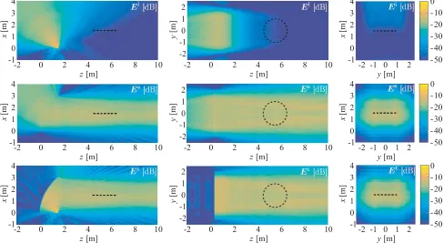
The embedded far-field radiation patterns of the bowtie elements are used to obtain the magnetic fieldHithat is incident on the reflector surface. The Physical Optics (PO) currentJ= 2ˆn×Hi is then computed in the center of each rectangular mesh cell and then multiplied by its cell area to arrive at its corresponding dipole moment. The mesh cell edge length isλ/2, which leads to only 1400 electrical dipoles at 1.5 GHz‡. The scattered field Es from the reflector in the test zone at 721×101 = 72821 points is then obtained by using the integral expressions in [32, Sec. 4.2]. The direct far-field radiation from the feed, Ei, is added to Es to yield the total fieldEt. The normalized intensity of Ei,Es, andEt @2 GHz are visualized in Fig. 2 (for vertical polarized field). The total average runtime for computations of one antenna setup over the frequency band (16 points) is∼50 min, of which only 25 sec is needed for the meshing and 110 sec for the PO current computations (no ground plane). The remainder is spent on the field computations in the test zone.
-2 0 2 4 6 8 10
-1 0 1 2 3 4 z[m] x [m]
-2 0 2 4 6 8 10
-2 -1 0 1 2 z[m] y [m]
-2 -1 0 1 2 -1 0 1 2 3 4 y[m] x [m] - 50 - 40 - 30 - 20 - 10 0
-2 0 2 4 6 8 10
-1 0 1 2 3 4 z[m] x [m]
-2 0 2 4 6 8 10
-2 -1 0 1 2 z[m] y [m]
-2 -1 0 1 2 -1 0 1 2 3 4 y[m] x [m ] - 50 - 40 - 30 - 20 - 10 0
-2 0 2 4 6 8 10
-1 0 1 2 3 4 z[m] x [m]
-2 0 2 4 6 8 10
-2 -1 0 1 2 z[m] y [m]
-2 -1 0 1 2 -1 0 1 2 3 4 y[m] x [m] - 50 - 40 - 30 - 20 - 10 0
Figure 2. The normalized intensity of the (top) incident, (middle) scattered and (bottom) total electric fields at 2 GHz in planar cuts parallel toxz,yzandxyplanes. The fields are normalized to the maximum of Et inxz-plane. The test zone is shown with the dashed line.
A 6 dB linear amplitude taper is applied to the three edge elements of the array at each end to reduce unwanted reflector edge diffraction effects. The induced current on the reflector surface, for the sample case of vertical polarization at 2 GHz, is shown in Fig. 3 for both tapered and not tapered feed arrays. The tapering clearly affects the currents around the edges of the reflector, thereby improving the FoMs significantly.
-2 -1 0 1 2 0 0.5 1 1.5 0
0.5 1 1.5 2 2.5 3
y[m] z[m]
x
[m]
-30 -20 -10 0
-2 -1 0 1 2 0 0.5 1 1.5 0
0.5 1 1.5 2 2.5 3
y[m] z[m]
x
[m]
-30 -20 -10 0
(a) (b)
Figure 3. The normalized amplitude of the induced surface current on the reflector for a 32 elements array at 2 GHz when (a) feed is excited with uniform amplitude, (b) linear amplitude taper is applied to the edge elements. The currents are normalized to the maximum of each case, in order to show the variations.
1.5 2 2.5 3
0 0.4 0.8 1.2 1.6 2 2.4 2.8
Frequency [GHz]
P0.9
[dBt]
24 elements 28 elements 32 elements
Ta pered No Ta per
1.5 2 2.5 3
0 0.4 0.8 1.2 1.6 2 2.4 2.8
Frequency [GHz]
P0.9
[dBt]
24 elements 28 elements 32 elements
Ta pered No Ta per
(a) (b)
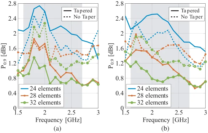
Figure 4. The power at 90% PoD level of the radiated field in the test zone vs. frequency, for different array length, both tapered and uniform amplitudes (a) horizontal polarization, and (b) vertical polarization.
We first examine the optimal length of the feed array (or number of elements), since the array element separation distance is already fixed at 11 cm (governed by the bowtie antenna geometry and grating lobe suppression requirements). Fig. 4 plots P0.9 for different array lengths vs. frequency,
antenna needs to be at least 3 m in order to have P0.9 below 1 dB [30]. This width corresponds to a
28-element line array for feeding the currently considered cylindrical reflector.
Based on the results in Fig. 4, a 32-element amplitude-tapered array is chosen as the feed for the chamber antenna.
4.1. Height Effects
Although the length of the feed array was determined for the height of the test zone h= 1.5 m relative to the feed, it is critical to be aware of the variations in the FoM due to changes in the elevation of the test zone.
The P0.9 for 1.5 m ≤ h ≤ 2 m, for both horizontal and vertical polarizations, is plotted in Fig. 5.
1.5 2 2.5 3
0.4 0.8 1.2 1.6 2
Frequency [GHz]
P0.9
[dBt]
h = 1.5 m
h = 1.6 m
h = 1.7 m
h = 1.8 m
h = 1.9 m
h = 2.0 m
1.5 2 2.5 3
0.4 0.8 1.2 1.6 2
Frequency [GHz]
P0.9
[dBt]
h = 1.5 m
h = 1.6 m
h = 1.7 m
h = 1.8 m
h = 1.9 m
h = 2.0 m
(a) (b)
Figure 5. The power at 90% PoD level of the radiated field in the test zone vs. frequency, for different heights of the test zone (h), with amplitude-tapered 32 elements array. (a) Horizontal polarization, and (b) vertical polarization.
1.5 2 2.5 3
0 0.1 0.2 0.3 0.4 0.5
Frequency [GHz]
η
s
h= 1.5 m h= 1.6 m h= 1.7 m h= 1.8 m h= 1.9 m h= 2.0 m
1.5 2 2.5 3
0 0.1 0.2 0.3 0.4 0.5
Frequency [GHz]
η
s
h= 1.5 m h= 1.6 m h= 1.7 m h= 1.8 m h= 1.9 m h= 2.0 m
(a) (b)
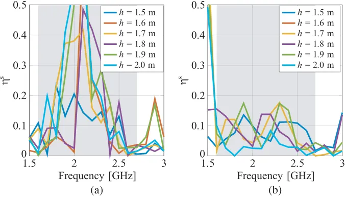
Note that the FoMs and their variations at higher elevations are close to those at h = 1.5 m, implying that similar level of measurement accuracy can be maintained for different vehicle heights. Unfortunately there is no straightforward relation between the elevation and the measurement accuracy level. The
P0.9 for vertical polarization is slightly less affected by the elevation at lower frequencies than for the
horizontal polarization. Higher accuracy in the vertical polarization is more essential than the horizontal polarization since most wireless communication links on vehicles are vertically polarized. The ηs for different h is plotted in Fig. 6 for both the horizontal and vertical polarizations. When ηs → 0, the field variation in S is governed by Es. Comparing this figure to Fig. 5 shows that in general low ηs corresponds to lower P0.9. In conclusion, the reference measurement is seen to be generally affected
by direct radiation from the feed in the test zone. Finally, a reflector whose vertical offset can be mechanically adjusted allows one to measure on taller cars as an alternative to using a fixed setup employing a larger reflector.
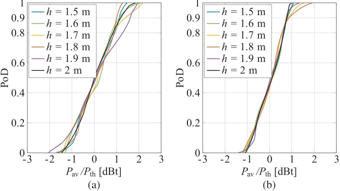
The impact of field variations on the PoD curves for different values of h at 2 GHz is further illustrated in Fig. 7; the ideal vertical line at 0 dBt indicates a homogeneous field distribution. As mentioned earlier, the reference power P is often selected as the average of the received power. Pav in
Fig. 7 refers to this choice of the reference power. As also observed in Fig. 5, the elevation impacts the field variations for the horizontal polarization more than for the vertical one.
-3 -2 -1 0 1 2 3
0 0.2 0.4 0.6 0.8 0.9 1
Pav/Pth[dBt]
Po
D
h = 1.5 m
h = 1.6 m
h = 1.7 m
h = 1.8 m
h = 1.9 m
h = 2 m
-3 -2 -1 0 1 2 3
0 0.2 0.4 0.6 0.8 0.9 1
Pav/Pth[dBt]
Po
D
h = 1.5 m
h = 1.6 m
h = 1.7 m
h = 1.8 m
h = 1.9 m
h = 2 m
(a) (b)
Figure 7. The PoD curves at 2 GHz for different heights of the test zone (h), with amplitude-tapered 32 elements array. (a) Horizontal polarization, and (b) vertical polarization.
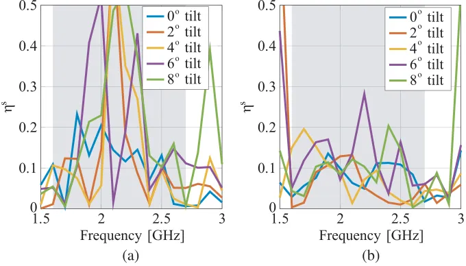
4.2. Tilting Effects
In practice, the base station antenna is usually at a higher elevation than the vehicle antenna, rendering the AoA of the incoming plane wave not parallel to the ground. This can be emulated by tilting the chamber antenna forward through including provisions in the mechanical design. In our model we will assume that the entire reflector-feed system rotates around its focal line, while the test zone remains in place.
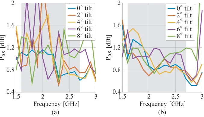
As expected, theP0.9 in Fig. 8 shows that an increase in tilt angle increases the uncertainty of the
measurement. Up to 8◦ the P0.9 is however mostly below 1.5 dB in 1.6–2.7 GHz band. Similar to the
elevation case, direct radiation from the feed exacerbates the field variations in the test zone. It can be observed in Fig. 9 that lower P0.9 values, correspond to lowηs values. The PoD curves for different
values of tilt at 2 GHz andh= 1.5 m are plotted in Fig. 10, which shows that highP0.9 corresponds to
1.5 2 2.5 3 0.4
0.8 1.2 1.6 2
Frequency [GHz]
P0.9
[dBt]
0 tilt 2 tilt 4 tilt 6 tilt 8 tilt
1.5 2 2.5 3
0.4 0.8 1.2 1.6 2
Frequency [GHz]
P0.9
[dBt]
0 tilt 2 tilt 4 tilt 6 tilt 8 tilt o
o
o
o
o
o
o
o
o
o
(a) (b)
Figure 8. The power at 90% PoD level of the radiated field in the test zone vs. frequency, for different values of mechanical tilt. Amplitude-tapered 32 elements array. (a) Horizontal polarization, and (b) vertical polarization.
1.5 2 2.5 3
0 0.1 0.2 0.3 0.4 0.5
Frequency [GHz]
η
s
0 tilt 2 tilt 4 tilt 6 tilt 8 tilt
1.5 2 2.5 3
0 0.1 0.2 0.3 0.4 0.5
Frequency [GHz]
η
s
0 tilt 2 tilt 4 tilt 6 tilt 8 tilt o
o
o
o
o
o
o
o
o
o
(a) (b)
Figure 9. ηs vs. frequency, for different values of mechanical tilt, with amplitude-tapered 32 elements array. (a) Horizontal polarization, and (b) vertical polarization.
4.3. Ground Plane Effects
-3 -2 -1 0 1 2 3 0
0.2 0.4 0.6 0.8 0.9 1
Pav/Pth[dBt]
Po
D
0 tilt 2 tilt 4 tilt 6 tilt 8 tilt
-3 -2 -1 0 1 2 3
0 0.2 0.4 0.6 0.8 0.9 1
Pav/Pth[dBt]
Po
D
0 tilt 2 tilt 4 tilt 6 tilt 8 tilt o
o
o
o
o
o
o
o
o
o
(a) (b)
Figure 10. The PoD curves at 2 GHz for different values of tilt at h = 1.5 m, with amplitude-tapered 32 elements array. (a) Horizontal polarization, and (b) vertical polarization.
test zone
ground plane 1
2 3
test zone
ground plane
1 2
3
(a) (b)
Figure 11. The diagram of the ray paths in the presence of ground plane when (a) no mechanical tilt is applied, and (b) mechanical tilt is applied.
1.5 2 2.5 3
0.4 0.8 1.2 1.6 2
Frequency [GHz]
P0.9
[dBt]
0 tilt 2 tilt 4 tilt 6 tilt 8 tilt
1.5 2 2.5 3
0.4 0.8 1.2 1.6 2
Frequency [GHz]
P0.9
[dBt]
0 tilt 2 tilt 4 tilt 6 tilt 8 tilt o
o
o
o
o
o
o
o
o
o
(a) (b)
Figure 12 plots P0.9 vs. frequency and shows that a tilt generally increases the reference
measurement uncertainty, particularly for the horizontal polarization, since the parallel component of Et to the ground plane is affected more than the vertical polarization (soft surface vs. hard surface,
resp. [33]). It is noteworthy that if a planar array (as in [30]) was used instead of the reflector, the higher
1.5 2 2.5 3
0 0.1 0.2 0.3 0.4 0.5 Frequency [GHz] η s 0 tilt 2 tilt 4 tilt 6 tilt 8 tilt
1.5 2 2.5 3
0 0.1 0.2 0.3 0.4 0.5 Frequency [GHz] η s 0 tilt 2 tilt 4 tilt 6 tilt 8 tilt o o o o o o o o o o (a) (b)
Figure 13. ηs vs. frequency, for different values of mechanical tilt, over infinite ground plane, with amplitude-tapered 32 elements array. (a) Horizontal polarization, and (b) vertical polarization.
- 2 0 2 4 6 8 10
-1 0 1 2 3 4 x [m]
- 2 0 2 4 6 8 10
-2 -1 0 1 2 z[m] y [m]
-2 -1 0 1 2 -1 0 1 2 3 4 y[m] x [m] -50 -40 -30 -20 -10 0
-2 0 2 4 6 8 10
-1 0 1 2 3 4 z[m] x [m]
-2 0 2 4 6 8 10
-2 -1 0 1 2 z[m] y [m]
-2 -1 0 1 2 -1 0 1 2 3 4 y[m] x [m] -50 -40 -30 -20 -10 0
-2 0 2 4 6 8 10
-1 0 1 2 3 4 z[m] x [m]
-2 0 2 4 6 8 10
-2 -1 0 1 2 z[m] y [m]
-2 -1 0 1 2 -1 0 1 2 3 4 y[m] x [m] -50 -40 -30 -20 -10 0
frequency grating lobes would be reflected from the ground plane and disturb the field distribution in the test zone. This effect is prevented by the current cylindrical reflector and bowtie array feed.
Theηs is plotted in Fig. 13 for different reflector tilts and polarizations. Again, the negative effect
of the direct feed radiation on the reference measurement accuracy is evident when this is compared with the trend of P0.9 in Fig. 12.
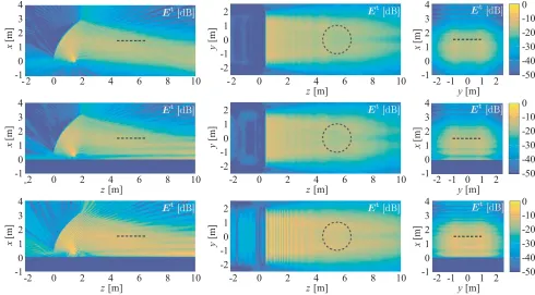
The total radiated field of the tilted chamber antenna in three planar cuts at 2 GHz is presented in Fig. 14, where the degradation effect of the ground plane on Et in S can be observed. It can be observed that the horizontal polarization is affected more than the vertical one, as described earlier.
5. CONCLUSION
We have proposed a characterization method for measurement setups intended for OTA measurements of the automotive wireless communication systems in Random-LOS environment. Along with the characterization method, a measurement setup consisting of a cylindrical reflector and a linear array feed of bowtie elements, in an anechoic or semi-anechoic chamber is introduced and characterized by the proposed FoMs, over the frequency band 1.6–2.7 GHz. It is shown that with proper choice of array length and amplitude taper, high accuracy can be achieved more easily than with a large planar array. The accuracy is assessed based on the PoD of an ideal receiver in a defined test zone. We have introduced a parameter to quantify the contribution of the scattered field to the variations of the field in the test zone, as opposed to that of the direct radiation from the feed. The direct feed radiation has a negative effect on the homogeneity of the field distribution in the test zone, thus also impacting the reference measurement accuracy. It is observed that the effect of the ground plane is more severe for the horizontal polarization, particularly when mechanical tilt is used to emulate elevated base stations. The presented characterization method will contribute to the design of OTA measurement setups that are smaller in size, of lighter weight and thus easier to tilt than conventional compact ranges. In the specific analyzed example of a reflector antenna systems, larger vehicles will be easier to accommodate and measure by only increasing the size of the reflector and the length of the array feed. The impact of the line array feed, as well as the reflector itself, on the field distribution within the test zone can be directly obtained by the outlined OTA characterization methodology.
REFERENCES
1. Kildal, P.-S., A. A. Glazunov, J. Carlsson, and A. Majidzadeh, “Cost-effective measurement setups for testing wireless communication to vehicles in reverberation chambers and anechoic chambers,”
2014 IEEE Conference on Antenna Measurements & Applications (CAMA), 1–4, IEEE, 2014. 2. De la Roche, G., A. Alay´on-Glazunov, and B. Allen, LTE-advanced and Next Generation Wireless
Networks: Channel Modelling and Propagation, John Wiley & Sons, 2012.
3. Kildal, P.-S., C. Orlenius, and J. Carlsson, “OTA testing in multipath of antennas and wireless devices with MIMO and OFDM,” Proceedings of the IEEE, Vol. 100, No. 7, 2145–2157, 2012. 4. Hemming, L. H., Electromagnetic Anechoic Chambers, Wiley Interscience, 2002.
5. Rosengren, K., P. S. Kildal, J. Carlsson, and O. Lunden, “A new method to measure radiation efficiency of terminal antennas,” 2000 IEEE-APS Conference on Antennas and Propagation for Wireless Communications, 5–8, 2000.
6. Arai, H., T. Urakawa, and M. Teranishi, “Radiation power measurement method of handheld terminals using compact shield box,” Electronics and Communications in Japan (Part I: Communications), Vol. 83, No. 8, 1984.
7. Fan, W., X. Carreno, P. Ky¨osti, J. Ø. Nielsen, and G. F. Pedersen, “Over-The-Air testing of MIMO capable terminals: Evaluation of multiple-antenna systems in realistic multipath propagation environments using an OTA method,”IEEE Vehicular Technology Magazine, Vol. 10, No. 2, 38–46, June 2015.
9. Laitinen, T., P. Ky¨osti, J.-P. Nuutinen, and P. Vainikainen, “On the number of OTA antenna elements for plane-wave synthesis in a MIMO-OTA test system involving a circular antenna array,”
Proceedings of the Fourth European Conference on Antennas and Propagation (EuCAP), 1–5, IEEE, 2010.
10. Wim, A. T., A. Heuberger, R. S. Thom¨a, et al., “On the accuracy of synthesised wave-fields in MIMO-OTA set-ups,” Proceedings of the 5th European Conference on Antennas and Propagation (EUCAP), 2560–2564, IEEE, 2011.
11. Fan, W., L. Hentil¨a, P. Ky¨osti, and G. F. Pedersen, “Test zone size characterization with measured MIMO throughput for simulated MPAC configurations in conductive setups,”IEEE Transactions on Vehicular Technology, 2017.
12. Toivanen, J. T., T. A. Laitinen, V.-M. Kolmonen, and P. Vainikainen, “Reproduction of arbitrary multipath environments in laboratory conditions,” IEEE Transactions on Instrumentation and Measurement, Vol. 60, No. 1, 275–281, 2011.
13. Rappaport, T. S., S. Sun, R. Mayzus, H. Zhao, Y. Azar, K. Wang, G. N. Wong, J. K. Schulz, M. Samimi, and F. Gutierrez, “Millimeter wave mobile communications for 5g cellular: It will work!,”IEEE Access, Vol. 1, 335–349, 2013.
14. Kildal, P. and J. Carlsson, “New approach to OTA testing: RIMP and pure-LOS reference environments & a hypothesis,” 2013 7th European Conference on Antennas and Propagation (EuCAP), 315–318, IEEE, 2013.
15. Kildal, P.-S., “Rethinking the wireless channel for OTA testing and network optimization by including user statistics: RIMP, pure-LOS, throughput and detection probability,”2013 Proceedings of the International Symposium on Antennas and Propagation (ISAP), Vols. 1 and 2, No. 1, 2013. 16. Hansen, J., Spherical Near-field Antenna Measurements, ser. Electromagnetics and Radar Series,
P. Peregrinus, 1988.
17. Hill, D., Theory of Near Field Phased Arrays for Electromagnetic Susceptibility Testing, ser. NBS Technical Note, National Bureau of Standards, 1984.
18. Johnson, R., H. Ecker, and R. Moore, “Compact range techniques and measurements,” IEEE Transactions on Antennas and Propagation, Vol. 17, No. 5, 568–576, Sep 1969.
19. Bennett, J. and E. Schoessow, “Antenna near-field/far-field transformation using a plane-wave synthesis technique,” Proceedings of the Institution of Electrical Engineers, Vol. 125, No. 3, 179– 184, IET, 1978.
20. Pereira, J., A. Anderson, and J. Bennett, “New procedure for near-field measurements without anechoic requirements,” IEE Proceedings of Microwaves, Optics and Antennas, Vol. 131, No. 6, 351–358, 1983.
21. Hill, D. A., “A circular array for plane-wave synthesis,” IEEE Transactions on Electromagnetic Compatibility, Vol. 30, No. 1, 3–8, 1988.
22. Haupt, R., “Generating a plane wave with a linear array of line sources,” IEEE Transactions on Antennas and Propagation, Vol. 51, No. 2, 273–278, 2003.
23. D’urso, M., G. Prisco, and M. Cicolani, “Synthesis of plane-wave generators via nonredundant sparse arrays,”IEEE Antennas and Wireless Propagation Letters, Vol. 8, 449–452, 2009.
24. Wang, H., J. Miao, J. Jiang, and R. Wang, “Plane-wave synthesis for compact antenna test range by feed scanning,” Progress In Electromagnetics Research M, Vol. 22, 245–258, 2012.
25. Parini, C., R. Dubrovka, and S. Gregson, “Optimizing a CATR quiet zone using an array feed,”
AMTA 2016 Proceedings, 1–6, IEEE, 2016.
26. Kildal, P.-S., A. Hussain, X. Chen, C. Orlenius, A. Sk˚arbratt, J. ˚Aberg, T. Svensson, and T. Eriksson, “Threshold receiver model for throughput of wireless devices with MIMO and frequency diversity measured in reverberation chamber,” Antennas and Wireless Propagation Letters, Vol. 10, 1201–1204, IEEE, 2011.
28. Moghaddam, S. M., P. S. Kildal, A. A. Glazunov, and J. Yang, “Designing a dual-polarized octave bandwidth bowtie antenna for a linear array,” 2016 10th European Conference on Antennas and Propagation (EuCAP), 1–4, April 2016.
29. Moghaddam, S. M., A. A. Glazunov, and J. Yang, “Wideband dual-polarized linear array antenna for random-LOS OTA measurement,”IEEE Transactions on Antennas and Propagation, March 9, 2018.
30. Alay´on Glazunov, A., A. Razavi, and P.-S. Kildal, “Simulations of a planar array arrangement for automotive random-LOS OTA testing,”10th European Conference on Antennas and Propagation, (EuCAP 2016), Davos, Switzerland, April 10–15, 2016.
31. Nilsson, M. G., P. Hallbj¨orner, N. Arab¨ack, B. Bergqvist, T. Abbas, and F. Tufvesson, “Measurement uncertainty, channel simulation, and disturbance characterization of an over-the-air multiprobe setup for cars at 5.9 GHz,” IEEE Transactions on Industrial Electronics, Vol. 62, No. 12, 7859–7869, Dec. 2015.
32. Kildal, P.-S.,Foundations of Antennas: A Unified Approach for Line-of-Sight and Multipath, Kildal Antenn AB, 2015, available at www.amazon.com and www.kildal.se.