Scholarship@Western
Scholarship@Western
Electronic Thesis and Dissertation Repository
6-22-2018 2:00 PM
Dynamics of the Phase Coupling for Flow, Heat and Mass
Dynamics of the Phase Coupling for Flow, Heat and Mass
Transfer in Conjugate Fluid/Porous Domains
Transfer in Conjugate Fluid/Porous Domains
Mahmoud Mohamed Mostafa ElhalwagyThe University of Western Ontario Supervisor
Straatman, Anthony G.
The University of Western Ontario
Graduate Program in Mechanical and Materials Engineering
A thesis submitted in partial fulfillment of the requirements for the degree in Doctor of Philosophy
© Mahmoud Mohamed Mostafa Elhalwagy 2018
Follow this and additional works at: https://ir.lib.uwo.ca/etd
Part of the Other Mechanical Engineering Commons
Recommended Citation Recommended Citation
Elhalwagy, Mahmoud Mohamed Mostafa, "Dynamics of the Phase Coupling for Flow, Heat and Mass Transfer in Conjugate Fluid/Porous Domains" (2018). Electronic Thesis and Dissertation Repository. 5437.
https://ir.lib.uwo.ca/etd/5437
This Dissertation/Thesis is brought to you for free and open access by Scholarship@Western. It has been accepted for inclusion in Electronic Thesis and Dissertation Repository by an authorized administrator of
ii
Abstract
Porous media prevail in industry e.g. heat transfer equipment, drying, food storage and
several other applications. Integrated in engineering, they form conjugate Fluid/Porous
domains. Physical modelling requires characterizing the microscale heat and mass
(moisture) transfer interstitially within porous media and their macroscale counterparts
across regional interfaces. Characterizing turbulence and its effects on phase coupling is
often needed too. The modeling literature survey shows phase coupling assumptions
depending on empiricism, phase equilibrium and lack of generality. Modeling of the
dynamic variations for the modes of phase exchanges, i.e. heat, mass and heat
accompanying mass exchanges, on both scales and generic turbulent coupling across
fluid/porous interfaces are absent. Thus, the objectives of this thesis are to, i) develop a
dynamic coupling model for phase heat and mass transfer in conjugate fluid/porous
domains, ii) validate the model in terms of interstitial phase exchange, macroscopic
interfaces and behaviors in different modes of heat and mass transfer, iii) extend the
model to turbulent flows characterizing turbulence correctly for different porosities and
permeabilities. The modeling process depends on a finite volume approach. Continuity,
momentum, turbulence, energy and mass equations are solved in point form for fluid
regions. In porous media, a volume averaged version is formulated and solved using one
equation per phase e.g. fluid temperature, solid temperature, vapor in fluid mass fraction
and liquid in liquid/solid mixture mass fraction. Mathematical conditions are utilised at
macroscopic interfaces reconciling the point-volume form differences, to ensure
continuity of conservation variables and numerical robustness. Physical phase exchange
formulae and numerical implementations for macroscopic interface heat/mass and
turbulence treatments are introduced. The model is validated interstitially by comparing
to experiments of Coal particles drying, for macroscopic coupling by comparing to
experiments and other models of apple and mineral plaster drying, respectively. The
results showed good agreement for all the cases. The turbulent coupling model has been
tested for a channel with porous obstruction high and low permeability cases and
iii
transfer was tested and produced physically correct trends and contours for apple and
potato slices drying.
Keywords
Dynamic Coupling, Heat and mass transfer, Computational Fluid Dynamics (CFD),
Porous media, Conjugate domains, Turbulence modelling, Low and high Permeability,
iv
Co-Authorship Statement
Chapter two is a published manuscript in international journal of heat and mass transfer.
The authors are, Elhalwagy, M. M. and Straatman, A.G.
Chapter three is a manuscript that will be submitted to a journal in the area of heat and
mass transfer. The authors are, Elhalwagy, M. M. and Straatman, A.G.
In both cases, the writing, research and analysis is carried out by myself, while the
v
Acknowledgments
I would like to thank GOD for providing me with the courage, patience and stamina to do
this work and for all his grants and blessings throughout my entire life.
I would like to express my gratitude and thanks to my supervisor, Prof. Anthony
Straatman. He is a true research leader and one of the best supervisors that a student can
have. His insight, guidance and continuous support have kept me going through this
journey and I always had him backing my steps and strengthening me.
I am grateful to my supervisory committee members, Prof. Eric Savory and Prof. Kamran
Siddiqui for multiple discussions and advice about my research topic. I am also grateful
to all my past and current colleagues in our CFD research labs for a great environment
and technical advice. This includes: Furqan Khan, Nolan Dyck, Shady Ali, Rajeev Kumar
and Ahmed Khalil. I also would like to thank Dr. Chris DeGroot for a lot of CFD
conversations. Thanks are also due to Professors Chao Zhang and M. Hesham Elnaggar,
as well as, the MME graduate coordinator Joanna Blom.
I would like also to take this opportunity to express my deep gratitude to my mother, May
she rests in peace, for all the support she gave me and for raising me and making me the
man I am now. I also had the care and support of my sisters and brother and for that I am
grateful. Special thanks are due to my wife Dina for being my companion through this
journey and standing by my side through the bad and the good times and, my children
Yusuf and Maryam for filling my life with love.
vii
Abstract ... ii
Co-Authorship Statement ... iv
Acknowledgments ... v
Table of Contents ... vii
List of Tables ... xi
List of Figures ... xii
List of Nomenclature ... xvi
Chapter 1 ... 1
1 Introduction ... 1
1.1 Background and scope to contribution ... 1
1.1.1 General Background ... 1
1.1.2 Scope ... 5
1.2 Literature survey ... 6
1.2.1 Modelling heat and mass transfer of moist porous materials ... 6
1.2.2 Phase-heat and mass interstitial exchange ... 8
1.2.3 Coupling across fluid/porous interfaces ... 10
viii
1.3 Gaps in the literature and Research Objectives... 18
1.4 Research Methodology... 20
1.4.1 Volume and time averaging ... 20
1.4.2 Evolution of the transport equations in the present work... 23
1.4.3 Conjugate domains and non-equilibria ... 31
1.4.4 Numerical discretization and solution ... 35
1.5 Thesis Outline ... 40
References ... 43
Chapter 2 ... 53
2 Dynamic Phase Coupling for laminar flows in Fluid/Porous domains* ... 53
2.1 Introduction ... 53
2.2 Model formulation ... 57
2.2.1 Fluid Region ... 58
2.2.2 Porous Region ... 59
2.2.3 Macroscopic Coupling Conditions ... 63
2.3 Dynamic Coupling models ... 65
2.3.1 Coupling of phase heat and mass transfer at microscopic interfaces ... 65
ix
2.4.1 Hot air drying of a packed bed of coal particles ... 76
2.4.2 Drying of an apple slice ... 82
2.4.3 Dehydration of mineral plaster ... 90
2.5 Summary ... 98
References ... 100
Chapter 3 ... 106
3 Heat and mass transfer in Conjugate Fluid/Porous domains under turbulent flow conditions ... 106
3.1 Introduction ... 106
3.2 Model formulation ... 112
3.2.1 Fluid Region ... 113
3.2.2 Porous Region ... 115
3.2.3 Fluid/Porous Interface Conditions ... 119
3.3 Extended dynamic coupling models ... 122
3.3.1 Interstitial closure for heat and mass transfer ... 122
3.3.2 Turbulence coupling across macroscopic interfaces ... 124
3.3.3 Turbulent heat and mass transfer circuits for macroscopic coupling ... 129
x
3.4.2 Two dimensional simulation of turbulent flow around a porous obstruction 137
3.4.3 Turbulent convective drying of potato and apple slices ... 145
3.5 Summary ... 152
References ... 158
Chapter 4 ... 166
4 Thesis summary ... 166
4.1 Summary of chapters... 166
4.2 Novel contributions ... 168
4.3 Recommendations for future work... 169
References ... 171
xi
List of Tables
Table 2.1: Coal Particles Properties [33], [25]. ... 78
Table 2.2 : Apple slice drying properties [9]. ... 85
Table 2.3: Mineral Plaster properties. ... 94
xii
List of Figures
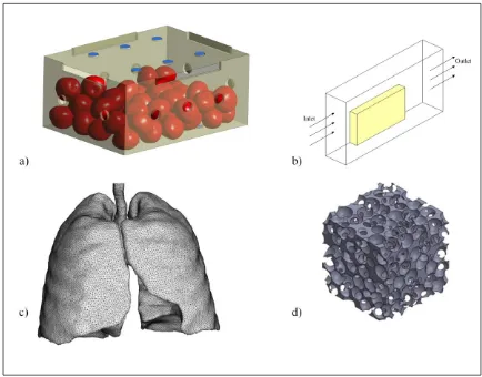
Figure 1.1: Applications of porous media including a) modeling of tomato stacks (taken
from Elhalwagy, Dyck and Straatman [1]); b) convective drying of an apple slice; c)
modeling of the human lung (taken from DeGroot and Straatman [2]); d) modeling of
Graphite foam(taken from Dyck and Straatman [3]). ... 2
Figure 1.2: Porous media micro- and macroscales. The left panel depicts a microscopic representation of Porous media with liquid trapped inside the solid’s micro-pores while the right panel shows the continuum or macroscale equivalent perception. ... 3
Figure 1.3: Schematic showing a microscopic representation of a moist Porous material. 6 Figure 1.4: Heat and mass transfer coupling in CFD studies of Fluid/Porous domains. .. 11
Figure 1.5: Schematic of a representative elemental volume (REV) illustrating the different phases and their volume averages. ... 23
Figure 1.6: Conjugate Fluid/Porous/Solid domains. ... 36
Figure 1.7: Finite volume CFD discretization in structured orthogonal frameworks. ... 36
Figure 2.1: A discrete conjugate Fluid-Porous domain. ... 58
Figure 2.2: Illustration showing the different constituents in the porous region and the simplification of the problem. ... 60
Figure 2.3: Schematic showing a spherical solid holding liquid water within its micro-pores subjected to a stream of moist air. ... 66
Figure 2.4: Moisture circuit analogue at the macroscopic interface. ... 71
xiii
Figure 2.6: Temporal variation of the coal bed averaged liquid mass fraction compared to
the experimental results reported in Stakić and Tsotsas [33]. ... 81
Figure 2.7: Temporal variation of the coal bed averaged solid particle temperature
compared to the experimental results reported in Stakić and Tsotsas [33]. ... 81
Figure 2.8: Axial variation of the centerline value for liquid moisture fraction, particle and
void temperatures at different simulation times... 82
Figure 2.9: Schematic and grid used for simulation of drying of an apple slice. ... 84
Figure 2.10: Apple diffusivities as a function of the liquid moisture ratio. ... 86
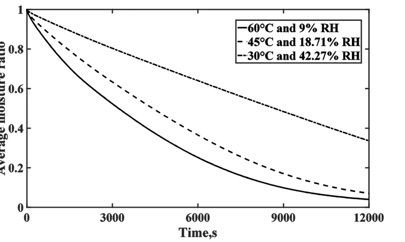
Figure 2.11: Temporal variation of the averaged apple moisture ratio for different inlet
velocities compared to the experimental results of Velić et al. [35]. ... 87
Figure 2.12: Temporal variation of the averaged apple moisture ratio for different inlet
velocities accounting for the advective effects; comparison to the experimental results of
Velić et al. [35]. ... 88
Figure 2.13: Temporal variation of the averaged apple moisture ratio as a function of inlet
airflow relative humidity for 1.5 m/s inlet velocity. ... 89
Figure 2.14: Temporal variation of the averaged apple moisture content as a function of
the inlet temperature at a fixed inlet specific humidity for 1.5 m/s inlet velocity. ... 90
Figure 2.15: Contour plots for liquid apple moisture spatial variation along the
domain-cutting symmetry planes at different time instances. ... 91
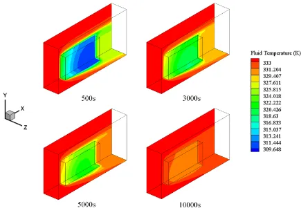
Figure 2.16: Contour plots for fluid temperature spatial variation along the domain-cutting
symmetry planes at different time instances. ... 92
Figure 2.17: Contour plots for solid temperature spatial variation along the domain-cutting
xiv
Figure 2.18: Simulation setup for the mineral plaster dehydration process. ... 93
Figure 2.19: Mineral plaster diffusivities as a function of the moisture ratio... 96
Figure 2.20: Variation of the average moisture ratio as a function of the drying time for mineral plaster. ... 96
Figure 2.21: Temporal variation for the distribution of liquid moisture content of mineral plaster (a scale with four decimal places was necessary to observe the moisture fronts). 97 Figure 2.22: Relative humidity distribution at 1 hour of simulation time for mineral plaster. ... 97
Figure 2.23: Distributions of temperatures at 1 hour of simulation time for mineral plaster. ... 98
Figure 3.1: Schematic of a Fluid/porous transition showing the differences between a micro- and macroscopic interface and low and high permeability porous regions (moist air is white, liquid is blue and solid is grey). ... 113
Figure 3.2: Shear stress at a macroscopic interface. ... 129
Figure 3.3: Moisture resistance analogue for the macroscopic interface. ... 129
Figure 3.4: 2D flow numerical setup around and through a porous obstruction. ... 138
Figure 3.5: Normalized pressure contours for a 2 m/s flow over Potato and apple porous obstructions with the use of EWT. ... 140
Figure 3.6: Axial velocity contours for a 2 m/s flow for cases of different porous properties and different interface treatments. ... 141
xv
Figure 3.8: Normalized TKE contours for a flow of 2 m/s with different porosities and
interface treatments (Scale is cut of above the reported maximum to show the
penetration/dissipation of turbulence). ... 143
Figure 3.9: Normalized turbulence dissipation contours for a flow of 2 m/s with different
porosities and interface treatments (Scale is cut of above the reported maximum to show
the penetration/dissipation of turbulence). ... 144
Figure 3.10: Velocity and turbulence contours of an EWT potato case of 10 m/s (Scale is
cut of above the reported maximum to show the penetration/dissipation of turbulence).
... 146
Figure 3.11: Transverse profiles for flow and turbulence across the shear macroscopic
interface for x=0.75 l along the porous slice for a 2m/s potato case and different interface
treatments. ... 147
Figure 3.12: Numerical setup for turbulent convective drying of a slice of produce. .... 148
Figure 3.13: Diffusivities as a function of the moisture ratio. ... 150
Figure 3.14: Moisture ratio versus time. ... 151
Figure 3.15: Contour plots for produce liquid moisture spatial variations at different time
instances. ... 153
Figure 3.16: Contour plots for fluid temperature spatial variations at different time
instances. ... 154
Figure 3.17: Contour plots for solid temperature spatial variations at different time
xvi
List of Nomenclature
𝐴 area, m2
𝐴𝑓𝑠 specific interfacial surface area of porous media, m-1
𝑎𝑖 CFD active coefficient of control volume i
𝑎𝑊 water activity
𝐵 Spalding mass transfer number
𝐵𝑖 Biot number
𝑏𝑖 CFD active source term of control volume i 𝑐𝐸 inertia coefficient of porous media
𝑐𝑝 specific heat at constant pressure, J/kg. K
𝑐𝑝𝑠 specific heat in the solid phase, J/kg. K 𝐶𝑇, 𝐶𝑚, 𝐶𝑇1, 𝐶𝑚1 heat and mass transfer correlation constants
𝐶𝑘, 𝐶𝑙, 𝐶1𝜀, 𝐶2𝜀, 𝐶𝜇 turbulence modelling constants
𝐷 binary diffusivity coefficient, m2/s 𝐷 Coal particles bed diameter, m 𝑫 deformation tensor
𝑑𝑃 Porous media particle diameter, m
xvii
𝐻 channel height, m ℎ specific enthalpy, J/kg ℎ height of porous region, m
ℎ𝑓𝑔 latent heat of vaporization at 0°C, J/kg
ℎ𝑓𝑠 interfacial heat transfer coefficient in porous media, W/m2.K
ℎ𝑓𝑠𝑚 interfacial mass transfer coefficient in porous media, m/s
I the unit dyadic
𝑖 species counter
𝐽𝑣′′𝑖𝑛𝑡. overall vapor mass transfer flux at fluid/porous interface, kg/m
2.s
𝑘 thermal conductivity, W/m.K, turbulent kinetic energy, m2/s2
𝐾 permeability of porous media, m2
K phase ratio
𝐿 Porous media length, m
𝑙 REV size, m
𝑀 overall moisture concentration, kg/m3
𝑚 mass, kg
𝑚̇ mass flow rate, kg/s
N number of neighbors of a CFD cell
xviii
𝑁𝑢 Nusselt number
𝑃 pressure, Pa
𝑃𝑖 turbulence production of i
𝑃𝑟 Prandtl number
𝑄𝜑𝑃 CFD explicit part of the source of 𝜑 at control volume P 𝑞𝑖𝑛𝑡.′′ overall heat transfer flux at fluid/porous interface, W/m2
𝑅𝑖 gas constant of i, J/kg. K 𝑅 mass transfer resistance
𝑅𝑒 Reynolds number
𝑅𝐻 relative humidity
𝑅𝜑𝑃 CFD linearized part of the source of 𝜑 at control volume P 𝑆 source in a transport equation
𝑆𝑐 Schmidt number
𝑆ℎ Sherwood number
𝑇 temperature, K
𝒕 shear unit tangent vector
𝑡 time, s
𝑈 Inlet velocity, m/s
xix
𝑢𝑖𝑛𝑡 slip shear velocity component at the fluid/porous interface, m/s
𝐯 fluid velocity vector [=(𝑢, 𝑣, 𝑤)], m/s
𝑉 volume, m3
𝑥 distance in axial direction, m
𝑥 phase index
𝑦 distance in y-direction , m
𝑌 mass fraction
𝛼 vaporization energy apportioning factor 𝛼𝑥 volume fraction of 𝑥
𝛽 enhanced vapor diffusion factor 𝛤𝜑 diffusion coefficient of the entity 𝜑
𝛿𝑑𝑖𝑓𝑓. significant liquid diffusion thickness, m
𝜅 Von-Karman constant (= 0.41) 𝜇 dynamic viscosity, N.s/m2
𝜇𝑡 turbulent eddy viscosity, N.s/m2
𝜁 dry solid layer’s diffusion resistance altering factor 𝜎𝑘 turbulent Prandtl number for 𝑘
𝜎𝜀 turbulent Prandtl number for 𝜀
xx
𝜏 reciprocal of the turbulence time scale, s-1 𝜏𝑖𝑛𝑡. shear stress at the macroscopic interface, Pa
𝜌𝑠 Solid density, kg/m3
𝜌𝑓 density of fluid mixture, kg/m3
𝜖𝑖 turbulence destruction of i
𝜀 Porosity (chapter 2), turbulent energy dissipation (Chapter 3), m2/s3 𝜂 dimensionless length scale for calculation of 𝜇𝑡in enhanced wall
treatment
𝜆𝑥 thermal conductivity of phase 𝑥, W/m.K (only for turbulent flow)
𝜙 porosity (only for turbulent flows) 𝜑 An entity of interest
𝜑̅ time-average of 𝜑 𝜑′ time fluctuation of 𝜑
〈𝜑〉 extrinsic volume-average of 𝜑
〈𝜑〉𝑥 intrinsic volume-average of 𝜑 for phase 𝑥
𝜑̃ volume deviation of 𝜑 〈𝜑̅〉 volume-time-average of 𝜑
xxi
subscripts and superscripts
𝑎 air
𝑐𝑜𝑛𝑣. convection
𝑑𝑖𝑓𝑓. diffusion
𝐸 CFD east neighboring cell 𝑒 CFD east integration face
𝑒𝑓𝑓 effective property in porous media
𝑓 fluid
𝑓𝑙 fluid side of interface 𝑓𝑠 interfacial
HT Heat transfer
𝑖𝑛𝑡𝑒𝑟𝑓. macroscopic interface
𝑚 mass transfer (subscript), exponent of Reynolds number in heat and mass transfer correlations (superscript)
MT mass transfer
𝑚𝑎𝑐𝑟𝑜. at fluid/porous interface (macroscpoic interface)
mod,t modified by turbulence
n exponent of Prandtl number in heat and mass transfer correlations
xxii
𝑃 control volume (𝑃) 𝑝𝑜𝑟 porous side of interface
𝑠 solid
𝑠𝑎𝑡 saturation
𝑠𝑜𝑙. solid particle surface
st solid matrix
𝑇 Heat transfer
𝑣 vapour
𝑤 water
𝛤𝑖 profile exponent of the dimensionless wall function for equation i 𝛾 general CFD integration face
+ superscript associated with non-dimensional wall function variables
Abbreviations
CFD Computational Fluid Dynamics
DNS Direct Numerical Simulations
EWT Enhanced Wall-like Treatment
xxiii
PIV Particle Image Velocimetry
RANS Reynolds-Averaged Navier-Stokes
REV Representative Elementary Volume
RNG Re-Normalized Group
RSM Reynolds Stress Modelling
SAT Spatial Averaging Theorem
SST Shear Stress Transport
Chapter 1
1
Introduction
1.1
Background and scope to contribution
This thesis is concerned with the development of a reliable, time efficient and physically
dynamic modelling approach that characterizes fluid flow processes around and through
porous media, predicting heat and mass transfer locally and globally for different
processes, materials and physical conditions.
1.1.1 General Background
Porous media are abundant in everyday life. To name some: particles, grains, sands, soil,
fabrics, bricks, metal foams, produce, food stacks, catalytic honeycombs, biological tissues
and even liquid mists and sprays are all of porous nature, involving variety of sizes and
physical properties. Thus, a wide range of engineering processes and industries are
interested in fluid flow, heat and mass transfer around and through these media. Examples
include, porous metal foams, porous heat sinks, air conditioning, drying (fabrics,
construction materials and foodstuffs, etc.), food cooling and storage, food quality
forecasting and ripening, prediction of undersoil smoldering, forest fires, planetary
boundary layer through rough terrains and forests, engine catalytic converters and porous
burners, some of which are included in Fig. 1.1. This widespread application within these
diverse areas of engineering, necessitates a thorough understanding of the different
physical processes like fluid flow, heat and mass transfer around and through porous media
to facilitate engineering design and analysis and accelerate the process of development.
For the purpose of this work, the term “porous media” refers to structures that are
comprised of solid and fluid constituents in a relatively homogeneous distribution such that
it may be considered a continuum of both. While a porous material may be permeable or
impermeable, the interest herein is directed towards fluid-permeable porous materials,
where air, water or some other fluid can pass through the solid structure under the influence
of a pressure gradient. Examination of the solid and fluid constituents (or phases) of the
If one zooms in and considers the internal structure of a porous medium, the length scale
of some physical process may be characterized by the distance between two chunks of
solid, or the diameter of a pore or void space, or it can be the averaged size or diameter of
individual solids (particles, ligaments, etc.), or any other suitable dimension at this
microscale. The presence of other forms of matter may also be observed inside what are
characterized as the solid or fluid constituents of the porous structure; consider, for
example, water vapor in air or liquid water trapped within the solid constituent in tiny
interconnected micro-pores (see left panel of Fig 1.2). The presence of temperature
Figure 1.1: Applications of porous media including a) modeling of tomato stacks (taken from Elhalwagy, Dyck and Straatman [1]); b) convective drying of an apple
gradients or species concentration gradients between the two phases causes heat and mass
transfer on this local (sub-micro) scale as well.
Figure 1.2: Porous media micro- and macroscales. The left panel depicts a microscopic representation of Porous media with liquid trapped inside the solid’s
micro-pores while the right panel shows the continuum or macroscale equivalent perception.
Depending on the microscale and the geometric nature of the solids or the voids within a
porous medium, the physics of the fluid flow or any transfer of heat or mass (e.g. moisture
evaporation/condensation) can differ significantly and hence, the resolution of different
phenomena is very important on this small scale.
Zooming out, the most prevalent length scale is related to the geometric size of the entire
porous medium. On this macroscale, bulk flow variations and pressure drop, and bulk heat
and mass transfer is often the goal of net characterization of the physics. Both scales
interact considerably and cause different possible behaviors (see Fig 1.2 for porous media
scales). Another aspect of interest for physical studies is the different interactions at the
interface between the surrounding fluid region and the porous medium; this is often the
most difficult part of modelling a process of fluid, heat or mass transfer. The interface is
also often complicated by the heterogeneity present in the structure of porous media, i.e.
rapid changes in porosity, and the variations of the fluid flow behavior due to shear and
obstruction. For heat and moisture transfer, other factors like conduction and diffusion
enhancement/inhibition, fluid acceleration/deceleration, phase change, capillarity, surface
tension effects, etc., interplay together to pose modelling challenges at interfaces under
already-complicated physics. Instantaneous time-local variations in the flow velocity,
temperature or moisture concentration with time are of a small time scale and transient
physical phenomena observation (e.g. drying) is of a larger time scale. Hence, in addition
to the presence of multiple length scales, processes are affected by multiple time scales as
well.
Characterization and study of different phenomena in porous materials often relies on
empiricism and is based on some insight into the physical processes. To this end,
experimental studies carried out on a bulk scale can quantify the overall drying rate, heat
transfer, flow resistance, etc., through a permeable porous material. A more in-depth
analysis often depends on numerical simulations based on computational fluid dynamics
(CFD) and done at the pore-level. Such analyses can take the place of costly and
sophisticated experimentation conducted to resolve the physics inside complex structures
subject to multiple length and time scales. Modeling the porous structure at the pore-level
depends on resolving the microscale and hence, phenomena is characterized for all voids
and particles/ligaments inside the porous material, which can also be prohibitive and
time-expensive. A second computational approach is to resolve only the macroscale (i.e.
continuum approach) but with upscaling mathematically the microscale information using
volume-averaging. Within this approach, with respect to heat and mass transfer, a simple
technique is to consider a single temperature and/or mass fraction to characterize a small
representative region of porous material, thereby enlisting the assumption of local thermal
and mass equilibrium. This equilibrium approach, while successful when this homogeneity
is physically acceptable, is of restricted applicability to different classes of problems in
which the equilibrium is partially or fully unachieved. Separating the two phases with
respect to heat and mass transfer is a solution to this problem and is of an affordable time
expense however, it requires a reliable and accurate microscopic phase exchange modeling.
In engineering applications and designs, porous materials are often combined with other
solid materials and immersed in a fluid environment to form conjugate domains of
fluid/porous/solid regions. Across the clear fluid/porous transition, different modeling
approaches have been considered including forcing a gradual change of obstruction
regions, i.e. either model one region and link it to an empirically estimated effect to the
other, or, model one region at a time and obtain the result from this region then use it to
carry the interface effect on to the second one (indirect coupling approach). These three
approaches are of additional time cost and/or loss of accuracy. The conjugate approach
depends on linking the two regions in a single simulation step and ending up with a full
characterization of both fluid and porous regions which is time-efficient. While the
approach is challenging, considerable success is achieved with room for further
development. The process of coupling turbulent flow through both regions in particular is
an active area for improvement especially to achieve capability for modeling different
ranges of porosity that allow turbulence to penetrate/dissipate into the porous region
depending on the level of flow resistance.
1.1.2 Scope
Industrial modelling of general heat and mass transfer and/or drying/rehydration (i.e.
heat-affected moisture transfer) in conjugate fluid/porous/solid domains has depended on the
above-mentioned design tools and basic CFD studies. Departure from these simple,
accuracy-limited, empirical ad-hoc or case-specific techniques has been long under
development. It is interesting to mention that to-date (to the best of the author’s knowledge)
no commercial CFD software contains a generic, accurate, conjugate fluid/porous/solid,
time-efficient and physically dynamic; capability for modelling combined flow, heat and
mass transfer. The research community is focused on either in-house coding, coupling
between different softwares/codes for simulating different regions and is heavily loaded
with the different above mentioned empirical or non-generic assumptions. Few studies in
the recent years have made progress with conjugate and physically-based CFD for these
problems. The present work is a basic step towards the development of a generic,
highly-coupled and physically-dynamic approach. The scope herein is directed towards the void
areas in CFD literature, as will be shown shortly, where heat and mass exchanges locally
(interstitially) and macroscopically (across regional interfaces) are either:
- Overlooked
- Formulated with limited reactivity to dynamic physical changes and modes of flow, heat and mass transfer
The approach taken herein is a compromise between very detailed physical modelling for
multiple length and time scales, empiricism and time efficiency and it provides alternatives
that are capable of solving the above mentioned problems. The resulting work provides a
framework that is generic, conjugate, simultaneous for all regions, and physically dynamic
with a significant reduction of empiricism which provides a starting point for further
development.
The rest of this chapter focuses on reviewing the modelling state of the art, objectives of
thesis, research methodology (i.e. averaging techniques, model development background,
necessary terminology and numerical discretization) and closes with the thesis outline.
Figure 1.3: Schematic showing a microscopic representation of a moist Porous material.
1.2
Literature survey
1.2.1 Modelling heat and mass transfer of moist porous materials
A moist porous material is a porous material that includes four phases within it. The fourphases are, solid matrix or particles, void space including moist air (dry air and water
with both air and solid phases, and the bound water which is liquid water embedded inside
the solid constituent and is not free to move or evaporate (See Fig. 1.3). Drying and
rehydration studies are focused on modelling the heat and mass transfer techniques for
moist porous materials. One school of practice was established on the work of Luikov
[4-5] which tackles the problem from a thermodynamic point of view and does not depend on
macroscopic averaging techniques but on a phenomenological approach. It also
standardizes the inclusion of the Soret and Dufour effects (i.e. mass and heat transfer due
to temperature and species concentration gradients, respectively). This school often refers
to moist porous media as capillary-porous and hence it depends highly on characterizing
moisture transfer by capillarity. The approach is usually applied in CFD by solving the
capillary pressure as a transport variable [6-7] and utilizing a convection term in the liquid
transport equations to represent moisture travel macroscopically. The method is of wide
use for construction materials. The approach while successful, is non-generic due to its
specificity to one certain form of moisture presence (i.e. liquid only) and the fact that it
solves the capillary pressure to characterize moisture transfer instead of the mass fraction
or species density which are the real conserved variables in this case. Another school of
work is Whitaker’s [8-9]. His work started by taking the analogy between transport in space
and time and coming up with the concept of volume averaging following Reynold’s
approach for time averaging. The approach ended up by obtaining all the flow, heat and
mass transfer volume-averaged forms of conservation equations for the main three phases
i.e. air, liquid and solid. The drawback was the very complicated form of the transport
equations and the mathematically complex equations of closure [10-11] that need to be
solved for a useful utilization of the approach. Closure may also be sought using
microscopic data or void level simulations [3, 12]. Special interest has been given to the
bound water phase in the literature. Some researchers solved an individual transport
equation for this phase separating it from the free liquid phase [13]. Others included them
in one equation, but they introduced special terms for diffusion [14] to characterize the
different phases e.g. Arrhenius-type expressions or entropy-based approximations to model
the gradual freeing of the bound water by heating [15]. Moist porous materials are also
categorized to hygroscopic and non-hygroscopic materials [16]. Where a hygroscopic
based on gradual variation of diffusivity or gradual variation of moisture-bond energy e.g.
Food [16] while, non-hygroscopic materials are of reduced affinity for moisture. They
contain limited amount of free moisture and the moisture-bond to it for the bound phase is
very difficult to free i.e. a relatively high diffusivity in the beginning of drying that drops
several orders of magnitude in a very short drying time until the material is of nearly
neglected diffusivity [6] e.g. some building materials. For both types of materials, the
mechanism of moisture transport depends on diffusion, capillarity and surface tension
effects [4, 6, 16]. It is also common in the literature to neglect the void phase presence
inside the moist porous material and model only liquid and solid phases [17-18]. The
approach is again non-generic as it neglects the mechanism of vapor diffusion and the
presence of vapor moisture which is not realistic in a lot of cases. Other studies tend to
include vapor diffusion mechanism but they incorporate it within a single equation for
liquid and vapor [6-7, 14] which is better physically however the segregated species
modeling offers more general applicability and it also allows modelling of local phase
exchange.
1.2.2 Phase-heat and mass interstitial exchange
Generally, heat and mass transfer inside porous media is categorized to equilibrium and
non-equilibrium approaches. An equilibrium approach depends on considering one
homogeneous presence of heat and mass transfer for all the phases i.e. one discrete equation
for temperature and another for moisture concentration or mass fraction only per each
control volume (elaboration will follow in a subsequent section). While non-equilibrium
approaches separate each phase’s characterization into one equation i.e. a number of
equations equal to the number of phases per control volume. The first approach is widely
used in the literature [17-20] however it does not model the phase exchange processes
because it considers the transport for the sum of the phases. Our discussion here is relevant
to the second approach. Some studies resorted to close the interstitial phase exchange using
empirical adjustment [21-22] to account for different modes of heat and mass transfer
locally e.g. forcing a mass transfer coefficient of exchange to decrease empirically near the
dry out [22]. Studies of packed beds or grain drying [23-27] gave their focus to the
particle has either been assumed as fully saturated with vapor [22], or a thermodynamic
equilibrium approach is invoked (more details about thermodynamic equilibrium will
follow) to allow a relation between solid surface relative humidity and water activity of the
solid particle to form [23-24]. In this approach, the liquid moisture content inside the solid
is correlated to the surface vapor concentration on the fluid/solid interface, allowing a
driving potential for mass transfer to link both phases using an analogue of Newton’s law
of cooling [22-24] in which a local interstitial mass transfer coefficient is estimated based
on the physics of the flow and the geometric structure of the porous material. This
thermodynamic equilibrium expression based on this definition has some limitations close
to drying out and does not consider an explicit introduction of the resistance to mass
transfer inside the solid constituent. Another problem with the analogue of Newton’s law
of cooling is that it considers only the diffusive effects in the boundary layer for vapor
transport without inclusion of advective effects [17, 22] i.e. Stefan flow. Other studies has
considered both a thermodynamic equilibrium approach outside of the solid constituent
and a diffusion resistance model on the inside. They either solved an equation inside the
solid particle for the solid side’s resistance [25-26] or empirically estimated the solid side’s
resistance from drying kinetics data [27]. Both types of treatments however preserved the
thermodynamic equilibrium at the interstitial interface. In a different case, the drying
kinetics data were solely used for representation of the phase exchange mass flux without
including a fluid side expression [28]. Most of the grain and particle drying studies were
applied on one or two dimensional models [13,27-29] mostly because of the complicated
local phase coupling approaches, which is not feasible for implementation in cases of high
three dimensionality.
The second aspect regarding local phase exchange concerns with the phase exchange
energy (i.e. energy accompanying species transport across phases). This energy is mostly
representing the latent heat of vaporization for moisture. It is common for applications of
evaporative cooling or cases where deviation from thermal equilibrium is minimal [22, 30],
to apportion this energy (i.e. withdraw it) completely to the fluid phase. In other cases
where the liquid is mostly embedded inside the solid (e.g. packed beds), the practice was
to apportion it completely to the solid phase [24, 27-29]. While both assumptions are
The physics of vaporization dictates that when liquid is placed at the interface between two
phases, it may vaporize and travel between them based on whichever source that can supply
the vaporization energy i.e. for free liquid water both phases may contribute to the
vaporization heat in different proportions [31].
1.2.3 Coupling across fluid/porous interfaces
Now, the heat and mass transfer coupling between a surrounding fluid region and a moist
porous region is reviewed. The fluid/porous regions’ linking is achieved either, with an
overall empirical/semi-analytical assessment e.g. a drying kinetics technique, a single
phase approach which solves single equation of heat and another for mass inside each CFD
cell, an uncoupled phase approach that solves the different regions without direct coupling
or a conjugate technique that directly couple the different phases. In the first approach, the
overall phenomenon is characterized without local variations i.e. no discrete or CFD
approach is utilized. This overall behavior is determined based on a drying experiment for
a certain specimen of the material of interest and/or a semi-analytical approach that
represents an equation for the overall diffusion inside the moist material and its correlation
with time or utilizes an Arrhenius-type expression to correlate the kinetic data to overall
moisture content and temperature [32-36]. The second category solves only one equation
for temperature and one other equation for the overall moisture in the porous region i.e.
utilizes an equilibrium approach within the porous media [17-20] (See Fig. 1.4 for a
complete description of the different types of CFD regional coupling). While these studies
provide a discrete CFD solution, they utilize an empirical estimate of overall heat and mass
transfer coefficients at the macroscopic interface i.e. clear fluid/porous interface that carry
the effect of the surrounding fluid region on the porous region. These empirical estimates
are based mainly on Nusselt and Sherwood number correlations existing in the literature.
This single phase approach also provides an overall characterization of the heat and mass
transfer however, it is restricted by the applicability, accuracy and case-specificity of these
empirical estimations. It may also suffer from the non-equilibrium errors within the porous
Figure 1.4: Heat and mass transfer coupling in CFD studies of Fluid/Porous domains.
The third group of studies utilize an uncoupled phase technique which means that both, the
numerically/analytically within them however no interface coupling is present [37-39]. The
linking is achieved by using the discrete solution of the fluid region to estimate an interface
heat transfer coefficient and utilizing the heat and mass transfer analogy to deduce the
corresponding mass transfer coefficient. A convective boundary condition is then set from
both transfer coefficients to solve the heat and mass transfer inside the porous region.
Figure 1.4 illustrates the process. This technique utilizes equilibrium approaches inside
the porous region as well. The last approach for coupling is a conjugate approach in which
the full characterization for heat and mass transfer is carried out within both regions. This
approach is subdivided to explicit and implicit subcategories. The explicit technique [6,
40] depends on separating the numerical solution of both regions in a way that the interface
side coupling is set in the discrete form as a boundary condition and hence multiple
iterations or overlapping time steps have to be performed in which multiple explicit updates
need to be made for the interface coupling fluxes. A way to reduce these multiple iterations
is to reduce the time stepping size so that one update is enough per time step in which the
information is carried from the fluid region to the porous region. An obvious disadvantage
for this approach is the computational expensiveness and potential stability problems that
may require adaptive time stepping to overcome [40]. Few studies have achieved an
implicit form of coupling in which both regional equation sets are solved simultaneously.
Of these studies a two dimensional approach that is based on using a stream function for
the fluid flow is notable [41]. The approach while successful is restricted to two
dimensional cases only. A second study achieved this form of coupling with the use of
non-equilibrium heat and mass transfer inside porous media however they utilized ad-hoc
resistance-altering coefficients for mass transfer coupling at the fluid/porous interface that
varied from a simulation to another which is case-specific [30]. The resistances of heat and
mass transfer implicit coupling are shown in Fig. 1.4.
1.2.4 Turbulence within porous media
Turbulence plays a major role in heat and mass transfer processes related to porous media
hence, it is very important to study the different approaches utilized for modeling within
the porous material and across the macroscopic interface. The present section is concerned
The models were single equation models that resolved the turbulent kinetic energy (TKE)
and utilized a mathematical expression for its dissipation rate rather than adding another
equation. The first version of this expression depended on four empirical constants [42]
and the enhanced version eliminated two of them [43]. Generally, the approach simplified
the porous media flow modeling by using the Darcy equation with its Forchheimer-added
drag resistance with neglecting convection and diffusion transport. It also carried the
turbulence effect into heat transfer by using a turbulence intensity-dependent Nusselt
number correlation. The main direction of work in the literature focused on two equation
modelling, following the direction of volume averaging the time averaged k-ɛ equations.
One group of studies attempted the time-volume-averaging process i.e. Double
decomposition (discussion will follow in a subsequent section), based on a definition of
TKE that time averaged the square of the volume-averaged velocity fluctuation 𝐯′ [44-47]. The definition caused the order of the averaging processes to change the final output for
different cases and it also lacked the inclusion of a volume-deviation-time-fluctuation term
for the TKE and its dissipation rate. A more general definition was introduced later
[48-49] that squared the velocity fluctuation first and then performed the two averaging
processes i.e. the double decomposition. This definition included the above mentioned
volume-deviation-time-fluctuation term and resulted in an immaterial order of integration.
Another introduced definition added to the last one, another term that relates to the porous
media dispersion [50-51] to form a TKE equation that resolves the velocity variations
macroscopically for time and space integrations. Based on these different definitions for
TKE, three different attempts [48, 49, 51] for closure of a k-ɛ model were performed inside
porous media using pore level simulations and ended up successfully adding three different
forms of drag terms in the k-ɛ equations. All three forms are suitable for macroscopic
modeling and may be closed for different variations of void level simulations [12]. More
advanced modeling have also been carried out. Reynolds stress modeling (RSM) has been
utilized [52-53]. While it has been used without any additional change inside porous media
for one study [52], macroscopic scaling and closure has been achieved as well [53]. Also,
multiple-equation versions of the k-ɛ model have been created in the literature for cases
that added a separate two equations of TKE and its dissipation to characterize dispersive
dissipation into separate k-ɛ sets [55]. The three-way splitting approach of k and ɛ have
been developed later into a second moment closure approach as well [56]. A low Reynolds
number model have also been developed based on a Lam-Bremhorst version that utilized
direct numerical simulations (DNS) inside porous media for validation [57]. Generally, all
the turbulence modeling work inside porous media has been successful however, due to
the complication of characterizing the additional dispersive and tortuous effects to an
already existing random characterization for turbulence for any of the above modeling
frames, most of the models were too complex and the multiple equation models were too
computationally expensive rendering the standard double decomposed versions of the k-ɛ
model to be the most useful.
In regards to turbulent heat and mass transfer studies, two significant areas of work are
concerned with drying and food stacking, respectively. In the first category of work,
significant amount of the studies depended on the same assumptions that were utilized
inside porous media for laminar flows (see sections 1.2.2 and 1.2.3). They included two
equation models of turbulence with standard wall functions to account for boundary layer
effects at the macroscopic interface with the exception of few studies. A standard version
of k-ɛ model with standard wall function was utilized by, to name a few, Curcio et al. [58]
(parallel flow over food sample, continuity heat and mass transfer flux boundary condition
and thermodynamic equilibrium at fluid/sample interface with a non-porous equilibrium
approach inside the sample), DeBonis and Ruocco [59] (jet impingement over a general
wet protrusion, non-porous approach, non-equilibrium inside the protrusion with lumped
vapor/liquid diffusion into a single diffusivity and an Arrhenius expression for macroscopic
interface evaporation) and Caccavale et al. [60] (parallel flow over a general wet protrusion
utilizing the same approach as [59]). Ateeque et al. [61] utilized a k-ω SST two equation
model for modeling the flow around a potato slice based on testing different two equation
models for a backward facing step as they considered the separation of the flow and
re-attachment as the most significant turbulent behavior for such a kind of flow. For turbulent
heat and mass transfer, they considered a non-porous/non-conjugate model that relied on
surface transfer coefficients for coupling at the fluid/slice interface. The turbulence effect
was incorporated for heat and mass transfer via the flow-spatially dependent surface
downstream one. Another approach for brick drying by Van Belleghem et al. [7], used a
realizable k-ɛ model with a low-Reynolds number region at the macroscopic interface
instead of a wall function. The heat and mass transfer approach depended on the capillary
pressure and incorporating both vapor and liquid transports into one equation inside the
drying sample with an empirical specification of the transfer fluxes at the air/brick
interface. Studies in this category of work did not consider porosity effects, turbulence
inside the drying samples and suffered from the same case-specific empiricism at the
macroscopic interface and the time consuming coupling between air heat and mass transfer
and the inside of the drying sample and/or equilibrium assumption’s inaccuracy. A notable
study was conducted by Defraeye et al. [62]. They considered flow around an apple slice
and assessed multiple turbulence models in the prediction of drag coefficient, Nusselt
number, Separation angle and back reciriculation length. Models included different types
of k-ɛ, k-ω and RSM. In interface adjacent regions, low Reynolds number modelling as well as standard wall-functions were utilised. They concluded that the k-ω SST with low
Reynolds number modeling behaves the best in terms of the above mentioned criteria. The
drawback was dependence on fine meshes in this case. It is also noted that switching from
low-Re modeling to standard wall function was a highly pronounced effect on the k-ω SST
as compared to the same switch for a k-ɛ model.
In the second category of work, porosity inside the food stacks or boxes could not be
neglected and hence, turbulence was mostly switched on inside the porous region. To
characterize this macroscopic porosity, void level simulations were mainly utilized to
provide closure for the macroscopic porous models. The closure path either depended on,
empiricism [63], sensitivity analysis for different closure parameters of flow, heat and mass
transfer [64], experimental evidence [65] or physical analysis utilizing a representative
elementary volume (REV) and averaging the microscopic information through it [66-67].
In these studies the RNG k-ɛ [63, 68], k-ω SST [64-67] and RSM [69] were utilized. A
choice of a model was mainly based on assessment of different models based on the
average error between the experiments and CFD predictions of velocity [66] and
temperature [65]. A drawback was that the deviations of different turbulence models near
the fluid/porous interface was not considered. One study by Tutar et al. [68] came to a
heat and mass transfer and that other effects like presence of three dimensionality and
changing the flow rate are more significant. The disadvantages for this category of studies
was the absence of interest in closure of additional porous media terms in the turbulence
models and the lack of an investigation of the fluid/porous interface mathematics for
coupling turbulence across both regions i.e. all of the above studies depended on the
technique that is available in the utilised commerical software ANSYS FLUENTTM [70]
plus forcing a switch off for turbulence in some regions (porous and fluid)[63].
1.2.5 Turbulence coupling across macroscopic interfaces
Due to the different natures of the volume averaged equations of porous media and the
clear fluid equations, it is important to have a valid coupling approach of turbulence
between both regions. Such a process is reliant on an understanding of the physical changes
across the transition between both regions. One group of studies focused on utilizing
different turbulence models for the macroscopic interface-adjacent layer from the clear
fluid side and the free stream region. Such an approach was utilized with a k-l model near
the interface, a k-ɛ model in the free stream and a compatibility mathematical condition in
between [71]. The work utilized a dimensionless fully developed pipe flow around a porous
layer and a Brinkman-Forchheimer-extended Darcy equation through it. Another version
of the work utilized a Cebecci-smith two-layered turbulence model [72-73] and analyzed
the thermal dispersion process inside the porous region [73]. The main disadvantage was
relying on a dimensionless analytical expression for the pipe flow, rendering the findings
to be case-specific and not generally applicable for other CFD studies. One other study
utilized an Analytical wall function [74] for the flow adjacent to a porous region and
matched it to an approximation of the Darcy equation solution inside it. Again, this
approach was not possible to generalize on other CFD studies. Another work used enough
refinement to well capture the viscous layer without modelling and utilized simple
turbulence modeling (Prandtl mixing length, Han-Van Driest and Baldwin-Lomax) on the
outside region [75] which is considered an over-simplification. Multiple coupling of
different models have been utilized by Beyhaghi et al. [76] with a pore-network model (for
fluid flow and its moisture coupling) inside the porous region, FLUENTTM [70] for clear
process. A no-slip condition was imposed at the macroscopic interface. This group of
studies neglected turbulence inside the porous region which is a significant loss of
generality.
A second school of work depended entirely on void-level CFD simulations for
characterizing the fluid/porous transition. They utilized case specific geometries like group
of rods [77] or cubic blocks [78] and their interaction with clear fluid regions with no need
for mathematical interface treatments. Sophisticated modeling has been carried out as well
in which both a large eddy simulation (LES) or (DNS) is utilized for void level simulations
on clear fluid transition to inline/staggered blocks/spheres and continuum approaches for
porous media with the same geometry. Jin and Kuznetsov [79] used DNS and volume and
time averaged the data to form a basis for comparison to continuum modeling. They
concluded that zero equation modeling is enough inside the porous region and turbulence
scale is restricted by the pore size. Forcing a gradual change of porosity between the fluid
and porous region for the continuum modeling was deemed useful as well [80-81]. The
approach enabled using one form of equations for both regions and a turbulence coupling
mathematical condition was not necessary. Also, PIV experiments outside the porous
region and LES simulations on the inside of it were utilized with the gradual porosity
transition technique to develop a four-equation multiscale k-ɛ model that was successful
for analyzing the turbulence within and across the porous region [81]. One may comment
that these sophisticated models while capable, they are not general, require extremely fine
meshes and have long computational times.
A successful and economic approach for devising a mathematical condition for turbulence
across fluid/porous interface was reported [82-83]. The approach utilized a jump condition
at the interface for momentum [84] with a continuity condition for k and ɛ [82] and later
another jump coefficient was introduced for k and ɛ as well [83]. The technique while
successful did not provide a general guideline on the estimation of these jump coefficients
and was also based on an assumption of a highly permeable media. In cases of
low-permeability media like produce e.g. apples and potatoes, the interface condition may not
1.3
Gaps in the literature and Research Objectives
This section is devoted to presenting the thesis objectives based on the critique for the
literature and the knowledge gaps. In view of the literature presented, it has been shown
that:
Modelling of the moisture phase exchange inside porous media has either been,
overlooked by the use of equilibrium heat and mass transfer, empirically forced to
change near the dry out with an ad-hoc predetermination of a critical moisture
content, depended on a surface of solid that is either fully saturated with vapor or
was based on a thermodynamic equilibrium expression that is not necessarily
accurate near the dry out, or, have been fully resolved analytically/numerically in a
complicated technique that is not suitable for three dimensional CFD
implementation.
Energy accompanying the moisture phase exchange has been either fully
apportioned to the fluid side for cases relevant to evaporative cooling, or, fully
apportioned to the solid side for cases relevant to moisture that is mainly embedded
inside the solid. Both cases have a loss of generality.
Coupling between fluid and porous regions has either been empirically achieved, explicitly achieved in a time consuming technique, or, implicitly achieved with
ad-hoc adjustment of the mass transfer resistances in the solid and fluid portions of the
porous region.
Turbulence coupling across fluid/porous interfaces has either been overlooked with
assuming laminar flow inside porous region, achieved by assuming the validity of
a porous modelling technique across the regions with inclusion of a porosity
gradient in the transition region, achieved with a complicated modeling approach
like multiscale k-ɛ models, LES or DNS, or, achieved by using an ad-hoc jump
coefficient for k and ɛ equations.
Turbulence penetration/dissipation inside a low permeability porous region has not
In view of these limitations, it is clear that a physically based, fully implicit and
simultaneous technique is absent from the literature survey. A technique of this type is
developed herein which is referred to as a “Dynamic Coupling” technique. A dynamic
coupling technique is defined as a generic, physically-dynamic, implicit, simultaneous, and
non-equilibrium technique for phase coupling microscopically (i.e. interstitially) and
macroscopically (i.e. across clear fluid/porous interfaces) for conjugate fluid/porous
regions. It is characterized as physically dynamic because it allows a numerical reaction to
the physics that is dynamically changing based on the different resistances to flow, heat
and mass transfer that emerges for different modes and are manifested through space and
time. It also allows the tracking of the values of these resistances in a way that needs a
reduced level of empiricism or calibration and hence, this enables versatility for vast areas
of work and allows an applicability to a wide range of materials and operating conditions
and may be considered generic as will be discussed in Chapters 2 and 3. The main objective
of the present work is to develop a full flow, heat and mass transfer numerical CFD
framework that is capable of achieving a dynamic coupling simulation for the physics of
the flow, heat and mass transfer for conjugate domains. Specifically, we may break down
this overall goal of work to the following objectives:
1. Develop a dynamic coupling framework that implicitly solves heat and mass
transfer for conjugate fluid/porous regions in laminar flows by tracking heat and
mass resistances and allow a stable numerical switching between different
expressions of different modes for heat and mass transfer, allows a physically based
apportioning of the vaporization energy on different phases, and, allows an implicit
coupling between fluid and porous regions taking into account the numerical
stability, the different species (liquid and vapor) and the two forms (i.e. two
resistance legs) of transport of the two phases at the macroscopic interface.
2. Extend the applicability of the dynamic coupling approach to turbulent flows
utilizing a technique that allows for penetration/dissipation of turbulence inside
porous regions to evolve naturally without any ad-hoc switch off, taking into
heat and mass transfer inside the porous region and across the macroscopic
interface.
3. Develop a capability of characterizing both high and low permeability porous
region in turbulence, flow, heat and mass transfer interstitially and
macroscopically, taking into consideration the additional blockage and the
wall-like shear of low permeability porous media so that a single modeling approach
may be able to treat media that is of dynamic porosity and permeability.
1.4
Research Methodology
1.4.1 Volume and time averaging
Before the introduction of our transport equations, we need to shed some light on the
different averaging processes in the present work. The porous media modelling herein
depends on the theory of volume averaging by Whitaker [85]. Since the presence of solid
and fluid phases in the porous region is characterized in an up-scaled manner, an averaging
process has to be considered to integrate the microscopic effects that include
phase-interaction and small scale spatial variations to the macroscopic scale. So that the volume
averaged equations resolve the transport through this macroscopic scale and models the
filtered variations in the microscale through closure terms that are introduced to replace the
microscale part of the physics. Whitaker [85] defined the macroscale of interest utilizing
different scale assumptions, arriving at the concept of a representative elementary volume
(REV), which herein we associate a volume 𝑉 to (see Fig. 1.5). The choice of 𝑉 is made in a way that it is large enough so that the point value of the volume-averaged quantities is
not dependent on value of 𝑉 but small enough so that it is valid to assume a uniform value of the volume-averaged quantities through it. In our analysis, two types of volume averages
are important for any locally-varying entity of interest 𝜑. An extrinsic or superficial average 〈𝜑𝑥〉 and an intrinsic or phase-specific average 〈𝜑𝑥〉𝑥. Over the REV, the former is expressed as,
〈𝜑𝑥〉 =
1
while the latter is given by,
〈𝜑𝑥〉𝑥 =
1
𝑉𝑥∫ 𝜑𝑉𝑥 𝑥𝑑 𝑉 = 〈𝜑𝑥〉
𝑉𝑥/𝑉 (1.2)
where 𝑥 is a phase index and 𝑉𝑥 is the volume of phase 𝑥 inside the REV. One notices that 𝑉𝑥/𝑉 represents the porosity (herein as 𝜀) for the fluid phase and the solidity (herein as
(1 − 𝜀)) for the solid phase. In order to treat transport terms that include the divergence of
different quantities, we introduce the spatial averaging theorem (SAT) [85] as,
〈∇ ∙ 𝜑𝑥〉 = ∇〈𝜑𝑥〉 + 1
𝑉∫ 𝒏𝐴𝑥𝑦 𝑥𝑦∙ 𝜑𝑥𝑑 𝐴 (1.3)
where the first term represents the gradient of the extrinsic quantity of 𝜑 through phase 𝑥 and the second term is the extrinsic average of the amount of 𝜑 that crosses from phase 𝑦 to phase 𝑥, 𝒏𝑥𝑦 is the microscopic local unit normal vector between the two phases and
𝐴𝑥𝑦 is the interfacial surface area through the REV. The introduction of a spatial deviation
to transport quantities for characterizing microscopic spatial variations is often needed
when applying volume averaging where the spatial deviation 𝜑̃𝑥 may be defined as,
𝜑̃ = 𝜑𝑥 𝑥− 〈𝜑𝑥〉𝑥 (1.4)
and 〈𝜑̃〉 = 0𝑥 . Through the volume averaging process of the transport equations one often
needs to transform the volume average of products into the product of volume averages.
Utilizing the above definition for deviations, we may cast the volume average of a product
of two variables in the following form,
〈𝜑𝑥,1𝜑𝑥,2〉 = 𝑉
𝑉𝑥〈𝜑𝑥,1〉 〈𝜑𝑥,2〉 + 〈𝜑̃ 𝜑𝑥,1 ̃ 〉 =𝑥,2 𝑉𝑥
𝑉 〈𝜑𝑥,1〉𝑥〈𝜑𝑥,2〉𝑥+ 〈𝜑̃ 𝜑𝑥,1 ̃ 〉𝑥,2 (1.5)
It is often encountered also in the volume averaging process, the need to close the terms
1
𝑉∫ 𝒏𝐴𝑓𝑠 𝑓𝑠∙ 𝐯𝑑 𝐴 and
1

![Table 2.1: Coal Particles Properties [33], [25].](https://thumb-us.123doks.com/thumbv2/123dok_us/1921158.1252157/101.612.108.542.79.421/table-coal-particles-properties.webp)