Two-Dimensional DOA Estimation Using
a Co-Prime Symmetric Cross Array
Sheng Liu, Li Sheng Yang*, De Cheng Wu, and Jian Hua Huang
Abstract—In this paper, a co-prime symmetric sparse cross array is employed to estimate two-dimensional (2-D) direction-of-arrival (DOA). Some special forth-order-cumulants (FOCs) of array received data are used to construct a high-order matrix that is equivalent to a cross-covariance matrix based on two uniform linear arrays. After some modifications, an existing 2-D DOA estimation algorithm becomes more effective, and it shows further improved performance when the co-prime symmetric cross array is utilized. Numerical simulations demonstrate the effectiveness of our methods.
1. INTRODUCTION
Direction of arrival (DOA) estimation of signals by sensor array is common in various applications, such as radar and wireless communication, which has been extensively discussed in the literature [1, 2]. For the extendable aperture, the sparse arrays have caused wide concern for decades. Compared with uniform array, the distances between adjacent sensors of sparse array are not equivalent. Moreover, they can break the limit of half wavelength. Just because of this property, sparse array can perform higher angle resolution than the uniform array under the same number of sensors. If the places of sensors are designed properly, the array can be used to estimate more sources than the number of elements, which is difficult to achieve for uniform array. A lot of design methods [3–6] for the spare array have been proposed by authors. In [4], in order to avoid angle ambiguity, authors present the design approach of co-prime array. In [7], co-prime sparse array is employed for one-dimensional (1D) DOA estimation. In [8], co-prime sparse array is extended to co-prime symmetric array that is used for the location of near-field sources.
Reconstructing covariance matrix is a key step for DOA estimation using sparse array. Recently, many 2D DOA estimation algorithms based on cross-covariance matrix are presented [9–13]. In [9, 10], using the relationship between cross-covariance matrix and the array manifolds, the 2-D DOA can be estimated via rotational invariance technique. In [11], utilizing the cross-correlation matrix of array received data, authors structure a cost function without eigenvalue decomposition (EVD), then azimuth angles and elevation angles can be estimated independently similar to music algorithm. To facilitate the expression, we call the algorithm in [11] as computationally efficient subspace algorithm (CESA) and the algorithm in [10] as 2-D ESPRIT. In [12, 13], two effective angles matching methods based on cross-covariance matrix are proposed, which simplifies the process of 2-D DOA estimation. A 2-D DOA estimation algorithm has been proposed in [14], and the element mutual coupling is taken into consideration. But three uniform linear arrays need to be employed, which increases the hardware costs. However, all these methods are based on the L-shaped array consisting of two uniform linear arrays. Because of aperture loss, it is difficult to make these algorithms achieve the best effect.
Received 10 August 2014, Accepted 29 September 2014, Scheduled 15 October 2014 * Corresponding author: Li Sheng Yang ([email protected]).
In this paper, a cross array comprising of two co-prime symmetric arrays is employed to estimate the 2-D DOA. An uniform method is given to obtain a cross-covariance matrix using forth-order-cumulant instead of second-order-cumulant. A new array received model based on uniform L-shaped array can be got. Then, an improved CESA (ICESA) is proposed, and it has better performance than CESA. The performance will be improved further when the co-prime symmetric cross array is used. Besides, when this sparse array is applied to the 2-D ESPRIT algorithm proposed in [10], more effective estimation also can be accomplished.
Notation: The superscript (·)T, (·)∗ (·)H denote the transpose, conjugate and the conjugate transpose respectively.
2. DATA MODEL WITH CO-PRIME SYMMETRIC CROSS ARRAY
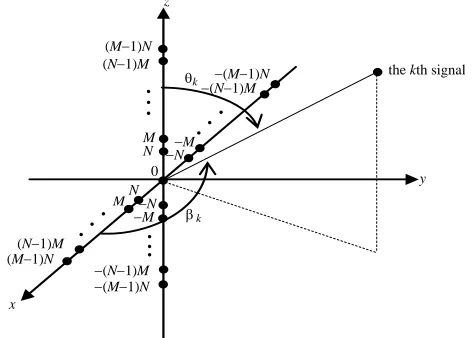
Figure 1 shows the array configuration which comprises two co-prime symmetric linear arrays withX array on x axis, and Z array on z axis. Each sub-array consists of 2(M +N)−3 elements, where M =N+ 1 and M ≥4. The element placed at the origin is common for referencing purpose. The x -coordinate of the elements onXarray and thez-coordinate of the elements onZ array are−(M−1)N d, −(N−1)M d,. . ., 0,. . ., (N −1)M d, (M−1)N d successively, whered≤ λ2. Suppose that there areK narrow band sources impinging on the array. And the sources are uncorrelated with each other. Letθk and βk,k= 1,2, . . . , K, be the elevation angle and azimuth angle of thekth source.
k k N M M −M N −N −N −M (N−1)M
(M−1)N
0
.
.
.
.
.
.
..
.
..
.
β θ z x y−(N−1)M
−(M−1)N
(N−1)M (M−1)N
the kth signal
−(N−1)M
−(M−1)N
Figure 1. Co-prime symmetric sparse cross array configuration.
Let (4N −1)×1 vector x(t) and z(t) be the observed vectors received by X array and Z array respectively, where
x(t) = [x−(M−1)N(t), x−(N−1)M(t), . . . , x0(t), . . . , x(N−1)M(t), x(M−1)N(t)]T
z(t) = [z−(M−1)N(t), z−(N−1)M(t), . . . , z0(t), . . . , z(N−1)M(t), z(M−1)N(t)]T
(1)
Denote θ = [θ1, θ2, . . . , θK], β = [β1, β2, . . . , βK] and 2λdπ = Δ. The received vectors can be
written as
x(t) =A1(β)s(t) +ex(t)
z(t) =A2(θ)s(t) +ez(t) , t= 1,2, . . . , T (2)
where s(t) = [s1(t), s2(t), . . . , sK(t)]T is the non-Gaussian incident signal vector; ex(t) = [ex1(t), . . . , ex(4N−1)(t)]T and ez(t) = [ez1(t), . . . , ez(4N−1)(t)]T are the additive white Gaussian noise with zero-mean at the two sub-arrays; A1(β) = [a1(β1),a1(β2), . . . ,a1(βK)] and A2(θ) = [a2(θ1),a2(θ2), . . . ,a2(θK)] denote the array manifold matrices of X array and Z array;
a1(βk) =
e−jΔ(M−1)Ncosβk e−jΔ(N−1)Mcosβk . . . 1 . . . ejΔ(N−1)Mcosβk ejΔ(M−1)NcosβkT and a2(θk) =
e−jΔ(M−1)Ncosθk e−jΔ(N−1)Mcosθk . . . 1 . . . ejΔ(N−1)Mcosθk ejΔ(M−1)NcosθkT, k =
3. 2-D DOA ESTIMATION USING FOC
3.1. Reconstruction of Cross-Covariance Matrix
In this part, a matrix C∈ C((M+2)N+1))×((M+2)N+1) is constructed in forth-order-cumulants of array received data. And the elements of C can be expressed as Cuv = cum{xa(t), x∗b(t), zc(t), zd∗(t)}. Let (u−1) modN =u1, (u−1)N−u1 =u2, (v−1) modN =v1 and (v−1)N−v1 =v2. Then, we have
u−1 =u1+u2N
v−1 =v1+v2N (3)
where 0≤u1≤N−1, 0≤v1≤N−1, 0≤u2 ≤M+ 2 and 0≤v2 ≤M+ 2.
The element Cuv = cum{xa(t), x∗b(t), zc(t), zd∗(t)} can be obtained as the following rules
⎧ ⎪ ⎪ ⎪ ⎪ ⎪ ⎪ ⎪ ⎨ ⎪ ⎪ ⎪ ⎪ ⎪ ⎪ ⎪ ⎩
a=u1M, b= (u1−u2)N if 0≤u1≤N−1, u2 ≤M−1 a=N(M −1), b=−N ifu1= 0, u2 =M
a=N(M −u1), b=−u1M if 1< u1≤N−1, u2 =M a=N(M −1), b=−2N ifu1= 0, u2 =M+ 1 a=M(N −1), b=−2M ifu1= 1, u2 =M+ 1
a=N(M −u1+ 1), b=−u1M if 2≤u1≤N−1, u2 =M+ 1 a=N(M −1), b=−3N ifu1= 0, u2 =M+ 2
(4) ⎧ ⎪ ⎪ ⎪ ⎪ ⎪ ⎪ ⎪ ⎨ ⎪ ⎪ ⎪ ⎪ ⎪ ⎪ ⎪ ⎩
c=−v1M, d=−(v1−v2)N if 0≤v1 ≤N −1, v2 ≤M−1 c=−N(M −1), d =N ifv1 = 0, v2 =M
c=−N(M −v1), d=v1M if 1< v1 ≤N −1, v2 =M c=−N(M −1), d = 2N ifv1 = 0, v2 =M+ 1 c=−M(N −1), d = 2M ifv1 = 1, v2 =M+ 1
c=−N(M −v1+ 1), d=v1M if 2≤v1 ≤N −1, v2 =M+ 1 c=−N(M −1), d = 3N ifv1 = 0, v2 =M+ 2
(5)
LetC4sk = cum{sk(t), s∗k(t), sk(t), s∗k(t)}, according to (3), (4), (5), we can know that
Cuv= cum{xa(t), x∗b(t), zc(t), zd∗(t)}= K
k=1
C4skejΔ [(u−1) cosβk−(v−1) cosθk] (6)
Denote A¯1 = [¯a1(β1),a¯1(β2), . . . ,a¯1(βK)], A¯2 = [¯a2(θ1),a¯2(θ2), . . . ,a¯2(θK)], C4S = diag(C4s1, . . . , C4sK), where
¯
a1=
1 ejΔ cosβk . . . ej(M+2)NΔ cosβkT (7)
¯
a2=
1 ejΔ cosθk . . . ej(M+2)NΔ cosθkT (8)
From (6), (7), (8), it is easy to know that C = ¯A1C4SA¯H2 , which can be considered as a cross-covariance matrix of the received data from a L-shaped array consisting of two uniform linear arrays. This cross-covariance matrix Ccan be used for many 2D DOA estimation algorithms [9–13]. And the total computation complexity is different for different algorithms. So we only compare the computation complexity of forming cross-covariance matrix for different arrays. For proposed sparse cross array, the resulting multiplications required are in the order ofO((M N+ 2N + 1)2T), where T is snapshots. For the L-shaped array with the same number of elements, the resulting multiplications required are in the order ofO((2M+ 2N−1)2T). Hence, the complexity of forming cross-covariance matrix with proposed cross array is higher than corresponding L-shaped array.
3.2. Improved CESA for 2D DOA Estimation
Similar to CESA presented in method [11], we get the first column of C, and denote it as c1. Then we construct a new vector c
c=
Jc∗1(2 :M N+ 2N+ 1)
c1
wherec1(2 :M N+ 2N+ 1) indicates a column vector consisting of the 2th element to the last element of c1. Using the vector c, we can construct a (2M N+ 4N+ 2−L)×L matrixRc expressed as
Rc = [¯c1 c¯2 . . . ¯cL] (10)
where ¯cl is the column vector consisting of the lth to the (2M N + 4N + 1−L+l)th element of c, M N+ 2N+ 1≥L≥K. Lis a changeable number for counterpoising the computation complexity and precision. We can achieve the estimation of azimuth angles like MUSIC algorithm by maximizing the cost function f(β)
f(β) = 1
aH(β)(I−R
OcRHOc)a(β)
(11)
where, ROcis a (2M N+ 4N+ 2−L)×Lmatrix obtained by the Gram-Schmidt orthogonalization on the column ofRc, and a(β) is a (2M N + 4N + 2−L)×1 vector expressed as
a(β) =1 ejΔ cosβ . . . ej(2M N+4N+1−L)Δ cosβT (12)
Replacing C with CH, we can get the estimation of elevation angles with the same method used for estimating the azimuth angles. Using the corresponding angles matching method [11, 13], we can get the final 2-D DOA estimation.
It should be pointed out that the application of this method has been studied in [11], where authors give the Rc with a fixed number of columns, i.e., the number of sourcesK. In fact, L =K is not the best choice in many conditions. But there is not a strict standard to determine how to choose the best L. Selecting a smallL, the received data can’t be utilized adequately, hence the estimator can’t get high precision and high resolution estimation, especially at low SNR or less snapshots scenarios. But large L will increase the computational burden. In addition, when theLis large enough the improved effect will be not obvious, which can be roughly proved in Experiment 1. Taking an overall consideration, we trend to choice theL slightly larger than the number of signal sources.
Besides of CESA, for the 2D-ESPRIT algorithm with L-shaped proposed in [9, 10], the cross-covariance matrix also is used directly to estimate azimuth angles and elevation angles. Naturally, under the same number of elements, the performance of this algorithm can be improved by exploiting the co-prime symmetric cross array, which can be proved in Experiment 4.
Because of the co-prime symmetric array structure, there is no issue of angle ambiguity need to be concerned [8]. However, a fact we should admit is that the computation complexity will increase when the co-prime symmetric cross array is employed.
4. SIMULATIONS EXPERIMENT
In this section, numerical simulation results are showed to demonstrate the performance of proposed method for 2-D DOA estimation. We consider the geometry structure of the co-prime symmetric cross array as Figure 1, and assume that M = 5, N = 4, d = λ/2. We employ an L-shaped array
consisting of two fifteen-element uniform linear arrays. The number of elements of the cross array is 29 which is equivalent to the L-shaped array. Suppose that the power ratio of signal sources are 1 : 1 in Experiment 1, 2, 3 and 1 : 2 in Experiment 4. The SNR is defended as 10 log10(σ2n
p ), whereσ 2
nrepresents the power of noise and p denotes the average power of all signal sources. The root mean square error (RMSE) is used to be a evaluating index, and it can be expressed as
RMSE =
1
KJ J
j=1 K
k=1
ˆ θkj−θk
2
+ ( ˆβkj−βk)2
(13)
where J = 100 is the number of independent experiments, and ˆθkj, ˆβkj are the estimations of azimuth angle and elevation angle in the jth experiment for the kth signal. For the CESA, the scanning range of the angle is limited within the region of [0◦,90◦] with scanning interval δ = 0.5 in Experiment 1 and δ = 0.1 in Experiment 2, 3. In order to unify the standard, we choose L = 6 for the ICESA in Experiment 2, 3. According to Experiment 1, we can know this selection is reasonable.
(a) (b)
(e) (f)
(c) (d)
4.1. Experiment 1
In the first experiment, we want to compare the performance of ICESA with uniform L-shaped array for different values ofL. The snapshots is fixed 200, SNR is fixed at 5 dB, elevation angles and azimuth angles are fixed at [θ1, θ2] = [40◦,50◦], [β1, β2] = [35◦,45◦] respectively. In this experiment, we also want to find a appropriateLfor the following experiments. Since the elevation angles and azimuth angles are estimated independently in the same method. So, comparing the spatial spectrum of azimuth angles is enough to show the performance of ICESA for different values of L. From Figure 2, we can see that the performance ofL= 6 is very close toL= 8 but better thanL= 2 (CESA), andL= 4. Taking the complexity into account, we chooseL= 6 for Experiment 2, 3.
4.2. Experiment 2
In the second experiment, we compare the angle resolution of CESA with uniform L-shaped array, ICESA with uniform L-shaped array and ICESA with sparse cross array. The snapshots is fixed 200, SNR is fixed at 10 dB, elevation angles and azimuth angles are fixed at [θ1, θ2] = [40◦,50◦], [β1, β2] = [68◦,70◦] respectively. From Figure 3, we can find that the elevation angles with 10◦ interval can be distinguished distinctly by three methods with little difference. For the azimuth angles with 2◦ interval, CESA with uniform L-shaped array can’t distinguish the two angles, and ICESA with uniform L-shaped array can distinguish the two azimuth angles reluctantly. But for ICESA with sparse cross array, the two azimuth angles can be distinguished distinctly. Through the simulation results, we can get the conclusion the angular resolution of ICESA with sparse cross array is the best.
4.3. Experiment 3
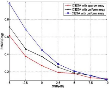
Firstly, we compare the estimation precision of three methods mentioned in Experiment 2 with respect to SNR. Two signal directions are set to [θ1, θ2] = [55◦,65◦], [β1, β2] = [20◦,35◦]. We fix the number of snapshots at 200 with the SNR varying from −5 dB to 10 dB. Secondly, we compare the performance of three methods with respect to the number of snapshots, and two signal directions are set to [θ1, θ2] = [50◦,55◦], [β1, β2] = [45◦,50◦]. The SNR is fixed at 7.5 dB with the number of snapshots changing from 100 to 500. From Figure 4 and Figure 5, we can observe visually that ICESA with sparse cross is better than the other two algorithms, particularly for low SNR. But, we must admit that when SNR is high the accuracy of three methods is very close. Another fact is that the performance of ICESA is more stable with the changes of snapshots.
Figure 4. The estimation RMSE versus SNR (Snapshots = 200).
4.4. Experiment 4
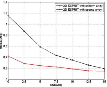
In the fourth experiment, we compare the performance of 2D ESPRIT algorithm with uniform L-shaped array and sparse cross array. Two signal directions are set to [θ1, θ2] = [55◦,65◦], [β1, β2] = [20◦,35◦]. Because of the performance difference between CESA and 2D ESPRIT. The range of SNR in this experiment is different from Experiment 3. Firstly, we fix the number of snapshots at 200 with the SNR varying from 0 dB to 15 dB. Secondly, the SNR is fixed at 10 dB with the number of snapshots changing from 100 to 500. From Figure 6 and Figure 7, we can see that when the co-prime symmetric cross array is used, the performance of 2D ESPRIT will be improved obviously. This experiment again indicates the validity of the co-prime symmetric cross array and the construction method of cross-covariance matrix.
Figure 6. The estimation RMSE versus SNR (Snapshots = 200).
Figure 7. The estimation RMSE versus snapshots (SNR = 10 dB).
5. SUMMARY AND DISCUSSION
In this paper, we present a design approach of co-prime symmetric sparse cross array as well as the construction method of cross-covariance matrix. Simulation results show that the performance of some existing 2-D DOA estimation algorithms can be improved when this special array is exploited. Additionally, an ICESA is also proposed and shows better precision and resolution than that of CESA. The estimation effectiveness can be improved further as the use of the co-prime symmetric cross array. Hence our study can provide a reference for relevant 2-D DOA estimation algorithms.
ACKNOWLEDGMENT
The authors would like to thank the editors and anonymous referees for their comments and suggestions that help us to improve the quality of this paper.
REFERENCES
1. Zhang, X., X. Gao, G. Feng, and D. Xu, “Blind joint DOA and DOD estimation and identifiability results for MIMO radar with different transmit receive array manifolds,”Progress In Electromagnetics Research B, Vol. 18, 101–119, 2009.
2. Albagory, Y. A., “Performance of 2-D DOA estimation for stratospheric platforms communica-tions,” Progress In Electromagnetics Research M, Vol. 36, 109–116, 2014.
4. Vaidyanathan, P. P. and P. Pal, “Sparse sensing with co-prime samplers and arrays,” IEEE Transactions on Signal Processing, Vol. 59, No. 2, 573–586, 2011.
5. Pal, P. and P. P. Vaidyanathan, “Multiple level nested array: An efficient geometry for 2qth order cumulant based array processing,” IEEE Transactions on Signal Processing, Vol. 60, No. 3, 1253– 1269, 2012.
6. Pal, P. and P. P. Vaidyanathan, “Nested arrays: A novel approach to array processing with enhanced degrees of freedom,”IEEE Transactions on Signal Processing, Vol. 58, No. 8, 4167–4181, 2010. 7. Hu, N., Z. F. Ye, X. Xu, and M. Bao, “DOA estimation for sparse array via sparse signal
reconstruction,” IEEE Transactions on Aeronautics and Electronic Systems, Vol. 49, No. 2, 760– 773, 2013.
8. Liang, G. L. and B. Han, “Near-field sources localization based on co-prime symmetric array,” Journal of and Information Technology, Vol. 36, No. 1, 135–139, 2014.
9. Gu, J. F. and P. Wei, “Joint SVD of two cross-correlation matrices to achieve automatic pairing in 2-D angle estimation problems,”IEEE Antennas Wireless Propag. Lett., Vol. 6, 553–556, 2007. 10. Chen, J., S. X. Wang, and X. L Wei, “New method for estimating two-dimensional direction of
arrival based on L-shape array,”Journal of Jilin University (Engineering and Technology), Vol. 1, No. 4, 590–593, 2006.
11. Nie, X. and L. P. Li, “A computationally efficient subspace algorithm for 2-D DOA estimation with L-shaped array,” IEEE Signal Process. Lett., Vol. 21, No. 8, 971–974, 2014.
12. Gan, L., W. F. Lin, X. Y. Luo, and P. Wei, “Estimation 2-D angle of arrival with a cross-correlation matrix,” Journal of the Chinese Institute of Engineers, Vol. 36, No. 5, 667–671, 2013.
13. Kikuchi, S., H. Tsuji, and A. Sano, “Pair-matching method for estimating 2-D angle with a cross-correlation matrix,” IEEE Antennas Wireless Propag. Lett., Vol. 5, 35–40, 2006.