Western University Western University
Scholarship@Western
Scholarship@Western
Electronic Thesis and Dissertation Repository
2-9-2018 10:30 AM
Direct Sheet Molding Compound process (D-SMC)
Direct Sheet Molding Compound process (D-SMC)
Atieh Motaghi
The University of Western Ontario
Supervisor
Dr. Andrew N. Hrymak
The University of Western Ontario
Graduate Program in Chemical and Biochemical Engineering
A thesis submitted in partial fulfillment of the requirements for the degree in Doctor of Philosophy
© Atieh Motaghi 2018
Follow this and additional works at: https://ir.lib.uwo.ca/etd
Part of the Complex Fluids Commons, and the Polymer Science Commons
Recommended Citation Recommended Citation
Motaghi, Atieh, "Direct Sheet Molding Compound process (D-SMC)" (2018). Electronic Thesis and Dissertation Repository. 5284.
https://ir.lib.uwo.ca/etd/5284
This Dissertation/Thesis is brought to you for free and open access by Scholarship@Western. It has been accepted for inclusion in Electronic Thesis and Dissertation Repository by an authorized administrator of
i
Abstract
The combination of highly crosslinked resin and long glass fiber reinforcement in direct sheet
molding compound (D-SMC) provides the parts with high physical properties and low density
suitable for large interior and exterior automotive applications. Different stages of D-SMC process
including maturation zone and compression molding are studied using mathematical analysis,
numerical simulation and experimental investigations.
An analytical analysis is used to calculate the pressure and velocity in the first section of maturation
zone and then the permeability of fiber bundle is calculated by simulation and the agreement
between the available empirical equation and simulation was obtained. The flow is simulated in
the next section of maturation zone using Ansys CFX and it was found the interlocking chain belt
plays an important role in impregnation of bundles with paste.
The microstructure of fiber glass bundles in compression is investigated in a flat plaque mold.
Analyses of the bundle deformation, including bending and deformation of the tow shape, are done
for the charge and specific sites within a square plaque part for 30 percent and 62 percent of initial
charge mold area coverages. Microscopy and micro-computed tomography (micro-CT) of the
samples clarify the microstructure of the bundles after flow. The bundles at the part edge and
corner deform more than the bundles close to center of the mold in both initial charge cases. The
bundles flatten at all positions and bundle bending is mainly observed at the corner. The tow width
changes and tow deflections are higher in the samples of 30 percent mold area coverage. The
micro-CT images show that the bundles keep their cohesion and stay straight within the middle of
the flow path position, but bend at the edge of the mold. Mold filling simulation using MoldflowTM
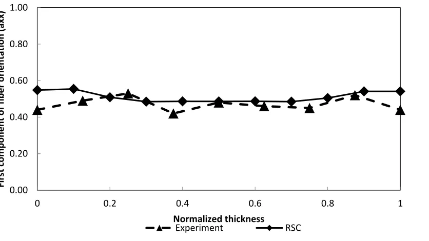
(Autodesk) predict fiber tow orientation through the thickness using the reduced-strain closure
(RSC) models for fiber distribution for 30 and 62 percent initial mold area coverage. The measured
value of orientation from micro-CT images confirms the random orientation through the thickness,
consistent with the RSC model.
The Carreau viscosity model explains the behaviour of the D-SMC paste. Another viscosity model
for suspensions of high volume of planar randomly oriented glass bundles defines the flow
package of OpenFOAM solves the equation of mass and momentum along with the introduced
viscosity model by the volume of fluid technique in the three dimensional system. The simulation
results show the plug flow profile at all positions and times during the process. To study bundle
movement and deformation during the process, it is assumed that regions of very high viscosity
with the same dimension of bundles represent bundles at different positions of the mold. The
results reveal that the bundles close to the edges and corners of the mold moved more than bundles
in the middle and diagonal positions. Moreover, the velocity profile shows higher velocity at these
locations. Experimentally, the red bundles are placed at different locations of the charge and track
during the process. The calculated movement distances of the bundles at different locations from
the experiment and the OpenFOAM simulation follow the same trends and therefore agree.
In D-SMC, there is a viscosity variation through thickness because of temperature gradient and
glass bundle volume fraction variation. The charge is placed between two hot plates of mold which
are then closed to squeeze the charge and filled the mold. The layers of charge close to the hot
mold plates act as lubricant for layers of charge in center. Because of greater resistance of charge
in the center to flow, the hotter lubrication layer may flow preferentially before core layers of
charge. The simulation is run using Ansys Polyflow to study the preferential flow in D-SMC
process. Several stacks of charges on top of each other are used for compression molding. The
flow is simulated for two charges to investigate the evolution of interface during mold filling
Images of cross sections from experimental samples are used to validate the simulation analysis.
Key words
Composite materials, fiber orientation, direct sheet molding compound (D-SMC), numerical
simulation, OpenFOAM, Ansys CFX, Ansys Polyflow, Moldflow, micro computed tomography
Acknowledgements
I would like to thank my supervisor, Dr. Andrew Hrymak, for his unwavering support and
guidance. He encouraged me during every single step of my research, patiently supervised me
during the thesis, gave me freedom to explore new ideas and providing me opportunities for
scientific advancement and personal improvement.
I would like to thank my committee members, Dr. Wankei Wan and Dr. Kibret Mequanint for their
time and advice and the examiners, Dr. Leonardo Simon, Dr. Jeffrey Wood, Dr. Paul Charpentier,
Dr. Amin Rizkalla.
I would like to thank the Fraunhofer Project Center team for helping me producing my samples,
Biotron for microscopy, Robarts research institute-Imaging lab and Center for Automotive
Material (MARC) for micro computed tomography of the samples.
I would like to thank CBE administrative staff, IT help desk people for the welcoming and friendly
environment. I would like to thank my friends in Dr. Hrymak’s research group and my office and
engineering department for all the talks and support and motivation.
My parents are always my role models in my life. Thanks for their constant support and deep love.
Thanks to my sister and brother. Most importantly, I must thank to my husband, Roozbeh, for his
Table of contents
Abstract ... i
Acknowledgements ... iii
List of Tables ... vii
List of Figures ... viii
Nomenclature ... xiii
1 Introduction and literature review ... 1
1.1 Direct sheet molding compound (D-SMC) ... 1
1.2 Formulation ... 4
1.3 Impregnation ... 5
1.4 Compression molding of sheet molding compound ... 6
1.5 Simulation of compression molding of glass fiber filled polyester SMC ... 8
1.6 Rheology of fiber filled suspensions ... 10
1.7 Fiber orientation in polymer processing ... 13
1.7.1 Folgar-Tucker model ... 14
1.7.2 Reduced strain closure (RSC) model ... 15
1.8 Thesis objectives ... 16
1.9 Thesis Outline ... 16
1.10 References ... 17
2 Maturation zone study... 23
2.1 Objective ... 23
2.2 Flow study of material between rolls ... 25
2.2.2 Velocity and pressure profile ... 27
2.3 Permeability ... 29
2.3.1 Image analysis ... 29
2.3.2 Mathematical model of flow into the bundle ... 29
2.3.3 Result of permeability studies ... 31
2.4 Flow study in the maturation zone ... 34
2.4.1 Simulation ... 34
2.4.2 Result of maturation zone simulation ... 34
2.5 Conclusion ... 35
2.6 References ... 35
3 Microstructure Characterization in Direct Sheet Molding Compound ... 37
3.1 Abstract ... 37
3.2 Introduction ... 38
3.3 Material and process ... 39
3.4 Characterization of the microstructure ... 40
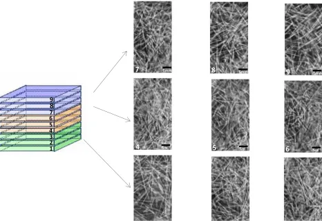
3.4.1 Fiber orientation through the thickness ... 41
3.4.2 In-plane orientation ... 42
3.4.3 Deflection, fiber width and length ... 43
3.4.4 Micro computed tomography ... 44
3.5 Moldflow simulation ... 44
3.6 Result ... 45
3.7 Conclusions ... 57
3.8 References ... 58
4 Simulation of Compression Molding of Direct-Sheet Molding Compound ... 60
4.2 Simulation ... 61
4.2.1 Methodology ... 61
4.2.2 Geometry generation and mesh ... 62
4.2.3 Boundary conditions ... 63
4.2.4 Constitutive equation ... 63
4.3 Results for compression molding ... 66
4.4 Simulation of single bundle deformation in the flow ... 70
4.5 Results for simulation of single bundle ... 73
4.6 Experimental validation ... 73
4.7 Flow patterns in the sheet cross section ... 75
4.8 Conclusion ... 76
4.9 References ... 77
5 Simulation of flow through the thickness direction in DSMC ... 79
5.1 Objective ... 80
5.2 Modelling ... 80
5.2.1 Mathematical modeling ... 80
5.2.2 Constitutive equation ... 81
5.2.3 Boundary condition ... 81
5.2.4 Computational domain and discretization ... 83
5.2.5 Boundary condition ... 84
5.2.6 Finite element algorithm ... 85
5.3 Experimental procedure ... 85
5.3.1 Material and process ... 85
5.3.2 Simulation result ... 86
5.4 Conclusion ... 93
5.5 References ... 94
6 Conclusion and recommendations ... 96
6.1 Conclusions ... 96
6.2 Recommendations for future work ... 97
Appendix A ... 99
Appendix B ... 104
Table 2-1 Parameters used for analysis ... 27
Table 2-2 Bundle properties ... 29
Table 2-3 Permeability values form simulation and equation ... 33
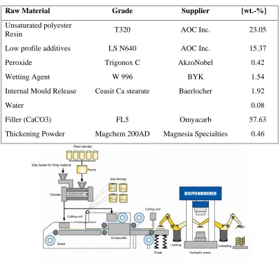
Table 3-1 Formulation of D-SMC paste ... 40
Table 3-2 Parameters for the viscosity model [22] ... 45
Table 3-3 Parameters for the kinetic model [22] ... 45
Table 3-4 Microstructure parameters measured for charge and sheet at for 62 percent initial mold area coverage ... 49
Table 3-5 Microstructure parameters measured for charge and sheet at for 30 percent mold area coverage ... 49
Table 4-1 Formulation of D-SMC paste ... 65
Table 4-2 Parameters of viscosity model ... 66
Table 4-3 Coordinates of points of interest ... 67
Table 5-1 Parameters of viscosity model ... 83
List of Figures
Figure 1-1 Schematic view of D-SMC process [2] ... 3Figure 1-3 Squeeze flow pattern a) shear like flow profile b) plug like flow profile ... 8
Figure 1-4 Steady shear viscosity of SMC of unsaturated polyester versus shear rate for different temperature [38] ... 11
Figure 1-5 Schematic view of the shear deformation of the suspensions [43] ... 12
Figure 2-1 Maturation zone a) deaeration unit b) impregnation unit ... 24
Figure 2-2 Heating and cooling unit ... 24
Figure 2-3 Notation for analysis of flow... 25
Figure 2-4 Pressure profile over the x-direction ... 28
Figure 2-5 Velocity vectors in the analysis region ... 28
Figure 2-6 Simulation domain for bundle ... 30
Figure 2-7 Images of single bundle ... 31
Figure 2-8 Images of cross section of different bundles in the charge ... 32
Figure 2-9 Velocity vs. pressure gradient over viscosity ... 33
Figure 2-10 Geometry of rollers and compound a) compound flow region ... 34
Figure 2-11 Velocity and strain rate in the flow domain ... 35
Figure 3-1 Schematic view of D-SMC process ... 40
Figure 3-2 Positions of samples in the sheet; D: diagonal, M: middle, E: edge, C: corner, positions of the initial charge (30 percent mold area coverage ( – – – – ) , 62 percent mold area coverage (– ‧ – ‧ –) ... 41
Figure 3-4 a) Stitched image of corner sample b) measured parameters of 𝑎𝑖𝑗, 𝑙𝑖, 𝑅𝑖, φ to quantify the fiber bundle. ... 43
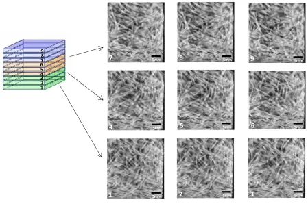
Figure 3-5 Overview of the bundles in charge ... 46
Figure 3-6 Overview of sample cross section ... 47
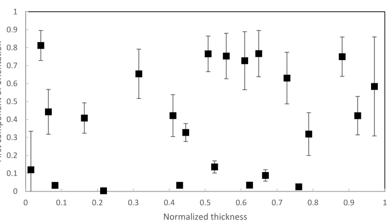
Figure 3-7 First component (x-x) of local fiber bundle orientation through the thickness at position
M, where x and y are the planar directions and z is the thickness direction. ... 47
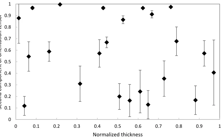
Figure 3-8 Second component (y-y) of local fiber bundle orientation through the thickness at
position M, where x and y are the planar directions and z is the thickness direction. ... 48
Figure 3-9 Micro CT of the E sample for 62 percent of initial mold area coverage (voxel size of
20 𝜇) ... 50
Figure 3-10 Micro CT of the M sample for 62 percent of initial mold area coverage (voxel size of
50 𝜇) ... 51
Figure 3-11 Average cure over time ... 52
Figure 3-12 First component of fiber orientation for sample M of 62 percent of initial mold area
coverage ... 53
Figure 3-13 First component of fiber orientation for sample M of 30 percent of initial mold area
coverage ... 54
Figure 3-14 First component of fiber orientation for sample D of 62 percent of initial mold area
coverage ... 54
Figure 3-15 First component of fiber orientation for sample D of 30 percent of initial mold area
coverage ... 55
Figure 3-16 First component of fiber orientation for sample E of 62 percent of initial mold area
Figure 3-17 First component of fiber orientation for sample E of 30 percent of initial mold area
coverage ... 56
Figure 3-18 First component of fiber orientation for sample C of 62 percent of initial mold area
coverage ... 56
Figure 3-19 First component of fiber orientation for sample C of 30 percent of initial mold area
coverage ... 57
Figure 4-1 Schematic of mold geometry and position of the initial charge ... 62
Figure 4-2 Shear viscosity of D-SMC paste ... 65
Figure 4-3 Points of interest in the sheet; D: diagonal, M: middle, E: edge, C: corner, positions of
the initial charge (30 percent mold area coverage ( — ‧ —) , 62 percent mold area coverage (––
— —), middle line (----) ... 66
Figure 4-4 b) Resulting charge edge at 1.2s from 62 percent mold area coverage, d) resulting charge
edge at 6.8s from 30 percent mold area coverage ... 67
Figure 4-5 Velocity for 62 percent initial mold area at different positions after 1.2 seconds ... 68
Figure 4-6 Velocity profile for 62 percent initial mold area coverage through the thickness at M
and D positions ... 68
Figure 4-7 Velocity profile for 30 percent initial mold area coverage at different positions after 1.2
seconds ... 69
Figure 4-8 Velocity profile for 30 percent initial mold area coverage through the thickness at M
and D positions ... 69
Figure 4-9 Compression molding pressure versus strain rate ... 70
Figure 4-10 Single bundle movement in the mold with 5mm thickness a) initial position b) after
Figure 4-11 Single bundle movement in the mold with 5mm thickness and symmetry boundary
condition a) initial position b) after 1.2s c) velocity (m/s) at 1.2 s ... 72
Figure 4-12 a) Initial positions of bundles b) After 0.5s c) After 1.2 s ... 73
Figure 4-13 Bundle positions a) before compression b) after compression for 62percent mold
coverage ... 74
Figure 4-14 Travel distance of bundles at different locations (cm) ... 75
Figure 4-15 Cross section of the sheet a) two stacks of charges 62 percent initial mold area b) four
stacks of charges 30 percent initial mold area (the flow is from the center of mold (left) to end of
cavity (right)... 76
Figure 5-1 Shear viscosity of paste as a function of shear rate ... 82
Figure 5-2 Shear viscosity of paste including 20 percent GF as a function of shear rate ... 82
Figure 5-3 Finite element mesh of computational domain a) two charges with different viscosities
b) core charge with two layers of paste on top and bottom ... 84
Figure 5-4 Isothermal flow over time for core charge with two layers of paste on top and bottom
... 87
Figure 5-5 Flow and temperature development over time for core charge with two layers of layer
of paste on top and bottom ... 88
Figure 5-6 Isothermal flow development for two layers of charge with paste layer and paste with
GF layer ... 89
Figure 5-7 Temperature and flow development for two layers of charges with paste layer and paste
with GF layer ... 90
Figure 5-8 8 Images of cross section from 30 percent mold area coverage and segmented charge
Figure 5-9 Images of 30 percent initial mold area coverage and layered with two layers of colored
charges on top of two layers of non-colored charges at different positions (1a, 1b, 2a, 2b are images
at the positions of right-hand side sheet) ... 91
Figure 5-10 Images of 30 percent initial mold area coverage and layered with one layer of colored
charge on top of one charge of non-colored charge (4 charges in total) at different positions (1a,
1b, 1c are images at the positions of right-hand side sheet) ... 92
Figure 5-11 Images of 62 percent initial mold area coverage and layered with one non-colored
charge on top of one colored charge at different positions ... 93
Figure 5-12 Microscopy of cross section of charge close to the upper and lower surface ... 93
Nomenclature
𝑎 = minor axis of bundle
𝑎∗ = dimensionless average width of bundle
𝑎𝑖0 = bundle width in the charge
𝑎𝑥𝑥 = component of orientation tensor
𝔸 = forth order orientation tensor
𝐴 = fiber orientation tensor
𝑨 = constant value
𝐴𝑓𝑖𝑏𝑒𝑟 = fiber cross section area
𝐴𝑏𝑢𝑛𝑑𝑙𝑒 = bundle cross section area
𝐴𝑖 = frequency factor
𝑏 = major axis of bundle
𝑩 = constant value
𝑐 = concentration
𝐶𝐼 = fiber-fiber interaction coefficient
𝑐1 = model parameter
𝑐2 = model parameter
𝐶𝑝 = specific heat
𝑑 = fiber diameter
𝐷 = strain rate tensor
𝐸𝑎 = activation energy
𝑓 = distribution function
𝑓𝛼 = interfacial tension force
𝑓𝑐 = contact force
𝑔 = gravity
ℎ = distance between rolls H = heat of reaction
𝑘𝑓 = friction coefficient
𝑘ℎ = hydrodynamic coefficient
𝑘 = thermal conductivity
𝑘𝑝 = penalty coefficient
𝐾 = permeability tensor
𝑙 = fiber length
𝕃 = eingenvectors of orientation tensor
𝑙𝑖 = visible length of bundle
𝕄 = eigenvalues of orientation tensor
𝑚𝛼 = kinetic exponent
𝑛 = parameter of Carreau Bird Model
𝑁𝑓 = number of fibers in the bundle
𝑛𝛼 = kinetic exponent
𝑛1𝛼 = exponent of viscosity model
𝑃 = pressure
𝑃𝑛 = packing stress
𝑄 = flow rate
𝑟 = Radius of fibers
𝑟𝑓 = aspect ratio of fiber
𝑅𝑖 = curvature radius
𝑅 = universal gas constant
𝑡 = time
𝑇 = temperature
𝑇𝑏 = model parameter
𝑻 = stress tensor
𝑢 = velocity vector
𝑢𝑐 = compression velocity
𝑢𝑝𝑙𝑎𝑡𝑒 = velocity of plate
𝑈 = roll speed
𝑣𝑥= velocity in x direction
𝑣𝑦 = velocity in y direction
𝑣𝑓 = volume fraction of fibers in bundle
𝑉𝑓 = Glass bundle volume fraction
W = vorticity tensor
Greek letters
𝛼 = degree of cure
𝛼𝑔 = degree of cure at gelation
𝛼𝑓 = volume fraction of fluid
𝛼𝑎= volume fraction of gas
𝛼𝜂 = average shearing thickness
𝛿∗ = deflection
𝜖 = bundle porosity
𝜂 = viscosity
𝜂∞ = viscosity at shear rate of infinity
𝜂0 = zero shear viscosity
𝜂𝑓 = viscosity of fluid
𝜂𝑎 = viscosity of gas
𝜃∗ = absolute temperature
𝜃𝛼∗ = absolute reference temperature
𝜃 = out of plane angel
𝜄 = dimensionless parameter
κ = paramter of RSC model
𝜆 = parameter of Carreau Bird Model
𝜉 = shape parameter
𝜌 = density
𝜌𝑓 = density of fluid
𝜌𝑎= density of gas
𝜍 = dimensionless parameter
𝜏 = model parameter
𝜑 = in plane orientation angel
1
1
Introduction and literature review
Direct sheet molding compound (D-SMC)
The D-SMC process was developed by the Fraunhofer Institute for Chemical Technology and
commercialized by Dieffenbacher. The process eliminates the several days’ maturation period
required for conventional sheet molding compound (SMC) and reduces cycle time of production.
The continuous nature of the D-SMC process guarantees a high and constant quality of products
compared to the batch process of conventional SMC. In SMC, the preform is wrapped and stored
for certain amount of time for thickening (e.g. 1-2 weeks) before use in compression molding [1].
The time and cost of storing the preforms in the D-SMC process are eliminated. D-SMC offers the
possibility of real time control over the formulation and process. The main stages of D-SMC are
mixing zone, maturation zone and compression molding as shown in Figure 1-1[1].
The process begins with automated dosing of the liquid raw ingredients (e.g. unsaturated
polyester resin, low profile additive, peroxides). All the liquid ingredients are mixed in the twin
screw extruder at room temperature. Solid ingredients (fillers such as calcium carbonate,
thickening and release agent) are added gravimetrically from a side feeder into the extruder. The
extruder mixes the liquid and solid ingredients to form a homogenous paste compound [2].
The paste is divided into two equal streams and transferred into doctor boxes as shown in Figure
1-1. The fiber bundles are cut from rovings and distributed across the width of paste layer. The
sandwich of paste and fiber passes through a roller section for degassing and impregnation of the
resin into the fiber tows, and consistent dispersion where fiber wet out takes place. The
impregnated material then moves through a rapid-maturation zone where, in a
temperature-controlled environment, the chemical thickening of the D-SMC material takes place within a few
minutes. At the end of the maturation zone, the viscosity of mixture increases and then the D-SMC
charge is cooled to ambient temperature. The material moves directly onto the automated
numerically controlled (NC) cutting table, where it is cut into the required charge pattern and
Either manual transfer or a robot picks up the charge and places it in the open tool of a
compression-molding press, which then closes and molds the part. Depending on the sheet width,
throughput and material formulation, the complete cycle — from compounding through molding
— can take as little as 20 minutes[2].
The main features of the D-SMC process are [1, 2];
• Very high efficiency because of lowest possible material costs
• Improved surfaces of the formed parts (class A surface)
• Short cycle time
• Excellent process capability
• Reduced wear on the press dies
• Fewer air inclusions and more homogenous filler dispersion
• No semi finish process
• No semi finish material maturation stage and transportation
• Flexibility in recipe of formulation
• High process stability
The several maturation periods required by SMC is eliminated in D-SMC. With D-SMC the
lengthy interval between compounding raw materials and compression molding can be shortened
to minutes. D-SMC is continuous process compared to the SMC process which is batch process.
Due to close loop nature of D-SMC process, a high and constant level of quality can be guaranteed
that is more challenging in conventional SMC [2].
The scrap in D-SMC process is reduced which has a positive effect on final product costs. Also,
the time and cost of storing material for maturation are eliminated because there is no need to wait
for material to mature. D-SMC provides the greater flexibility in terms of raw material selection
and get close to real time control over formulation changes. The compound consistency is greater
in D-SMC material compared to SMC material because of the twin screw extruder is more
effective than mixers in conventional SMC. D-SMC provides the opportunity to increase the fiber
volume fraction for demanding application. Also, microscopy of D-SMC products shows fewer
air inclusion and finer and more homogenous filler dispersion than conventional SMC products
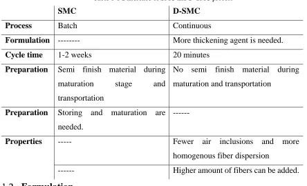
[2]. The main differences of SMC and D-SMC are available in Table 1-1 [1, 2].
Doctor box
Doctor box
Table 1-1 Difference of SMC and D-SMC process
SMC D-SMC
Process Batch Continuous
Formulation --- More thickening agent is needed.
Cycle time 1-2 weeks 20 minutes
Preparation Semi finish material during
maturation stage and
transportation
No semi finish material during
maturation and transportation
Preparation Storing and maturation are
needed.
---
Properties --- Fewer air inclusions and more
homogenous fiber dispersion
--- Higher amount of fibers can be added.
Formulation
The combination of highly crosslinked resin and long glass fiber reinforcement in direct sheet
molding compound (D-SMC) and sheet molding compound (SMC) provides the parts with
improved strength, stiffness, heat resistance and dimensional stability. SMC and D-SMC offer a
great application in automotive industry because of high strength to weight ratio, corrosion
resistance and low cost. Unsaturated polyester (UP) is one of the most commonly used thermoset
resins for SMC and D-SMC. This material has good strength which is required in many demanding
applications [1,3]. Approximately, 75 percent of all resins used for formulation is polyester [3].
The most common type of reinforcement in the SMC and D-SMC industry is glass fibers. They
offer dimensional stability and good mechanical properties. Normally, glass fibers are in the form
of individual bundles and in the range of 25-35 weight percent of SMC/D-SMC. The glass bundles
are randomly distributed in the plane of the sheet. The role of the fillers is necessary for the
improvement of properties such as chemical and heat resistance, dimensional stability, hardness,
surface smoothness and shrinkage. Calcium carbonate is the most common filler in the range of
60-65 weight percent of the paste formulation. Low profile additives (LPA), which are
thermoplastic, control shrinkage during the curing process and provide good surface appearance.
The amount of LPA used in formulations is typically 2-15 weight percent. Thickening agent is
handling the SMC/D-SMC charge and fiber displacement during molding. Too low a viscosity
causes the resin to flow ahead of fibers, and too high a viscosity reduces wet out of the fiber
bundles. Thickening agents include magnesium oxide (MgO), magnesium hydroxide, and calcium
oxide. The thickening agent increases the viscosity up to 105 Pa.s as a result of chain extension by
a condensation reaction between the metal oxides and carboxylic acid groups of unsaturated
polyester. Han et. al. shows that the zero shear viscosity for unsaturated polyester/MgO mixture
increases in thickening period after 450 hour [4]. Other additives such as initiators, mold release,
pigments and stabilizers are also used in SMC formulations [1].
Impregnation
Permeability of fibrous media is a key characteristic of composite manufacturing. The degree of
impregnation of a fiber bundle has a significant influence on the quality and performance of final
product. In SMC and D-SMC, one layer of randomly dispersed chopped fiber bundles is pressed
between two layers of paste.
The permeability of fibrous media is a quality which relates the local velocity of fluid flow to the
pressure gradient. In flow perpendicular to the plane of reinforcement either chopped bundles or
mat as in SMC and RTM, the permeability can be calculated using the Darcy’s law:
〈𝑢〉 = 𝐾
𝜇. 〈∇𝑝〉 (1-1)
In which 𝜇 is viscosity of the fluid, 𝑝 and 𝑢 are the pressure and average velocity of fluid,
respectively. Parameter 𝐾 is permeability tensor of porous medium which has dimension of
𝑚2[5].
It is often impossible to determine the analytical expression for permeability of inter tow region
because of complex path of flow in this region. One of the most popular approaches in numerically
prediction of permeability is solving the Stokes equation and substituting the resulted velocity and
pressure gradient from Stokes equation in Darcy equation [6–11]. Within approach, the
permeability was obtained for woven fabric preform [6], textile [8,11], thermoplastic yarn [9].
Papathanasiou simulated the permeability for the unit cell containing square packing of fibers
inside its perimeter [7,10]. The unit cell was characterized by two porosities: an inter-tow porosity,
fiber arrangement and concentration inside each tow. It was found that with increasing number of
fibers (>37), the intra-tow porosity approached a plateau and consequently the predicted
permeability became independent of the number of fibers. Also, the effect of intra-tow porosity on
permeability was very significant when inter-tow porosity was low (less than 0.4). At high values
of inter-tow porosity the effect was negligible and tow behaved effectively as an impermeable tow
and the fluid preferentially flowed around the bundle [7].
Merhi et al. [12] experimentally showed that at the same volume fraction of bundles, the
permeability is higher for the bundles with lower volume fraction of fibers. Glass mat
thermoplastic (GMT) fabrics exhibit higher permeability than SMC bundles, because bundle in
GMT fabrics orients in flow direction which enhanced permeability. Also permeability follows the
empirical power law model [9,12]. Shih and Lee [13] also measured the permeability of several
glass fiber mats with different fiber architectures. They concluded that the size of the pores outside
the fiber twos and the connections between pores plays and important role in determination of the
permeability of fibrous media.
Gebart [14] developed equations for transverse local permeability of intratow region of both
hexagonal and quadratic arrangement of fibers in tow.
𝐾ℎ𝑒𝑥 = 16 9𝜋√6 [ √ 𝜋 (2√3) ⁄
𝑉𝑓 − 1 ]
5/2
𝑅2
1-2)
𝐾𝑞𝑢𝑎𝑑 = 16 9𝜋√2[√
𝜋 4 ⁄ 𝑉𝑓 − 1]
5/2
𝑅2
1-3)
Where 𝑉𝑓is volume fraction of fibers and can be defined (1 − 𝜖) and 𝜖 is porosity. 𝑅 is the radius
of the fiber, respectively. These equations are widely used to determine the permeability of
intra-tow fibrous media in woven fabrics, aligned fiber, textile reinforcement [6,15,16].
Compression molding of sheet molding compound
The SMC/D-SMC preform or charge typically has a thickness of 2-6 mm with uncured resin. The
cut charge(s) are placed in a hot mold and covers 30 to 70 percent of the mold surface area. The
Complete crosslinking occurs in the mold over time under pressure and heat. Then, the part is
ejected from the open mold and the cycle starts over, as shown in Figure 1-2. When 𝑡 ≤ 𝑡𝑓, the
force increases because of squeezing and heating the charge. At 𝑡𝑓, the charge is pushed to flow
into the cavity and at 𝑡𝑐 the mold filling is finished and compression of the charge happens to
compensate the volume change due to the crosslinking reaction [17].
Figure 1-2 Compression force applied during compression molding [16]
The molding cycle time includes mold filling and curing reaction. The filling time is relatively
short, compared to curing time . The governing parameters in these two regions are different. The
curing reaction is governed by the thermal history, while filling is mainly governed by flow history.
The structural properties of the SMC products are developed through the complete cure of the
resin.
When a material is squeezed between two parallel plates, the pressure drives the material to flow
in the plane of the mold direction [18–20]. Such a flow pattern is similar to compression molding
of SMC and as the plate is moving down, there are gradients of velocity in all directions [18].
Figure 1-3 shows two extreme cases during squeeze flow: shear velocity profile and plug flow
profile. The shear profile is a result of the assumption of no slip at walls. Plug flow occurs when
the material is assumed to completely slip at the walls [20]. The complexity of squeezed flow of
SMC is a result of rheological properties, generation of microstructure, curing of the resin, and
thermal and flow boundary conditions between resin and mold [21].
Co
m
pre
ssi
on fo
Simulation of compression molding of glass fiber filled polyester SMC
All simulations conducted for studying flow in compression molding begin from the governing
equations of motion, continuity and energy. One of the most commonly used models is the
generalized Hele-Shaw model, which describes the flow in compression molding process [3,22–
26]. The boundary conditions for the generalized Hele-Shaw model are as follows: the derivative
of pressure is zero ( 𝜕𝑃
𝜕𝑛= 0) at the mold walls and zero pressure at the freeflow front [22,26]. The
following assumptions are used:
• The thickness of mold is much smaller than the other dimensions. The mold thickness
is changes slowly as a function of x and y.
• The molding compound is incompressible and isotropic.
• The viscosity of the fluid is a function of strain rate, temperature and degree of curing.
Viscoelastic effects and normal stress effects are negligible.
• There is a no slip boundary condition at the surfaces of the mold.
• There is no leakage at the mold edges.
The equations were solved for isothermal Newtonian and power law fluids with the power law
exponent of 0.2 and 0.4. The shape of charge was compared to the experimental data for 30 percent
by weight of GF filled polyester SMC, which was molded isothermally, with good agreement [22].
Barone and Caulk [27] visualized the flow in compression molding by using black and white
layers of SMC (polyester/30 weight percent of GF), and by inserting the white charge within the
black charge (segmented charge). At a closing speed of mold (10mm/s), the layers extend
uniformly with no relative motion between the layers. At a slower closing speed (1.75 mm/s), the
layers close to the mold surface move faster than the core layers. This preferential flow of upper
a mold
mold
Force Force
mold mold
Force Force
b
and lower layers adjacent to the mold surfaces is diminished in thinner charges (3 layers). In the
case of the segmented charge and fast closing speed (10 mm/s), the boundary between the white
and black charges confirm uniform extension and slip at mold surfaces, similar to the layered
experiment. But at the slower closing speed of 1.75 mm/s, preferential flow at the center of charge
is observed, which might be related to pre-mature gelation in the region close to the hot mold
surfaces. Similarly, Odenberger et al. [28] observed the preferential flow of upper and lower layers
for GF filled polyester SMC at a relatively low speed of mold closing (2mm/s) and preferential
flow at the top and bottom layers, which is similar to the observation by Barone and Caulk [27,29]
for high speed closing mold.
Lee et al. [30] simulated the compression by the two dimensional equations of motion,
continuity and energy. Fluid behaviour is assumed to be incompressible and isotropic. The
equations are solved for non-isothermal Newtonian and power law fluid with Arrhenius
dependency on the temperature. The parameters of the Newtonian and power law model are
obtained from fitting the data for polyester charge of SMC and the value of zero shear viscosity
double to approximate the effect of fibers. The result shows that the velocity profile is flat, except
for the thin layer at the mold surface. Because the top layers of charge are in contact with the hot
surface of the mold, the viscosity is reduced resulting in a shear rate profile. The velocity profile
shows the planar extensional deformation. The velocity plot at later time near the end of squeezing
process shows that shear region is thicker as the heat penetrates farther. Also, the velocity profile
is flat and there is a little fountain flow at flow front. The result for thick charge (6 layers) of power
law fluid is similar to the Newtonian fluid except formation of preferential flow near the mold
surfaces.
The phenomenon of fountain flow refers to simple shear flow behind the melt front that is
transferred to the combination of shear and extensional flows as a hot fluid element from the core
area moves toward the mold wall and subsequently solidifies. Mavridis et al. [31] simulated the
fountain flow in compression molding of thermoplastic. The temperature of the mold surfaces is
less than the fluid element, which causes the movement of flow to slow and solidification at the
surface. In molding of thermoplastics vitrification occurs by cooling. The high initial thickness
allows for the variation of flow front velocity which intensifies the fountain effect [31]. But, in the
the preferential flow at the surfaces especially at slow closing speed [27]. Vetrification of SMC
occures by cure reaction which is triggered by high temperature and pressure.
Rheology of fiber filled suspensions
When a suspension of rigid fibers flows in suspending medium, the rheological behavior can
be controlled by either matrix fluid or both coupling matrix fluid and fiber orientation evolution.
The presence of fibers highly affects the rheology, fiber orientation and flow field. In a
homogenous flow field with randomly oriented fibers, all fibers experience the same shear rate as
fluid shear and flow field remains unchanged. In the case of non-homogenous flow and pressure
flow between parallel plates, the fibers near the wall reorient faster because of the higher shear
rate compared to the center line. Therefore, the rheological properties changes and leads to
non-parabolic velocity profile.
The shear and extensional behavior of glass mat thermoplastic (GMT) under compression
molding was examined by Dweib [32]. The shear and extensional viscosities are derived from a
simplified equation of motion with no slip at the wall and power law model for the fluid. Both
shear and extensional viscosities are a function of mold geometry, closing speed, GF content and
power law parameters [32,33]. Thattaiparthasarthy et al. [33] examined the effect of temperature,
fiber length and content on the viscosity of E-glass reinforced polypropylene by using the same
approach of Dweib [32]. It is concluded that the fiber content has a more significant effect on shear
viscosity than any other parameters such as temperature and fiber length for E-glass/PP system.
The effect of fibers on shear viscosity is consistent for thermoplastics and polyester [30,32,33,38].
Thomasset et al. [34] and Ausias et al. [35] proposed the model to describe the shear viscosity
considering the effect of fiber content and orientation. The agreement between prediction and
experiment for polypropylene containing 20 volume percent GF is reasonable. In this approach,
the modeling is based on the dilute suspension in a Newtonian fluid at low shear rate which is far
from the realistic situation [35]. Moreover, the interaction between the fibers is ignored which
plays an important role in the orientation and rheological properties.
Guo et al. [36] modeled the viscosity of low density polyethylene (LDPE) containing a range
of volume fraction of E-GF. Viscosity is the result of contribution of the matrix and fiber. The
at high shear rate. Their result is also consistent with the modeling done by Ramazani et. al [37]
which the fiber matrix interaction have an important effect on shear viscosity of GF reinforced
polydimethyl siloxane. Their model also predicts an increase in shear viscosity with increasing the
amount of GF and fiber-fiber interaction over the whole range of shear rates.
Lee et al. [38] reported that the shear viscosity of polyester paste of SMC charge without GF
could be fitted to the Carreau model (Figure 1-4).
𝜂𝑠− 𝜂∞
𝜂0−𝜂∞ = [1 − (𝜆𝛾̇)
2](𝑛−1)⁄2 (1-4)
𝜂0 and 𝜂∞are the zero shear and infinite viscosities, and 𝜆 is the time constant, and n is the
power law index.
Their results show that zero shear viscosity, 𝜂0, obey Arrhenius relationship. The paste
viscosity, 𝜂, is temperature dependent and follows the Arrhenius equation;
𝜂 = 𝜂0𝑒
[𝛼(𝜃1∗−1
𝜃𝛼∗)] (1-5)
where subscript * represents the absolute temperature scale in Kelvin degree and 𝜂0 is the viscosity
at reference temperature 𝜃𝛼∗ , while 𝛼 is the activation energy [21,38–40]. Lecorre et al. [39] fitted
the viscosity of SMC compound to obtain the activation energy.
Le Corre et al. [39] also reported that compression and shear viscosities follows the power law
behavior for the GF reinforced polyester. Such behavior is reported before the cure reaction started.
Their results indicate that the power law exponent (n) was independent of temperature and GF
content. Similar to the previous research, the same trend of changing viscosities with temperature
and fiber content is observed [32,33]. The shear viscosity is less affected by fiber volume fraction
than compression viscosity, which leads to enhanced anisotropy with increasing fiber content.
Dumont et al. [41] also reported power law relationship for the GF reinforced polyester under
both simple compression and plane compression molding. Interestingly, the same power law
exponent (n=0.44) is reported for plane and simple compression as for shearing [39]. Also, all
viscosities are fitted to the second order polynomial function of fiber volume fractions [41].
Similarly, Abrams et al. [42] obtained the forces during the compression using the power law
model. The power law exponent of 0.43 is reported for 25 volume percent GF low profile SMC.
The assumption of isotropic and power law model is also used by Lee et. al. [30] for simulation of
compression molding of fiber reinforced polyester.
Figure 1-5 Schematic view of the shear deformation of the suspensions [43]
The rheology of the highly planar randomly oriented bundles’ suspensions is a result of interaction
mechanism at bundles contact points. The interaction forces are the sum of friction (𝐹𝑓) and
lubrication (𝐹ℎ) at contact points (Figure 1-5). The proposed model for the viscosity 𝜂 is
𝜂 = 𝑘𝑓𝑃𝑛 𝛾̇ + 𝑘ℎ
16 𝜋2
𝑎
𝑏2𝛼𝑓𝜙𝑏2𝜂0[1 + (𝜆
𝑎 𝛼𝛾̇)
2
]
𝑛−1 2
1-6)
where 𝛾̇ is the shear rate and, 𝑃𝑛 is the normal packing stress. The first term on the right hand side
of the equation represents the frictional force where 𝑘𝑓 is the friction coefficient. The second term
lubrication and 𝛼 is the average shearing thickness of the compound around the contacting bundles.
The constants of 𝜂0, 𝜆 and 𝑛 are Carreau parameters of the paste. 𝜙𝑏 is the volume fraction of
bundles in the compound. The parameter 𝑓 is a distribution function of in-plane bundle orientation,
and its value is 0 for perfect alignment and 2⁄ 𝜋 for in-plane random orientation [43]. The proposed
rheology model includes the yield stress at low shear rate and a power law behavior at high shear
stress. Thomasset et. al also reported a yield stress for shear viscosity of compounds of long fiber
composites [34].
The above model is based on the assumption that the bundles contain a uniform number of fibers,
which are dispersed uniformly in the system. Servais et al. experimentally showed that bundles
deform at lower normal packing stress and have a uniform deformed cross section with the minor
axis, a, and major axis, b. Another assumption is that flow does not affect the fiber cross section
and volume fraction of bundles. The stress direction is perpendicular to the minor axis, and bundles
cannot rotate about their own axis because of the resistance at the available contact points through
the length. Moreover, bundles are square packed and incompressible at the contact points [43].
The comparison of experiments and model shows that equation 1-6) overestimates the viscosities,
which is attributed to the assumptions that ignores the fiber rotation and only sliding of the fibers
is considered [43].
Fiber orientation in polymer processing
Prediction of fiber orientation began with Jeffery’s equation [44]. The proposed equation is for
dilute suspensions in which fibers do not interact with each other.
The fiber suspensions can be divided into three regimes based on the fiber volume concentration
(𝑐) and fiber aspect ratio (𝑙
𝑑).
Dilute regime. In this region, suspension has sufficiently low concentration of fibers so that
fibers can rotate without touching each other. Theoretically, the average distance between fibers
is greater than the length of fiber. The constraint defined for this regime is 𝑐 < (𝑙
𝑑) 2
.
Semi-concentrated regime. In this regime, the rotation of fiber is restricted by other fibers.
The regime is defined by (𝑙
𝑑) 2
< 𝑐 < (𝑙
Concentrated regime. In this regime, the fiber rotation and movement can be severely affected
by fiber-fiber interaction. Glass fiber composites used for industrial applications typically have
fiber concentration in this regime. The constraint defined this regime is 𝑐 > (𝑙
𝑑). 1.7.1 Folgar-Tucker model
Folgar and Tucker developed a model for fiber orientation based on Jeffery’s model. They
introduced a term that takes into account the interaction between fibers [45]. The following are the
assumptions that were made to develop the model for prediction of second order of orientation
tensor (𝑎𝑖𝑗) for high aspect ratio particles:
1. The fibers are rigid cylinders with uniform length and diameter.
2. The fibers are sufficiently large so that Brownian motion is negligible.
3. The center of mass of the particles are randomly distributed.
The equation is written as,
𝐷𝑎𝑖𝑗
𝐷𝑡 = − 1
2(𝑊𝑖𝑘𝑎𝑘𝑗− 𝑎𝑖𝑘𝑊𝑘𝑗) + 1
2𝜉(𝐷𝑖𝑘𝑎𝑘𝑗+ 𝑎𝑖𝑘𝐷𝑘𝑗− 2𝐷𝑘𝑙𝑎𝑖𝑗𝑘𝑙) + 4𝐶𝐼𝛾̇(𝛿𝑖𝑗− 𝛼𝑎𝑖𝑗)
1-7)
With 𝜶 equal to 3 for three-dimensional and 2 for two-dimensional orientation. In equation (1-7),
𝑊𝑖𝑘, 𝐷𝑖𝑘 and 𝐶𝐼 are vorticity, strain rate tensor and fiber-fiber interaction. Parameter of 𝜉 is a shape
parameter and constant and function of particle aspect ratio (𝑟𝑓)
𝜉 =𝑟𝑓
2− 1
𝑟𝑓2+ 1
.
(1-8 )
To approximate the fourth order orientation tensor, 𝑎𝑖𝑗𝑘𝑙, the closure approximation is used to
relate the fourth order orientation tensor to the second order orientation tensor (𝑎𝑖𝑗). The most
commonly used approximations are: linear closure, quadratic closure and the hybrid closure [46–
48]. The most popular one is hybrid and quadratic closure approximation [36,47,49–51].
The experimental result of Folgar and Tucker [40] shows the dependency of 𝐶𝐼 on fiber aspect
𝐶𝐼= 0.0184 𝑒𝑥𝑝 (−0.7148 𝑐 (𝑙
𝑑)). 1-9)
Phan-Thien et al. [48] also fitted a similar empirical model to experimental data.
𝐶𝐼= 𝐴 [1 − 𝑒𝑥𝑝 (−𝐵 𝑐 (
𝑙
𝑑))] 1-10)
The parameters of 𝑨 and 𝑩 are reported as 0.03 and 0.224, respectively [53]. The value of 𝑪𝑰
may range between 0.01-0.0001 [45,52,53].
In simulation of fiber orientation, it is assumed that the flow field is not affected by the fibers
(decoupled approach). The flow field is first obtained for the mold filling process with the
rheological properties of matrix and processing condition [54–56]. Then, equation 1-7 is solved to
obtain the fiber orientation at different mold positions.
The physical meaning of orientation components is related to the principle axis of the fibers. If
the value of 𝑎𝑥𝑥is close to unity, then it means fibers are oriented to the flow direction
(x-direction). The value of 1 indicates the perfect alignment and 0 indicates the fibers are oriented
perpendicular to the flow direction [57]. In the injection molding of fiber reinforced plastics, the
large value of 𝑎𝑥𝑥 near the wall reflects the fact that fibers are aligned to the flow direction and
because of less shear stress at mid plane fiber orientation is not affected by the flow [51,58–60].
1.7.2 Reduced strain closure (RSC) model
Experiments by Sepehr et al. [61] showed that Folgar-tucker model overestimated the fiber
orientation. Later, Wang et al. [62] modified the Folgar-Tucker model to slow down the orientation
and achieve better agreement between experiments and model predictions.
The reduced-strain closure model (RSC) reduces the effect of straining by introducing a scalar
factor, 𝜅. The equation is
DA
Dt = (W. A − A. W) + 𝜉(D. A + A. D − 2[𝔸 + (1 − κ)(𝕃 − 𝕄: 𝔸)]: D) + 2κCI γ̇(I − 3A) (1-11)
where 𝕃 and 𝕄 are functions of the eigenvectors and eigenvalues of the orientation tensor. The 𝛋
Thesis objectives
The overall objective of the research presented in this thesis was to improve the understanding of
different aspects of D-SMC process.
The objectives of this research study are:
1. To determine the pressure and velocity field in maturation zone.
2. To simulate the dependency of permeability to bundle properties by using Ansys CFX
software.
3. To study the microstructure of D-SMC parts using micro computed tomography and
microscopy as well as determine the orientation.
4. To investigate rheology of the paste and compound.
5. To investigate the bundle deformation in the compression molding.
6. To simulate the orientation in compression molding using Moldflow package.
7. To simulate the flow in compression molding by introducing the viscosity for
suspension
of
high volume of planar randomly oriented glass bundles using OpenFOAM package.8. To simulate the flow and heat transfer in compression molding with viscosity variation
through thickness particularly in the interface of charges and upper and lower mold plates.
Thesis Outline
Chapter 1. Introduction and literature review. This chapter represents the background of this
thesis, including D-SMC process, formulation, impregnation and permeability, compression
molding of SMC, simulation of compression molding, orientation models, rheology of fiber filled
compounds and comparison of preferential flow and fountain flow. The objectives of thesis are
provided.
Chapter 2. Maturation zone study. This chapter explores the formation of charge in maturation
zone, investigating the pressure and velocity field and simulation the permeability.
Chapter 3. Microstructure Characterization in Direct Sheet Molding Compound. This chapter
reports the microstructure studies on the D-SMC parts including analysis of the bundle bending
parts, mold filling simulation with prediction of orientation by Moldflow package. This chapter
has been published in Polymer Composites.
Chapter 4. Simulation of Compression Molding of Direct-Sheet Molding Compound. This chapter
presents the simulation of flow by introducing the viscosity model for suspensions of high volume
of planar randomly oriented glass bundles, simulation of bundle movement and experimentally
track the bundle in compression molding.
Chapter 5. Simulation of flow through thickness in D-SMC. This chapter reports the simulation of
flow and heat transfer in compression molding. The behavior of resin rich layer close to the mold
plates and different viscosities of charges are also considered and the main focus is on the interface
of charges and layers close to upper and lower mold plates.
Chapter 6. Concluding remarks. This chapter provides summary contributions and concluding
remarks for this thesis as well as recommendations for future work.
Chapter 7. Appendix. This chapter contains supplementary information for second component of
orientation tensor mentioned in chapter 3.
References
[1] Han CD. Rheology and processing of polymeric materials. 2007.
[2] Malnati P. Formulation flexibility: Direct-SMC.
Http://www.compositesworld.com/articles/formulation-Flexibility-Direct-Smc 2012.
[3] Davis AD, Gramann PJ, Rios AC. compression molding. 2003.
[4] Han CDAE, Lem K. Rheology of Unsaturated Polyester Resins . 11 . Thickening Behavior
of Unsaturated Polyester and Vinyl Ester Resins 1983;28:763–78.
[5] Kaviany M. Principles of Heat Transfer in Porous Media - M. Kaviany - Google Books.
New York: Springer-Verlag; 2012.
[6] Chen Z-R, Lin Ye, Meng Lu. Permeability Predictions for Woven Fabric Preforms. Journal
of Composite Materials 2010;44:1569–86.
[7] Papathanasiou TD. A structure-oriented micromechanical model for viscous flow through
[8] Swery EE, Meier R, Lomov S V, Drechsler K, Kelly P. Predicting permeability based on
flow simulations and textile modelling techniques: Comparison with experimental values
and verification of FlowTex solver using Ansys CFX. Journal of Composite Materials
2016;50:601–15.
[9] Gennaro R, Greco A, Maffezzoli A. Numerical simulation of the microscale impregnation
in commingled thermoplastic composite yarns. Advances in Polymer Technology
2010;29:122–30.
[10] Papathanasiou TD. On the effective permeability of square arrays of permeable fiber tows.
International Journal of Multiphase Flow 1997;23:81–92.
[11] Belov EB, Lomov SV, Verpoest I, Peters T, Roose D, Parnas RS, et al. Modelling of
permeability of textile reinforcements: lattice Boltzmann method. Composites Science and
Technology 2004;64:1069–80.
[12] Merhi D, Michaud V, Kämpfer L, Vuilliomenet P, Månson J-AE. Transverse permeability
of chopped fibre bundle beds. Composites Part A: Applied Science and Manufacturing
2007;38:739–46.
[13] Shih C-H, Lee LJ. Effect of fiber architecture on permeability in liquid composite molding.
Polymer Composites 1998;19:626–39.
[14] Gebart BR. Permeability of Unidirectional Reinforcements for RTM Rproduction. Journal
of Composite Materials 1992;26:1100–33.
[15] Phelan FR, Wise G. Analysis of transverse flow in aligned fibrous porous media.
Composites Part A: Applied Science and Manufacturing 1996;27:25–34.
[16] Wong CC, Long AC, Sherburn M, Robitaille F, Harrison P, Rudd CD. Comparisons of
novel and efficient approaches for permeability prediction based on the fabric architecture.
Composites Part A: Applied Science and Manufacturing 2006;37:847–57.
[17] Tadmore Z, Gogos CG. Principles of polymer processing. 2006.
[18] Macoskow CW. Rheology Principles, measurments and applications. 1994.
A review. Journal of Non-Newtonian Fluid Mechanics 2005;132:1–27.
[20] Servais C, Luciani A, Månson J-AE. Squeeze flow of concentrated long fibre suspensions:
experiments and model. Journal of Non-Newtonian Fluid Mechanics 2002;104:165–84.
[21] Dumont P, Orgéas L, Favier D, Pizette P, Venet C. Compression moulding of SMC: In situ
experiments, modelling and simulation. Composites Part A: Applied Science and
Manufacturing 2007;38:353–68.
[22] Lee C-C, Folgar F, Tucker CL. Simulation of Compression Molding for Fiber-Reinforced
Thermosetting Polymers. Journal of Engineering for Industry 1984;106:114.
[23] Osswald TA. General results on the flow of chopped fiber compounds in compression
molding 1987.
[24] Advani SG, Tucker CL. A numerical simulation of short fiber orientation in compression
molding. Polymer Composites 1990;11:164–73.
[25] Tucker CL, Folgar F. A model of compression mold filling. Polymer Engineering and
Science 1983;23:69–73.
[26] Park CH, Lee WI, Yoo YE, Kim EG. A study on fiber orientation in the compression
molding of fiber reinforced polymer composite material. Journal of Materials Processing
Technology 2001;111:233–9.
[27] Barone MR, Caulk DA. Kinematics of flow in sheet molding compounds. Polymer
Composites 1985;6:105–9.
[28] Odenberger PT, Andersson HM, Lundström TS. Experimental flow-front visualisation in
compression moulding of SMC. Composites Part A: Applied Science and Manufacturing
2004;35:1125–34.
[29] Barone MR, Caulk DA. A Model for the Flow of a Chopped Fiber Reinforced Polymer
Compound in Compression Molding. Journal of Applied Mechanics 1986;53:361.
[30] Lee C-C, Tucker CL. Flow and heat transfer in compression mold filling. Journal of
Non-Newtonian Fluid Mechanics 1987;24:245–64.
in the compression of polypropylene disks: Experiments and simulation. Journal of
Rheology 1992;36:27.
[32] Dweib MA, Brdaigh CM. Compression molding of glass reinforced thermoplastics:
Modeling and experiments. Polymer Composites 2000;21:832–45.
[33] Thattaiparthasarthy KB, Pillay S, Vaidya UK. Rheological characterization of long fiber
thermoplastics – Effect of temperature, fiber length and weight fraction. Composites Part
A: Applied Science and Manufacturing 2009;40:1515–23.
[34] Thomasset J, Carreau PJ, Sanschagrin B, Ausias G. Rheological properties of long glass
fiber filled polypropylene. Journal of Non-Newtonian Fluid Mechanics 2005;125:25–34.
[35] Ausias G, Agassant JF, Vincent M, Lafleur PG, Lavoie PA. Rheology of short glass fiber
reinforced polypropylene. Journal of Rheology 1992;36:525.
[36] Guo R, Azaiez J, Bellehumeur C. Rheology of fiber filled polymer melts: Role of
fiber-fiber interactions and polymer-fiber-fiber coupling. Polymer Engineering & Science
2005;45:385–99.
[37] Ramazani a., Ait-Kadi a., Grmela M. Rheological modelling of short fiber thermoplastic
composites. Journal of Non-Newtonian Fluid Mechanics 1997;73:241–60.
[38] Lee LJ, Marker LF, Griffith RM. The rheology and mold flow of polyester sheet molding
compound. Polymer Composites 1981;2:209–18.
[39] Lecorre S, Orgeas L, Favier D, Tourabi A, Maazouz A, Venet C. Shear and compression
behaviour of sheet moulding compounds. Composites Science and Technology
2002;62:571–7.
[40] Kenny JM, Opalicki M. Processing of short fibre/thermosetting matrix composites.
Composites Part A: Applied Science and Manufacturing 1996;27:229–40.
[41] Corre S Le, Favier D, Dumont P, Orge L. Anisotropic viscous behavior of sheet molding
compounds ( SMC ) during compression molding 2003;19:625–46.
[42] Abrams LM, Castro JM. Predicting molding forces during sheet molding compound (SMC)
[43] Servais C, Luciani A, Månson J-AE. Fiber–fiber interaction in concentrated suspensions:
Dispersed fiber bundles. Journal of Rheology 1999;43:1005.
[44] Jeffery GB. The Motion of Ellipsoidal Particles Immersed in a Viscous Fluid. Proceedings
of the Royal Society A: Mathematical, Physical and Engineering Sciences 1922;102:161–
79.
[45] Folgar F, Tucker CL. Orientation Behavior of Fibers in Concentrated Suspensions. Journal
of Reinforced Plastics and Composites 1984;3:98–119.
[46] Advani SG. Closure approximations for three-dimensional structure tensors. Journal of
Rheology 1990;34:367.
[47] Kagarise C, Miyazono K, Mahboob M, Koelling KW, Bechtel SE. A constitutive model
for characterization of shear and extensional rheology and flow induced orientation of
carbon nanofiber/polystyrene melt composites. Journal of Rheology 2011;55:781.
[48] Advani SG, Tucker CL. The Use of Tensors to Describe and Predict Fiber Orientation in
Short Fiber Composites. Journal of Rheology 1987;31:751–84.
[49] Kagarise C, Xu J, Wang Y, Mahboob M, Koelling KW, Bechtel SE. Transient shear
rheology of carbon nanofiber/polystyrene melt composites. Journal of Non-Newtonian
Fluid Mechanics 2010;165:98–109.
[50] Wang Y, Xu J, Bechtel SE, Koelling KW. Melt shear rheology of carbon
nanofiber/polystyrene composites. Rheologica Acta 2006;45:919–41.
[51] Oumer AN, Ali AMS, Mamat OB. Numerical Simulation of Fibre Orientation in Simple
Injection Molding Processes n.d.
[52] Bay RS. Fiber orientation in injection-molded composites : A comparison of theory and
experiment. PhD thesis, University of Illinois at Urbana-Chamaign, 1991.
[53] Phan-thien N, Fan X, Tanner RI, Zheng R. Folgar – Tucker constant for a fibre suspension
in a Newtonian fluid 2006;103:251–60.
[54] Vincent M, Giroud T, Clarke A, Eberhardt C. Description and modeling of fiber orientation
[55] Jackson WC, Advani SG, Tucker CL. Predicting the Orientation of Short Fibers in Thin
Compression Moldings. Journal of Composite Materials 1986;20:539–57.
[56] Bay RS, Tucker CL. Fiber orientation in simple injection moldings. Part I: Theory and
numerical methods. Polymer Composites 1992;13:317–31.
[57] Miled H, Silva L, Agassant J, Coupez T. Numerical Simulation of Fiber Orientation and
Resulting Thermo-Elastic Behavior in Reinforced Thermo-Plastics. Mechanical Response
of … 2008;10:293–313.
[58] Oumer AN, Mamat O. A study of fiber orientation in short fiber-reinforced composites
with simultaneous mold filling and phase change effects. Composites Part B: Engineering
2012;43:1087–94.
[59] Vincent M, Devilers E, Agassant J-F. Fibre orientation calculation in injection moulding
of reinforced thermoplastics. Journal of Non-Newtonian Fluid Mechanics 1997;73:317–26.
[60] Miled H, Silva L, Coupez T, Agassant JF. Injection Molding of Fibre Reinforced
Thermoplastics: Integration of Fibre Orientation and Mechanical Properties Computations.
International Polymer Processing 2012;27:547–56.
[61] Sepehr M, Ausias G, Carreau PJ. Rheological properties of short fiber filled polypropylene
in transient shear flow. Journal of Non-Newtonian Fluid Mechanics 2004;123:19–32.
[62] Wang J, O’Gara JF, Tucker CL. An objective model for slow orientation kinetics in
concentrated fiber suspensions: Theory and rheological evidence. Journal of Rheology
2
Maturation zone study
Objective
The maturation process includes a continuous forming operation with pairs of rolls that form a
mass of paste material and distributed fiber bundles into a charge. The paste in the doctor boxes is
spread over the foil, with an adjustable thickness, and the glass bundles are distributed on top of
and over the width of paste. Then, a top layer of paste foil covers the glass bundles (Figure 2-1).
As shown in Figure 2-1a, the rolls squeeze the foils together with paste and glass bundles at room
temperature. At this stage, the air caught in the spreading process is evacuated via the edge area of
the foil. The sandwich of paste and bundles passes through the rollers to smoothly deaerate and
impregnate the bundles. The foil is transported to impregnation zone to ensure the impregnation
of the fiber bundles with paste at room temperature (Figure 2-1b). The rolls move the charge to
the heating zone with controlled temperature. The temperature is set depends on the formulation
of the paste. The charge is heated by the heating plates in the first and second level. As shown in
Figure 2-2, the charge moves in this section while spending enough time for the paste to thicken
and gain enough strength and resistance for handling and compression. At last stage of this section,
the charge is cooled down to the ambient temperature. The full line of maturation zone provides
the optimum impregnation, good binding of the resin onto the bundles and elevated viscosity of
the paste in short period. All these parameters are required for the compression molding of
application with improved mechanical properties.
When a sandwich of paste and bundles are squeezed in the first section (Figure 2-1a), the flow is
laminar into and in between the fiber bundles. By simplifying assumptions, it is possible to make
a mathematical analysis of the operation. Having the physical properties of materials, the
dimensions of rolls, the speed and gap distance, the velocity field and pressure is calculated in this
section.
In the next part, permeability for flow transverse to a unidirectional bundle is investigated. The
When the charge passes through the maturation zone between rolls (Figure 2-1b), the flow is
modeled to learn more about this section of the process.
Figure 2-2 Heating and cooling unit
a b
![Figure 1-1 Schematic view of D-SMC process [2]](https://thumb-us.123doks.com/thumbv2/123dok_us/1936363.1254400/22.612.72.468.72.277/figure-schematic-view-d-smc-process.webp)
![Figure 1-4 Steady shear viscosity of SMC of unsaturated polyester versus shear rate for different temperature [38]](https://thumb-us.123doks.com/thumbv2/123dok_us/1936363.1254400/30.612.209.416.448.689/figure-steady-viscosity-unsaturated-polyester-versus-different-temperature.webp)