EYAL Z. GOREN & KRISTIN E. LAUTER
1. Introduction
While the main goal of this paper is to give a bound on the denominators of Igusa class poly-nomials of genus 2 curves, our motivation is two-fold: on the one hand we are interested in applications to cryptography via the use of genus 2 curves with a prescribed number of points, and on the other hand, we are interested in construction of class invariants with a view towards explicit class field theory and Stark’s conjectures. In the following we give an overview of these motivating problems and explain the contents of the paper.
Some basic protocols in public key cryptography such as key exchange and digital signatures rely on the assumption that the discrete logarithm problem in an underlying group is hard. Current available alternatives favor the use of the group of points on an elliptic curve or the Jacobian of a hyperelliptic genus 2 curve over a finite field as the underlying group. The security of the system depends on the largest prime factor of the group order, so it is crucial to be able to construct curves such that the resulting group order is prime. Also, for applications in pairing-based cryptography, it may be necessary to impose additional divisibility conditions on the group order. Parameterized families of curves satisfying these type of conditions are called pairing friendly curves. Thus algorithms to construct curves with prescribed group orders are required. Currently, typical minimum security requirements require a group size of at least 2256 when the
best-known attacks are square-root algorithms, giving roughly 128 bits of security. Compared to elliptic curves, Jacobians of genus 2 curves are an attractive alternative because they offer comparable security levels over a field of half the bit size, since the group size of the Jacobian of a genus 2 curve over a finite field Fp is roughly p2, whereas elliptic curves have group size
roughly p.
In the case of elliptic curves, the polynomial-time point-counting algorithm proposed by Schoof and improved by Elkies and Atkin (or the newer Arithmetic-Geometric mean algorithm) allows the following approach: one can pick elliptic curves over a finite field of cryptographic size and count points until a prime group order is found. This solution will not work for generating pairing-friendly curves however. Also, over prime fields of cryptographic size, it will not work for hyperelliptic curves of genus greater than one, either. Starting with the work of Atkin and Morain on generating elliptic curves with a prescribed group order for primality proving, the standard approach to constructing such curves has been to use the theory of Complex Multiplication in the so-called CM method.
Given a prime number p, and a non-negative group order N lying in the Hasse-Weil interval [p+ 1−2√p, p+ 1 + 2√p], the goal is to produce an elliptic curve E overFp withN Fp-points:
#E(Fp) =N =p+ 1−t, wheretis the trace of the Frobenius endomorphism of E overFp. Set
D=t2−4p. The Frobenius endomorphism of E has characteristic polynomialx2−tx+p, so it
1991Mathematics Subject Classification. Primary 11G15, 11G16 Secondary 11G18, 11R27.
follows from the quadratic formula that the roots of this polynomial lie inQ(
√
D). It is standard to associate the Frobenius endomorphism with a root of this polynomial. IfEis not supersingular, thenR, the endomorphism ring ofE, is an order in the ring of integers ofK=Q(
√
D). Now the problem is transformed into one of generating elliptic curves with endomorphism ring equal to an order in K. The correspondance between isomorphism classes of elliptic curves overQ with
endomorphism ring equal to OK and primitive, reduced, positive definite binary quadratic forms
of discriminant D gives an easy way to run through all such elliptic curves.
Define the Hilbert class polynomialHD(X) associated to the fieldK as follows:
HD(X) =
Y
X−j −b+ √
D 2a
!!
,
where the product ranges over the set of (a, b) ∈ Z2 such that ax2+bxy +cy2 is a primitive,
reduced, positive definite binary quadratic form of discriminant Dfor somec∈Z, andj denotes the modular j-function. The degree of HD(X) is equal to hK, the class number of K, and it is
known that HD(X) has integer coefficients. To find an elliptic curve modulo p with N points
over Fp, it suffices to find a root j of HD(X) modulo p. One can then reconstruct the elliptic
curve from its j-invariant j. Assuming j 6= 0,1728 and p 6= 2,3, the required elliptic curve is given by the Weierstrass equation y2=x3+ 3kx+ 2k, where k= 1728j−j. The number of points on the elliptic curve is either p+ 1−t orp+ 1 +t, and one can easily check which one it is by randomly picking points and checking whether they are killed by the group order.
There are at least three approaches to computing the Hilbert class polynomial. The complex analytic approach computes HD(X) as an integral polynomial by listing all the relevant binary
quadratic forms, evaluating thej-function as a floating point integer with sufficient precision, and then taking the product and rounding the coefficients to nearest integers. The Chinese remainder theorem (CRT) approach computes HD(X) mod`for sufficiently many small primes`and then
uses the Chinese remainder theorem (CRT) to compute HD(X) as a polynomial with integer
coefficients. The p-adic approach uses p-adic lifting to approximate the roots and recognize the polynomial. These algorithms are all satisfactory in practice for small D, and the current world record for the largestDfor whichHD(X) has been computed is held by the Explicit CRT method
for some|D|>1013 [Sut].
The situation for generating genus 2 curves is more difficult. The moduli space of genus 2 curves is 3-dimensional and so at least 3 invariants are needed to specify a curve up to isomorphism, and, in fact, Igusa’s results show that most genus curves are determined by 3 invariants. The CM algorithm for genus 2 is analogous to the Atkin-Morain CM algorithm for elliptic curves just described. But whereas the Atkin-Morain algorithm computes the Hilbert class polynomial of an imaginary quadratic fieldK by evaluating the modularj-invariants of all elliptic curves with CM by K, the genus 2 algorithm computes Igusa class polynomials of a quartic CM field K by evaluating the modular invariants of all the abelian varieties of dimension 2 with CM by K.
For a primitive quartic CM field K we can define Igusa class polynomials hi(X) =
Y
τ
(X−ji(τ)), i= 1,2,3,
curve associated to the CM point. Note that thej-invariant of an elliptic curve can be calculated in two ways, either as the value of a modular function on a lattice defining the elliptic curve as a complex torus over C, or directly from the coefficients of the equation defining the elliptic
curve. Similarly for genus 2 curves, the triple of Igusa invariants of a genus 2 curve can also be calculated in two different ways. Using classical invariant theory over a field of characteristic zero, Clebsch defined the triple of invariants of a binary sextic f defining a genus 2 curve y2 =f(x). Bolza showed how those invariants could also be expressed in terms of theta functions on the period matrix associated to the Jacobian variety and its canonical polarization over C. Igusa
showed how these invariants could be extended to work in arbitrary characteristic, and so the invariants are often referred to as Igusa or Clebsch-Bolza-Igusa invariants. These invariants will be discussed in more detail in § 2 below. To recover the equation of a genus 2 curve given its invariants, Mestre gave an algorithm which works in most cases, and involves possibly passing to an extension of the field of definition of the invariants ([Mes]).
The CM algorithm for genus 2 curves takes as input a quartic CM field K and outputs the Igusa class polynomials with coefficients in Q and if desired, a suitable prime p and a genus 2
curve over Fp whose Jacobian has CM by K. The CM algorithm was first implemented by
Spallek [Spa], van Wamelen [Wam], and Weng [Wen]. Alternative algorithms for computing Igusa class polynomials have also been proposed and studied, such as the genus 2 Explicit CRT algorithm [EL] and a p-adic approach [GHKRW].
To compute the Igusa polynomials, Spallek [Spa] determined a collection of period matrices which form a set of representatives for isomorphism classes of polarized abelian surfaces with CM by a given field. Determining this set was complicated, and a complete set of representatives in general was not determined until the recent work of Streng [Str]. In [Wen], Weng gave an algorithm for computing the minimal polynomials of Igusa invariants by evaluating Siegel modular forms to very high precision in order to recognize the coefficients of the minimal polynomials as rational numbers. Unfortunately, the polynomials hi(X) have rational coefficients, not integral
coefficients, which makes them harder to recognize from floating point approximations. The large number of floating point multiplications performed in the computation causes loss of precision and makes the algorithm hard to analyze. The running time of the CM algorithm had until recently not yet been analyzed due to the fact that no bound on the denominators of the coefficients of the Igusa class polynomials was known.
Since the polynomialshi(X) have rational coefficients, we can ask about the prime factorization
the corresponding CM cycle, was studied and a precise conjecture was formulated. In subsequent work of Yang, the conjecture was proved for certain classes of quartic CM fields, thereby giving tight bounds on the size of the denominators in those cases. But a general bound needed for the complexity analysis has not been known until the work of the present paper.
The investigations carried out in this paper also have a completely different motivation, which comes from class field theory and Stark’s conjecture. Consider the modular form that we call Θ in this paper (§2.4); it is the unique Siegel cusp form of weight 10 and full level, up to a scalar, and is equal, up to a scalar, to the product of the squares of the 10 even Riemann theta functions of integer characteristics. In many ways Θ is the analogue the elliptic cusp form ∆ of weight 12. Because of this analogy, Goren and Deshalit have studied in [DSG] certain algebraic numbers constructed from values of Θ at CM points associated to a primitive quartic CM field K, whose definition parallels the definition of the Siegel units. Certain expressions in such values gave quantities u(a,b) associated to certain ideals inK, that depend also on the choice of CM type. These quantities lie in the Hilbert class field of the reflex field of K and have many appealing properties, such as a nice transformation law under Galois automorphism, and their dependence only on the ideal classes of a andb. Thus, one is justified in calling them class invariants.
A natural question that arose is whether these invariants are actually units, or close to being units, in the sense that one knows their exact prime factorization, and these primes are small relative to, say, the discriminant of the fieldK. While we do not have complete solutions, several results concerning these have been obtained by the authors in recent years [GL1, GL2]. See also [Val] for numerical data. One of the main reasons to study such quantities is Stark’s conjecture. Recall that for a number field K and m, a modulus in K divisible by all the infinite primes, Stark’s conjecture asserts that if ζ(K;A,0) = 0 then there exists a unit u(A) of K[m] (the associated ring class field) such that
ζ0(K,A,0) = log|u(A)|,
where ζ(K;A, s) is the partial zeta function associated to an ideal class A modulo m. In spite of much work in this area, it is fair to say that Stark’s conjecture is essentially completely open. It is believed that the main obstacle is finding a “good” construction of units, and that was precisely the motivation of [DSG], although the problem of relating the class invariants u(a,b) toL-functions is still outstanding.
Now, as it turns out, the denominators occurring in the coefficients of the Igusa class polyno-mials hi have to do with the modular form Θ as well, and essentially both questions - the nature
of the denominators and the factorization of the invariantsu(a,b) - have the same underlying geo-metric question, which is whether an abelian surface with CM byK, over some artinian local ring, can be isomorphic to a product of elliptic curves (with additional conditions on polarizations). The main theorem of the paper is the following.
Theorem 7.0.4. Let f =g/∆k be a modular function of level one onH2 where:
(1) ∆ is Igusa’sχ10, the product of the squares of the ten Riemann theta functions with even integral chracteristics, normalized to have Fourier coefficients that are integers and of g.c.d. 1.
Then f(τ)∈L=N HK∗ and
(1.0.1) valpL(f(τ))≥
−4kelogp
dTr(r)2 2
+ 1
e≤p−1 −4ke8 logpdTr(r)2 2+ 2 any other case.
Furthermore, unless we are in the situation of superspecial reduction, namely, we have a check mark in the last column of the tables in §3, valpL(f(τ))≥0. The valuation is normalized so that a uniformizer at pL has valuation 1.
Corollaries 7.1.1, 7.1.3, of this theorem give the applications to denominators of Igusa class polynomials and class invariants described above.
In order to prove this theorem, we develop several tools that are of independent interest. The first one is an explicit determination of the reduction of abelian surfaces with complex multiplication. The main invariants of an abelian surface A over a field of characteristic p > 0 are its f-number, that determines the size of the ´etale quotient ofA[p], and the a-number that determines the size of the local-local part of that group scheme. These numbers determine, for example, in which Ekedahl-Oort strata the moduli point corresponding to A lies. It turns out, and that was essentially known by [Gor] and [Yu], that these numbers can be read from the prime factorization ofp in the normal closureN ofK overQand the CM type. However, to our
knowledge, a complete analysis had not appeared in the literature, and we make this analysis explicit here, dealing also with ramified primes, in a self-contained manner.
For a primepto appear in the denominators of thehi, or forp|pto appear in the factorization
of au(a,b), some abelian surface with CM byKmust be isomorphic overFpto the product of two
supersingular elliptic curves E×E0. This givesf = 0, a= 2, and so sieves out the “evil primes” according to their factorization in N. A further, and most important condition, is imposed by the fact that the Rosati involution of E ×E0 must induce complex conjugation on K. We are able to translate the fact that a prime appears to a certain power in the denominators of the hi
(similarly for theu(a,b)) to the fact that a similar situation must hold over a certain artinian ring (R,m) and the index of nilpotency ofmis proportional to the power of the prime. This requires some results in intersection theory (§5) and the introduction of an auxiliary moduli space (§4).
A certain maneuver, already used in [GL1], allows us to reduce the problem to a question about endomorphisms of elliptic curves overRwhose reduction modulomis supersingular. Some special instance of this problem was studied by Gross in [Grs], but his results do not suffice for our purposes. We approach this problem using crystalline deformation theory in§6; in the course of developing the results we need, we provide some more general results that are natural in that context and will, so we believe, be useful for others. Since crystalline deformation theory is only valid under certain restrictions on ramification, we provide an alternative approach that works without any restriction (§6.6) and gives results that are not too much worse than crystalline deformation theory gives.
2. Moduli of curves of genus 2
2.1. Curves of genus two - Igusa’s results. Let y1, y2, y3 be independent variables and let
[ζ](yi) := ζiyi (and trivially on the coefficients). The ring of invariants is defined over Zand we
denote it, by abuse of notation,
Z[y1, y2, y3, y4]µ5.
One of Igusa’s main results [Igu1, p. 613] is thatM2, the coarse moduli space of curves of genus 2,
satisfies
(2.1.1) M2∼= Spec(Z[y1, y2, y3, y4]µ5).
This ring of invariant elements is generated over Z by 10 elements. We remark that outside the
prime 2, namely if we work over Z[1/2], we can dispense withy4 and conclude that
M2⊗Z[1/2]∼= Spec(Z[1/2][y1, y2, y3]µ5).
(Same abuse of notation.) Note that to find generators overZ[1/2] forZ[1/2][y1, y2, y3]µ5 amounts
to finding vectors (a, b, c)∈Z3≥0 such thata+ 2b+ 3c≡0 (mod 5) that generate the semigroup
{(a, b, c) ∈ Z3
≥0 :a+ 2b+ 3c ≡ 0 (mod 5)} – one associate to the vector (a, b, c) the monomial
y1ay2byc3. Such generators are given by the following 8 triples:
(2.1.2) {(0,0,5),(0,5,0),(5,0,0),(0,1,1),(1,2,0),(3,1,0),(1,0,3),(2,0,1)}.
On the other hand, given a field k of odd characteristic, to find generators for the fraction field Frac(k[y1, y2, y3]µ5), one needs generators for the group {(a, b, c) ∈ Z3 : a+ 2b+ 3c ≡ 0
(mod 5)}, which one can choose to be the vectors (2,−1,0),(3,0,−1),(5,0,0) (corresponding to the monomialsy12/y2, y31/y3, y15), for example.
Igusa’s construction is based on much earlier work by Clebsch and others on invariants of sextics. A genus 2 curve is hyperelliptic, where a hyperelliptic curve is defined to be a curve which is a double cover of the projective plane. In characteristic different from 2 the situation is very much like over the complex numbers, and one can conclude that such a curve can be written as y2 = f(x), where f(x) is a separable monic polynomial of degree 6, uniquely determined up to projective substitutions, thus reducing the problems of classifying genus 2 curves to studying when two sextics are equivalent under a projective transformation, or, equivalently, studying the space parameterizing unordered 6-tuples of points in P1.
2.2. Igusa’s coordinates. To describe the invariants of sextics we use Igusa’s notation. Let y2 =f(x) =u0x6+u1x5+· · ·+u6,
be a hyperelliptic curve and let x1, . . . , x6 be the roots of the polynomial f(x). The noation (ij)
is a shorthand for the expression (xi−xj). Consider then
A(u) = u20 X
fifteen
(12)2(34)2(56)2 (2.2.1)
B(u) = u40X
ten
(12)2(23)2(31)2(45)2(56)2(64)2 (2.2.2)
C(u) = u60X
sixty
(12)2(23)2(31)2(45)2(56)2(64)2(14)2(25)2(36)2 (2.2.3)
D(u) = u100 Y
i<j
(ij)2 (2.2.4)
objects into two groups and then finding a matching between these two groups: there are 10 ways to partition into 2 groups and six matching between the two chosen groups. The invariants A, B, C, D are denoted A0, B0, C0, D0 in [Mes, p. 319], but we follow Igusa’s notation; these invariants are often called now theIgusa-Clebsch invariants. Another common notation one finds in the literature is I2 = A, I4 = B, I6 = C, I10 = D, for example in the Magma help pages on
February 2010, but we shall avoid using it, especially since it conflicts with Igusa notation as in [Igu4, p. 848].
The invariants A, B, C, D are homogenous polynomials of weights 2,4,6 and 10, respectively, in u0, . . . , u6, thought of as variables. In addition they are invariants of index 6,12,18 and 30,
respectively. This means the following: Let f(x, z) be the homogenized form of f, that is, f(x, z) =u0x6+u1x5z+· · ·+u6z6.
Let M =α βγ δ∈GL2 and let
x=αx0+βz0, z=γx0+δz0. Write, by substituting these expressions forx, z,and expanding,
f(x, z) =u00x06+u01x05z0+· · ·+u06z06.
Then, a polynomialJ =J(u0, . . . , u6) in the variablesu0, . . . , u6 is called aninvariant of index k
if
J(u00, . . . , u06) = det(M)kJ(u0, . . . , u6).
The terminology here is classical and follows, e.g., [Mes]. (An invariant, in the terminology of loc. cit, is a covariant of order 0, which means it is an expression in the coefficients of f alone, as is the case here.) An invariant of degree r of a sextic has index 3r; cf. loc. cit. p. 314.
Note that if we let f0 be the polynomial f0(t) = u00t6 +· · ·+u06 then the two hyperelliptic curves
C :y2 =f(x), C0 :y0,2 =f0(x), are isomorphic. Indeed, the map
(x0, y0)7→(x, y) :=
ax0+b cx0+d,
y0 (cx0+d)3
gives an isomorphism C0→C as ((cx0y+d)0 3)2 =f(ax
0+b
cx0+d).
In characteristic 0, every sextic gives a vector (A, B, C, D) with D 6= 0 and, vice-versa, every such vector comes from a sextic. Two curves over an algebraically closed field are isomorphic if and only if one curve has invariants (A, B, C, D) and the invariants of the other curve are (r2A : r4B : r6C : r10D) for some r 6= 0 in the field [Igu1, Corollary, p. 632] (it would have been more natural to write the powers of r in multiple of 6, but we follow convention here). Thus, it is natural to associate to a sextic a vector (A : B : C :D) in the weighted projective space P32,4,6,10. Similar to the case of the usual projective space P31,1,1,1, the complement of the
hypersurface defined byD= 0 is affine. But, where for a usual projective space with coordinates (x0, x1, x2, x3) the affine variety is Spec(Q[x0/x3, x1/x3, x2/x3]), for a weighted projective space
we need more functions; at the case at hand one needs 10 functions, and these will be given below in terms of the J2i; every regular function on the affine varietyP32,4,6,10\ {D= 0}is a polynomial
J2 = 2−3A
J4 = 2−53−1(4J22−B) J6 = 2−63−2(8J23−160J2J4−C)
J8 = 2−2(J2J6−J42) J10= 2−12D
A calculation shows that these invariants still make sense in characteristic 2.
Let Rbe the ring of homogenous elements of degree zero in the graded ring generated overZ
byJ2, J4, . . . , J10and localized atJ10. In fact, any absolute invariant, namely any invariant which
is the quotient of two invariants of the same index, belongs toR([Igu1, Proposition 3, p. 633]). One can show that there is an isomorphism
R−→∼ Z[y1, y2, y3, y4]µ5,
uniquely determined by
Je1 2 J
e2 4 J
e3 6 J
e4 8 J
−e5 10 7→y
e1 1 y
e2 2 y
e4 3 y
e4 4 ,
where the ei are non-negative integers satisfying the relation e1+ 2e2+ 3e3+ 4e4 = 5e5 and as
before y4 = 14(y1y3 −y22). Igusa proceeds to show that the ring Ris generated by 10 elements
overZ, and by 8 elements overZ[1/2], and that is best possible.
OverZ the generators ofRcan be taken to be the following.
γ1 =J25/J10
γ2=J23J4/J10 γ3 =J22J6/J10 γ4=J2J8/J10 γ5 =J4J6/J10
γ6 =J4J82/J102 γ7=J62J8/J102 γ8 =J65/J103 γ9=J6J83/J103 γ10=J85/J104
(Over Z[1/2] a set of generators is
g1 =J25/J10 g2=J23J4/J10 g3 =J2J42/J10 g4=J22J6/J10
g5 =J4J6/J10 g6=J2J63/J102 g7 =J45/J102 g8=J65/J103
(and the reader will recognize the exponents from (2.1.2).) We call them the Igusa coordinates of M2. Here are some consequences of these results.
(1) Let C1, C2, be curves over an algebraically closed fieldk, and writeCi :y2 =fi(x), where
fi(x)∈k[x] is a sextic. Then,
C1∼=C2 ⇐⇒ (γ1(f1), . . . , γ10(f1)) = (γ1(f2), . . . , γ10(f2)).
(2) Let C now be defined over a number field L0, C :y2 =f(x), f(x) ∈ L0[x], then C has
potentially good reduction at a primepofL0, namely, there exists a finite extension field
L/L0 and an idealP|pof Lsuch that C has good reduction modulo P, if and only if
valp(γi(f))≥0, i= 1, . . . ,10.
(3) Let C1, C2, be curves over a number field L, Ci : y2 = fi(x) as above, having good
reduction at p. Then,
C1 (modp)∼=/FpC2 (modp) ⇐⇒
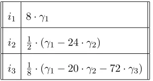
2.3. Efficacy of the absolute Igusa invariants. The so-called absolute Igusa invariants are the functions
i1 =A5/D, i2=A3B/D, i3 =A2C/D.
The choice of terminology is somewhat unfortunate, as it leads one to think that these invariants determine the isomorphism class of the curve; we’ll discuss it further below.
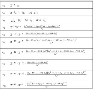
SinceD= 212J10, the functionsi1, i2, i3,belong toR⊗Z[1/2]. It is a consequence of the results
mentioned so far that the functions γj are rational functions of the functions ij and vice-versa.
This calculation is presented in the following two tables.
Table 2.3.1. The absolute Igusa invariantsi1, i2, i3 in terms of the generators γj
i1 8·γ1
i2 12 ·(γ1−24·γ2)
i3 18 ·(γ1−20·γ2−72·γ3)
An interesting consequence of this calculation is that the natural map
M2⊗Z[1/6] = Spec(R⊗[1/6])−→Spec(Z[1/6][i1, i2, i3]) =A3Z[1/6],
can be inverted whenever i1 6= 0. However, given a triple (i1, i2, i3), which is in the image of the
map, and such that i1 = 0, we find thatA= 0 and hence also that i2 =i3= 0. Thus, there is a
unique point ofA3, which is in the image, for which we cannot invert the map and it corresponds
to all the genus 2 curves for which A= 0. Thus, the absolute Igusa invariants fail to completely determine the isomorphism class of the curve, but only if i1= 0.
The vanishing locus ofA is a surface inM2. There is a natural immersion,
ρ:M2 −→A2,1,
of the moduli space of curves M2 to the moduli space of principally polarized abelian surfaces
with no level structureA2,1, sending a curve to its canonically polarized Jacobian. The image is
the complement of the Humbert surface H1, which is the divisor of the modular form Θ defined
below. Via this map, each of the Igusa invariants is, in a suitable sense, a pull-back via ρ of a meromorphic Siegel modular form whose polls are supported on H1. These modular forms were
calculated by Igusa [Igu3, p. 177-8] and the reader is referred to this reference for details. The invariantDis the pullback of a scalar multiple of Θ, defined in page 12. There is a modular form of weight 12, which Igusa denotesχ12, such that, in a suitable sense,Ais a scalar multiple of the
weight 2 meromorphic form χ12/Θ. We have thus, as sets,
{A= 0}=ρ−1{χ12= 0}.
The modular form χ12 is a cusp form (see [Igu2, p. 195]). However, there does not seem to be
Table 2.3.2. The generatorsγj in terms of the absolute Igusa invariantsi1, i2, i3
(the last column gives the denominator)
γ1 2−3·i1
γ2 2−63−1·(i1−16·i2)
γ3 34561 ·(i1+ 80·i2−384·i3)
γ4 2−113−3· i1
2+416·i
1i2−1536·i1i3−768·i22
i1
γ5 2−10·3−4· (i1−16·i2)(i1+80·i2−384·i3)
i1
γ6 2−25·3−7· (i1−16·i2)(i12+416·i1i2−1536·i1i3−768·i22) 2
i13
γ7 2−22·3−9·
(i1+80·i2−384·i3)2(i12+416·i1i2−1536·i1i3−768·i22)
i12
γ8 2−29·3−15· (i1+80·i2−384·i3)5
i12
γ9 2−37·3−12·
(i1+80·i2−384·i3)(i12+416·i1i2−1536·i1i3−768·i22)3
i14
γ10 2−52·3−15· (i12+416·i1i2−1536·i1i3−768·i22) 5
i16
Proposition 2.3.1. Let V ⊆ A2,1(C) be the support of the divisor of χ12. There are finitely many primitive CM points on V, that is, CM points associated to primitive CM fields of degree four.
Proof. Let S be the collection of all primitive CM points on V. We note that the description of M2 implies thatV is irreducible. LetC be the Zariski closure of S. If S is infinite then C is
either a curve, or V itself. In either case, it follows from the Andr´e-Oort conjecture, known to be true under GRH by the work of Klinger-Yafaev [Yaf], that C is either a Shimura curve, or a Shimura surface. It remains to review the possibilities: (i) ifCis a Shimura curve then every CM point on C is coming from a bi-quadratic (equivalently, non-primitive) CM field of degree 4; (ii) if C =V then V is a priori in the Hecke orbit of some Humbert surfaces, but that Hecke orbit is a union of Humbert surfaces (this follows easily from the moduli interpretation). Since the Humbert surfaces inA2,1 are irreducible,V is a Humbert surface itself, which is not the case.
2.4. Igusa class polynomials. In [GL1,§5.2] it was explained how the absolute Igusa invariants can also be expressed in terms of Siegel modular functions. We summarize this here for the reader’s convenience.
The Igusa functionsi1,i2,i3can be defined as rational functions in Siegel Eisenstein series,ψw,
of weights w = 4, 6, 10, 12. To begin with, the cusp forms Θ and χ12, of weights 10 and 12,
and [Igu4, p. 848]):
−2−2Θ =χ10=
−43867
212·35·52·7·53(ψ4ψ6−ψ10)
and
χ12=
131·593
213·37·53·72·337(3
2·72ψ3
4+ 2·53ψ62−691ψ12).
Then the Igusa functions i1, i2, i3 can be expressed as
i1= 2·35
χ512
χ610, i2 = 2
−3·33ψ4χ312
χ410 , i3 = 2
−5·3ψ6χ212χ10+ 22·3ψ4χ312
χ410 .
(These are often called j1,j2,j3 in the literature, but we stick with Igusa’s notation.)
Let K be a primitive, i.e. not biquadratic, CM field of degree 4 over Q. We define the Igusa class polynomialsto be:
(2.4.1) h1(x) =
Y
τ
(x−i1(τ)), h2(x) =
Y
τ
(x−i2(τ)), h3(x) =
Y
τ
(x−i3(τ)),
where the product is taken over allτ ∈Sp(4,Z)\H2, such that the associated principally polarized
abelian variety has CM by OK. One can define other absolute invariants, called j1, j2, j3, as
in [GL1, p. 473], where it is also remarked that i1 = 2−12j1 and i2 = 2−12j2, and then we define
the corresponding class polynomials as follows:
(2.4.2) hi(x) =Y
τ
(x−ji(τ)), i= 1,2,3.
The advantage of using these is that it is clear from their definition that they satisfy the hypotheses of our Main Theorem.
2.5. Rosenhain normal form. While Igusa’s approach to the moduli of genus 2 curves is through the study of invariants of sextics, we remark that after a finite extension of the base we may always arrange the six ramification points to contain {0,1,∞}and arrive at an equation of the form
(2.5.1) C:y2 =x(x−1)(x−λ1)(x−λ2)(x−λ3),
called the Rosenhain normal form of the curve C. The λi’s are in a finite field extension of the
field of definition of the curve and are determined up to the action of the stabilizer of the triple {0,1,∞} in PGL2 a group isomorphic to the symmetric groupS3 on 3 letters. If τ ∈H2 is the
period matrix of the polarized abelian surface Jac(C), then, up to projective equivalence we may take the λi to be
λ1=
Θ 1 1 0 0
(τ)2 Θ
1
0 0 0
(τ)2
Θ 0 1 0 0
(τ)2 Θ
0
0 0 0
(τ)2
, λ2 =
Θ 1 0 0 1
(τ)2Θ
1
1 0 0
(τ)2
Θ 0 0 0 1
(τ)2Θ
0
1 0 0
(τ)2
, λ3 =
Θ 1 0 0 1
(τ)2 Θ
1
0 0 0
(τ)2
Θ 0 0 0 1
(τ)2 Θ
0
0 0 0
(τ)2
.
(See [Igu2, p. 179].) Note that if C is defined over some number field and the equation (2.5.1) is over that field then the λi appearing there are algebraic numbers. When obtaining a triple of
λi from the period matrix the λi are in fact algebraic. This is a consequence of the fact that the
ratios of the theta functions appearing above are modular functions defined over Q(i) (say) and
The theta functions used here are Riemann’s theta functions: Let, 0 ∈Qg,τ ∈Hg, and define
the Riemann theta function withcharacteristic [0] to be the power series
Θ [0] (τ) =
X
N∈Zg
e
1 2
tN +
2
τN + 2
+tN + 2
0
2
,
where e(x) = e2πix. It can be shown that this series defines a holomorphic function Hg → C.
If , 0 ∈ Zg they are called an integral characteristic. If t0 ≡0 (mod 2) they are called even, and else odd. It turns out that for an odd characteristic the theta function vanishes identically, and for even characteristic Θ [0] (τ)2 depends only on (, 0) modulo Z2g. For g = 1 this gives us 3 (squares of) theta functions and forg= 2 this gives us ten (squares of) even theta functions. One can show that each Θ [0] (τ) to a large enough even power 2r is a Siegel modular form of weight r of some level. For g= 1, it goes probably to Jacobi that
∆ =c Y
[0]even
Θ [0] (τ)4,
where c is a constant and ∆ =E43−E62 is the classical modular form of weight 12. Recall that the divisor of ∆ is the cusp of SL2(Z)\H. Igusa proved for g= 2 that
Θ := 2−12 Y [0]even
Θ [0] (τ)2
is a Siegel modular form of level Sp(4,Z) and weight 10. The factor of 2 is introduced to ensure
integral Fourier coefficients with gcd 1. The divisor of Θ is precisely the Humbert divisor H1
(with multiplicity 2). See §4.
Finally, we make some remarks as the utility of the Rosenhain normal form for generating curves of genus 2 with CM. Given a primitive CM fieldK, it is an easy matter to enumerate representatives for the ideal classes of K and so to get, by varying over all CM types, the period matrices whose classes modulo Γ(2) give all the CM points of level 2 associated to this field. The modular forms used above are of level 2 and so, by evaluating them on these period matrices, we get a collection of equations C :y2 =x(x−1)(x−λ1)(x−λ2)(x−λ3) defining, in particular, the isomorphism
classes of all the curves of genus 2 whose Jacobians have CM byOK. For ageneric period matrix
τ ∈H2 the λi(τ) live in a very large extensionL of the field of definition, say L0, of the curve.
LetL0 =L(√λ1,
√ λ2,
√
λ3); note that [L0 :L]≤8. Implicit in the fact thatλi∈Lis that all the
2-torsion of Jac(C) are defined over L0, because under the embedding C →Jac(C) (taking the point at infinity as the base point) the images of the Weierstrass points generate the 2 torsion subgroup of Jac(C). For a generic curve, the extension L0/L0 has degree] Sp(4,Z)/Γ(2) = 720.
However, in the case of complex multiplication, the field of definition ofCcan be takenHK∗, the Hilbert class field of the reflex field, and so the λi generates the ray class field of conductor 2 of
K∗. In fact, since Sp(4,Z)/Γ(2) ∼= Sp(4,F2) ∼= S6, the symmetric group on 6 letters, and since
the maximal abelian subgroups of S6 have degrees 5,6,8,9, it follows that [L0 : L0]|a for some
a ∈ {5,6,8,9}. This can be utilized to construct curves over a number fields whose Jacobians have CM.
2.6. Ramification locus of A2,N(C)→A2,1(C). Let N be a positive integer. We denote
by A2,N the moduli scheme of principally polarized abelian surfaces with symplectic level N
Sp(4,Z/NZ)/{±I4}. We denote the byH∆,N the Humbert surface of invariant ∆ (a discriminant
of real quadratic order) inA2,N(C). It is irreducible forN = 1, but reducible forN >1.
Let N ≥3, so the representation Aut(A, λ)→Aut(A[3]) is faithful. The ramification locus of πN :A2,N →A2,1 is clearly the locus of points x on A2,1 with non-trivial stabilizers, which, by
the moduli interpretation, correspond to principally polarized abelian surfaces (A, λ) such that rAut(A, λ) 6={1}, where rAut is the reduced automorphism group (namely the automorphisms ϕ:A→A such thatϕ∗λ=λ, taken modulo{±1}). Furthermore, in that case, any point in the fibre over x has the same ramification index, equal to the cardinality of rAut(A, λ).
We say that a component of the Humbert divisorH∆,N inA2,N(C) is ramified if it is contained
in the ramification locus and otherwise we say it is unramified. If every component of H∆,N is
unramified then
π∗N(H∆,1) =H∆,N.
Lemma 2.6.1. If∆6= 1,4every component ofH∆,N is unramified. If∆∈ {1,4}the ramification index along each component of H∆,N is2.
Proof. Suppose first that ∆ is not a square. In this case, every abelian variety (A, λ) parameter-ized byH∆,N has real multiplication by a real quadratic order of discriminant ∆ and, generically,
only by that order. Thus, generically, Aut(A, λ) ={±1}(as the Rosati involution is the identity). That resolves this case.
Suppose now that ∆ is a square, but ∆ 6= 1. Then. except of codimension one subset, the points of H∆,N correspond to curves C of genus 2 affording a map of degree ∆, C →E, to an
elliptic curve E, that does not factor non-trivially thorough another elliptic curve [FK].
From Igusa’s classification of Aut(C) we deduce that there is only one 2-dimensional family of curves of genus 2 with a non-trivial reduced automorphism group. This family, as one observes, is exactly the curvesC of genus 2 allowing a map of degree 2,C→E, to an elliptic curve, ramified at exactly two points of E. This family is the Humbert divisor H4,1, and in particular, we have
proven the lemma for all cases but ∆ = 1.
It is easy to see that for a generic pair of elliptic curvesE1, E2 we have Aut(E1×E2, λ1×λ2) =
{(±1,±1)}. Thus, our proof is complete.
2.7. Existence of good models for abelian varieties with complex multiplication. Our purpose is to prove the following lemma.
Lemma 2.7.1. Let (A, λ) be a g-dimensional principally polarized complex abelian variety with complex multiplication by the ring of integersOK of a CM fieldK of degree2g,ι:OK →End(A). Let Φ be the associated CM type and K∗ the reflex field associated to K and Φ. Assume that Φ
is a simple CM type. Let p be a prime of K∗ and R the completion of the ring of integers of K∗
by p. Then (A, λ, ι) has a model with good reduction over an unramified extension O of R. Proof. As is well known ([Lang1, Ch. 3, Thm. 1.1]), (A, ι, λ) has a model overHK∗, the Hilbert class field of K∗, corresponding to anHK∗-rational point a∈Ag,1. In fact,ais defined over the field of moduli M of (A, ι, λ) which is contained in HK∗. Let N ≥3 be an integer prime to p. Let ˜a be a point of Ag,N lying above a. The field of definition of the point ˜a is contained in
HK∗(A[N]) and is equal to the field of moduli M[N] of (A, ι, λ, A[N]), which, since the moduli scheme is a fine moduli scheme, is also the field of definition of (A, ι, λ, A[N]).
Let Ag,N† be a smooth toroidal compactification of Ag,N over Spec(Z[ζN,1/N]). It carries
a semi-abelian variety X over it. Choose a prime P of M[N] over p. Since the morphism A†
the valuative criterion a morphismβ : Spec(O)→Ag,N† , whereOis the valuation ring ofM[N]P. Then β∗X is a principally polarized semi-abelian variety over O whose generic fiber is (A, λ)⊗ M[N]P (ιextends automatically). As is well known, since [K :Q] = 2g > g, the toric part of the
mod Preduction of β∗X must be trivial and soA⊗M[N] has good reduction moduloP. We claim that the extensionM[N]/K∗ is unramified atpand so Ois an unramified extension ofR. This follows from the main theorems of complex multiplication. In factM[N] is an abelian extension ofK∗ corresponding to a precisely described group of ideals and has conductor dividing N. See [Lang1], Chapter 5, Theorem 4.3 (use also Theorem 3.3). Thus, the extension M[N]/K∗
is unramified at p.
Remark 2.7.2. In fact, using more subtle results in complex multiplication due to Shimura, one can conclude the existence of a model over HK∗ with good reduction atp. See [Gor, Proposition 2.1].
Remark 2.7.3. The abelian variety (A, ι, λ) has a model overHK∗, but this model is not unique. In fact, the forms of (A, ι, λ) over HK∗ are classified, up to HK∗ isomorphism, by the Galois cohomology group H1(G
HK∗,Aut(A, ι, λ)), where GHK∗ is the absolute Galois group of HK∗
and Aut(A, ι, λ) are the automorphisms commuting with the action of K and preserving the polarization. It is easy to see that Aut(A, ι, λ) is equal to µK, the group of roots of unity lying
inK. Typically this group is {±1} and the forms correspond to quadratic twists, but it may be larger. It can be µt for any t such that ϕ(t)|2g. On the other hand, with accordance with the
fine moduli space property (A, ι, λ, A[N]) has no forms as Aut((A, ι, λ, A[N])) ={1} forN ≥3.
3. Reduction type of abelian surfaces with complex multiplication
Our goal in this section is to study the reduction type of an abelian surface with complex multi-plication by a fieldK modulo a prime ideal of the field of definition, lying above p, as a function of the decomposition of the prime p inK
3.1. Combinatorics of embeddings and primes. LetK be a number field and N its normal closure over Q. Let Gbe the Galois group Gal(N/Q), acting on K by k7→g(k), g∈G, and let
H = Gal(N/K)< G. Fix inclusions
ϕC:N →C, ϕp:N →Qp.
This allows us to make the following identifications:
Hom(K,C) =ϕC◦G/H, Hom(K,Qp) =ϕp◦G/H,
where a left coset gH gives the embeddingsϕC◦g andϕp◦g. We then have an identification
Let L⊇N be a finite extension and choose an extension of ϕC, ϕp to L. We have the following
diagram:
L ϕC(ϕp)//C(Qp)
N
ssssss
sssss
K K K K K K K K K K
K
J J J J J J J J J J
J K∗
tttttt
ttttt
Q
LetPbe the maximal ideal ofQp. The choice ofϕpprovides us with a prime idealpL,1 :=ϕ−p1(P)
of L, and so with prime ideals pN,1 =pL,1∩N of N and pK,1 =pL,1∩K of K. Let D be the decomposition group of pN,1 inN and I its inertia group. Lete=] I. The primes ideals above
p inN are in bijection with the cosetsG/D: pON =
Y
α∈G/D
peN,α, pN,α =α(pN,1).
The decomposition (respectively, inertia) group of pN,α is Dα := αDα−1 (respectively, Iα := αIα−1). The primes dividing pinK correspond to the double cosets H\G/D. More precisely,
pOK= Y
HαD∈H\G/D
pe(α)K,α, pK,α=α(pN,1)∩K,
where, by Lemma 3.2.1 below,e(α) = [Iα :Iα∩H].
Letα∈G; it induces a homomorphismϕp◦α:K →Qp that depends only onαH. It therefore
defines a prime (ϕp◦α)−1(P) ofK, or more precisely (ϕp|K◦α)−1(P). We have
(3.1.1) (ϕp|K◦α)−1(P) = (α−1ϕp|−N1(P))∩K =α−1(pN,1)∩K=pK,α−1.
That is, the coset αH corresponding to an embedding K →Qp induces the prime corresponding to the double coset Hα−1D. (This “inversion” is a result of our definition of pN,α asα(pN,1), as opposed to α−1(pN,1), made in order to conform with [Gor].)
Suppose that we are given a finitely generated torsion free OL-module M on which OK acts as endomorphisms. Then MC = M⊗OL,ϕC C is a finite dimensional vector space over C, which is
an OK⊗ZC=K⊗QCmodule. We have then a decomposition
(3.1.2) MC=⊕ϕ∈Hom(K,C)MC(ϕ) = Homα∈G/HMC(α),
where MC(ϕ) is the eigenspace for the character ϕ: K→C, where, using the identifications Hom(K,C) = Hom(K, N) = G/H, we have let MC(α) := MC(ϕC◦α). We assume that each
eigenspace is either zero or one dimensional and so we get a subset Φ⊂Hom(K, N),
On the other hand, we also have the finite dimensional Qp-vector space Mp :=M⊗OL,ϕpQp,
grace of the homomorphism ϕp:L→Qp, which is an OK ⊗ZQp =K⊗QQp-module. Since all
the homomorphismsK →Qp factor as K →N ϕp
−→Qp,we have a decomposition, similar to the
one in (3.1.2),
(3.1.3) Mp=⊕ϕ∈Hom(K,Qp)Mp(ϕ) =⊕α∈G/HMp(α).
Moreover, for each α ∈G/H there is a one dimensional L-subspace ML(α) of ML :=M ⊗OLL
such that
MC(α) =ML(α)⊗L,ϕCC, Mp(α) =ML(α)⊗L,ϕpQp.
And so, in the obvious sense, Φ becomes a “p-adic CM type” as well.
Now, the decomposition in (3.1.3) can be packaged as follows: We haveOK⊗ZZp =⊕p|pOKp and thus K⊗QQp =⊕p|p(Kp⊗QpQp), or
K⊗QQp=⊕α∈H\G/D(KpK,α⊗QpQp).
This decomposition induces a decomposition
(3.1.4) Mp =⊕α∈H\G/DMp,α.
Note that, due to (3.1.1), the relation between (3.1.3) and (3.1.4) is (sic!)
(3.1.5) Mp(α)⊆Mp,α−1.
3.2. The case of quartic fields and Dieudonn´e modules. Let K be a CM field of degree four over the rational numbers and letA be a principally polarized abelian surface with complex multiplication byOK, CM type Φ, defined over a fieldL and having everywhere good reduction. Let K∗ be the reflex field. We assume that L contains a normal closure N of K and let G = Gal(N/Q). Thus, our notation conforms with the one in the previous section.
LetK+be the totally real subfield ofK. Letpbe a prime number. Our purpose is to determine
the reduction ¯A ofA modulo a prime idealpLof L. It follows from results of C.-F. Yu [Yu] that the Dieudonn´e module of ¯A is determined uniquely by Φ and the prime decomposition of p in K (and not just in the case of surfaces). A fortiori, the Ekedahl-Oort strata in which it falls is determined. In the case of surfaces, the complete information is contained in two numbers
a( ¯A) = dim Hom
Fp(αp,
¯
A⊗Fp), f( ¯A) = logp]A[p](Fp),
the a-number and f-number.
We the situation more explicit that in loc. cit., and provide a self-contained proof in our case. We will have several fields to consider N,K, K∗ (the reflex field determined byK and Φ), and their totally real subfields K+ and K∗+, respecively. The basic information is the factorization of p inN. As above, we fix a prime ideal p= pN,1 =pL∩N of N. The decomposition of p in each field is determined by the pair of subgroups (I, D), where I is the inertia group of p in N and D is its decomposition group. The pair of subgroups (I, D) of Gal(N/Q) must satisfy the
two restrictions: • ICD;
As explained above, having chosenp, we may index the primes dividingpinN by coset represen-tatives forDinG. If these coset representatives area, b, c, . . . (soG=aDtbDtcDt. . .) then we write pON =peN,apeN,bpeN,c· · ·, where e=]I and pN,a:=a(pN) (and in particular, pN,1 =p).
If the primes appearing in the decomposition of pinN are determined by G/Dthen the primes appearing in the decomposition ofpin a subfieldNH ofN, corresponding to a subgroupHofG, are determined by H\G/D. As above, we shall denote such primes bypNH,x wherex is a
repre-sentative for a double coset HxD. (This is consistent with the previous notation for H ={1}.) The following lemma is used to determine ramification in subfields.
Lemma 3.2.1. Let Q⊂B ⊂N be three number fields where N/Q is Galois with Galois group
G. Let B correspond to a subgroup H of G. Let pN be a prime ideal of N, pB =pN ∩B and pQ=pN ∩Q. LetI(pN) be the inertia group inG. Then,
e(pB/pQ) = [I(pN) :I(pN)∩H]
and
e(pN/pB) =] I(pN)∩H.
Proof. This is Lemma 3.3.29 in [Coh].
The main tool for studying the reduction ¯A = A (mod pL) of the abelian surface A is the following. LetDbe the Dieudonn´e module of ¯A[p] overFp. The formalism of the previous section
will be applied to the algebraic first de Rham cohomology of A/L, serving asM in the previous section, which by base change gives us the complex de Rham cohomology of A as well as the crystalline cohomology of ¯A, of whichDis the reduction modulop.
Thea-number andf-number of ¯Acan of course be read fromD. The Dieudonn´e module has a
decomposition relative to theOK+ action and a refined decomposition relative to theOK action.
Using pK+ to denote a prime ideal of OK+ above p and similarly for pK, we have, by virtue of
the decompositions OK+⊗Zp =⊕p
K+OK+,pK+,OK⊗Zp=⊕pKOK,pK, induced decompositions
D=⊕pK+D(pK+), D(pK+) =⊕pK|pK+D(pK).
Here each D(pK+) is a self-dual Dieudonn´e module of dimension 2e(pK+/p)f(pK+/p), which is
then decomposed in Dieudonn´e modulesD(pK) of dimensione(pK/p)f(pK/p). OnD(pK+) there
is an action of OK+,p
K+ ⊗Fp
∼
=⊕αFp[t]/(te), where the summation is over embeddingsα of the maximal unramified subringOur
K+,p
K+ of
OK+,p
K+ intoW(Fp) ande=e(pK+/p). There is a
simi-lar and compatible decomposition ofOK,pK⊗Fp. These decompositions induce decompositions of
the Dieudonn´e modulesD(pK+),D(pK), such thatD(pK+) =⊕αD(pK+, α),D(pK) =⊕αD(pK, α). D(pK+, α) is a vector space of dimension 2e(pK+/p), which is a free rank 2 module overFp[t]/(te)
on which OK+,p
K+ =O
ur K+,p
K+[π] acts via the map ¯α :O ur K+,p
K+ →Fp and π, which is an
Eisen-stein element, acts viat. A similar and compatible description is obtained forD(pK, α). Frobenius
induces mapsD(pK+, α)→D(pK+, σ◦α).
Implicit in our considerations is the identification of Hom(K, N) with Hom(K,Qp), whereN is a
normal closure ofK. This identification is done as discussed in detail above. In particular, we note that the subspace D(pK, α) is associated with the prime ideal pK,α−1. Since H0( ¯A,Ω1¯
A,Fp)
⊂D, any α ∈Φ contributes 1 to the dimension of the kernel of Frobenius on D(pK,α−1). This often
allows us to conclude that Fr2 = 0 on D, which implies a = 2, f = 0 and, so, superspecial
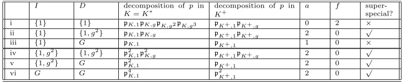
Table 3.3.1. Reduction in the cyclic case.
I D decomposition of p in
K=K∗
decomposition of p in
K+
a f
super-special? i {1} {1} pK,1pK,gpK,g2pK,g3 pK+,1pK+,g 0 2 ×
ii {1} {1, g2} p
K,1pK,g pK+,1pK+,g 2 0
√
iii {1} G pK,1 pK+,1 1 0 ×
iv {1, g2} {1, g2} pK,12 p2K,g pK+,1pK+,g 2 0
√
v {1, g2} G p2K,1 pK+,1 2 0
√
vi G G p4K,1 p2
K+,1 2 0
√
Another useful tool to quickly decide some properties of the reduction is the following relation. LetK∗ be the reflex field defined by the CM type of the abelian variety under consideration and let Φ∗ be the reflex type. LetpK∗,1=pN,1∩K∗. Then some power of NormΦ∗(pK∗,1) is equal to a power of Fr, viewed as endomorphisms of the reduction. One can be more precise (see [Lang1]), but we note that this suffices to calculate the f-number of the reduction.
3.3. K cyclic Galois. In this caseK =N =K∗. The Galois group is cyclic of order 4, generated by g, say, where g2 is complex conjugation. The CM types are either {1, g},{g, g2},{g2, g3} or
{g3,1}. Since the reduction type does not depend on the way K is embedded in A, namely we
can compose with an automorphism K →K, we may assume that the CM type is{1, g}. The reflex CM field K∗ isK and Φ∗ ={1, g−1}. We have the following possibilities.
The unramified case appears in [Gor], but we shall do one case to illustrate our method. Consider the case ii. We have a decomposition
D=D(pK+,1)⊕D(pK+,g),
and D(pK+,i), i = 1, g, is a two dimensional Fp-vector space that does not decompose further
relative to the OK+ action. However, D(pK+,i) =D(pK,i), because pK+,i is inert in K, and
D(pK,i) =D(pK,i, α)⊕D(pK,i, σ◦α).
Frobenius takes D(pK,i, α) toD(pK,i, σ◦α), and vice-versa. The CM type is {1, g}and we note
thatgswitchespK,1 andpK,g. This means that the cotangent space, or ratherH0(A,Ω1
A/Fp
)⊗
Fp,σ
Fp =D(Ker Fr), which is an OK-module, is not contained completely in any of D(pK,i). Thus,
Frobenius has a kernel on each of D(pK,i). It follows that Fr2 is zero on eachD(pK,i) and hence
on Dand that implies that a( ¯A) = 2, by a well known and elementary argument andf( ¯A) = 0.
In case iv we again have
D=D(pK+,1)⊕D(pK+,g),
and D(pK+,i) is a two dimensional Fp-vector space that does not decompose further relative
to the OK+ action. However, D(pK+,i) = D(pK,i) and D(pK,i) becomes a rank 1 module over Fp[t]/(t2) by using theOK action and Frobenius is a module homomorphism. Once more, since
g permutespK+,1 andpK+,g, it follows that Frobenius has a kernel on each ofD(pK+,i) and since
the dimension of the kernel of Frobenius is two, it follows that the kernel Frobenius must be (t)⊕(t)⊂D(pK,1)⊕D(pK,g) and Fr2 = 0.
In case v, after a similar analysis we reach the conclusion that D = Fp[t]/(t2)⊕Fp[t]/(t2)
and that Frobenius, which commutes with the Fp[t]/(t2) structure, permutes the components.
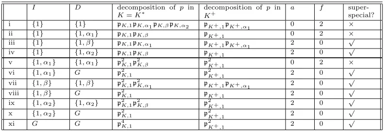
Table 3.4.1. Reduction in the bi-quadratic case.
I D decomposition of p in
K=K∗
decomposition of p in
K+
a f
super-special? i {1} {1} pK,1pK,α1pK,βpK,α2 pK+,1pK+,α1 0 2 ×
ii {1} {1, α1} pK,1pK,β pK+,1 0 2 ×
iii {1} {1, β} pK,1pK,α1 pK+,1pK+,α1 2 0
√
iv {1} {1, α2} pK,1pK,β pK+,1 2 0
√
v {1, α1} {1, α1} p2K,1p 2
K,β p
2
K+,1 0 2 ×
vi {1, α1} G p2K,1 p
2
K+,1 2 0
√
vii {1, β} {1, β} p2K,1p2K,α
1 pK+,1pK+,α1 2 0
√
viii {1, β} G p2
K,1 pK+,1 2 0
√
ix {1, α2} {1, α2} p2K,1p2K,β p2K+,1 2 0
√
x {1, α2} G p2K,1 p2K+,1 2 0
√
xi G G p4K,1 p2K+,1 2 0
√
Fr2 = 0 (in fact, taking into consideration the CM type we must have the kernel is (t)⊕(t), but this is not important at present).
In case vi we conclude that D = Fp[t]/(t4) and that Frobenius acts as a Fp[t]/(t4)-module
homomorphism. It follows that the kernel of Frobenius, being anFp[t]/(t4)-module is (t2) and so
is the image. Hence Fr2 = 0 again.
3.4. K biquadratic. In this case K = N is the compositum K1K2 where Ki are quadratic
imaginary fields. LetK+be the totally real subfield ofK. Write the Galois group is{1, α1, α2, β}
where Ki is fixed by αi and β is complex conjugation. We have the following diagram:
K hα1i
zzzzzz
zz
hβi hα2i D D D D D D D D
K1
C C C C C C C
C K+ K2
{{{{{{
{{
Q
The possible CM types are{1, αi},{β, αi}and twisting the action ofOK by an automorphism we may assume the CM type is{1, α1}or{1, α2}. The situation being symmetric we assume w.l.o.g
that the CM type is {1, α1}. The reflex CM field is K1 and the reflex CM type is {1}. In this
case A is isogenous to E⊗ZOL, or equivalently to E⊗K1 K, whereE is an elliptic curve with
CM byOK1. Thus, ¯Ais ordinary ifpis split inK1 and supersingular otherwise (and in that case
one still needs to figure out itsanumber). Now, pis split inK1 if and only ifhD, α1i 6=G.
Consider for example case vi. After the usual analysis we find that D ∼=Fp[t]/(t2)⊕Fp[t]/(t2),
where Fr is Fp[t]/(t2) σ-linear and switches the components. Its kernel is then either one of the
components, or the submodule (t)⊕(t). In any case, Fr2 = 0 and so a= 2. Cases vii, viii and x lead exactly to the same setting.
In case ix, once againD∼=Fp[t]/(t2)⊕Fp[t]/(t2) but now Fr acts on each component separately.
¯
Ais ordinary if the kernel of Fr is one of the components and is superspecial if the kernel is (t)⊕(t). Since ordinary is not possible, because p is inert inK1 (or, we can argue by using the CM type
In case xi we find that D ∼= Fp[t]/(t4) and we must have that the kernel of Frobenius is the
submodule (t2). It follows that Fr2 = 0.
3.5. K non-Galois. In this case the normal closure of K is a Galois extensionN/Qof degree 8
and Galois groupD4. As above, we viewN as embedded inC. Kis the fixed field of a non-central
involution we call x. Let y be an element of order 4, theny2 is complex conjugation and xyx= y−1=y3. We identify Hom(K,C) with{1, y, y2, y3}and the CM types are{1, y},{y2, y3},{1, y3}
and {y2, y3}. We may twist the action ofK by complex conjugation and so assume that the CM
type is {1, y} or {1, y3}. If it is {1, y−1} we can change the presentation of our group by using
the generator y−1 instead ofy. We can therefore assume that K is fixed by x, the Galois group is hx, y|x2, y4, xyxyi and the CM type is{1, y}. The reflex CM fieldK∗ is then fixed by{1, xy3}
(follow the recipe in [Lang1, Ch. 1, Theorem 5.1]) and the reflex CM type is{1, y−1}.
We have the following diagrams of fields and subgroups:
{1}
{1, x}
m m m m m m m m m m m m m m m
{1, xy2}
{ { { { { { { {
{1, y2} {1, xy}
BBBB BBBB
{1, xy3}
QQQQQQQQQQQQ
{1, x, xy2, y2}
m m m m m m m m m m m m m z z z z z z z z
{1, y, y2, y3} {1, xy, y2, xy3}
QQQQQQQQQQQQ Q DDDD DDDD G m m m m m m m m m m m m m m RRRRRRR RRRRRRRR N K m m m m m m m m m m m m m m m
m · · ·
N+ · · · K∗
RRRRRRR RRRRRRRRR K+ m m m m m m m m m m m m m m m
· · · K∗+
QQQQQQQ QQQQQQQQ Q m m m m m m m m m m m m m m m QQQQQQ QQQQQQQQQ
The analysis of the reduction ofAproceeds along the same lines as above. Namely, one considers the decomposition of the Dieudonn´e module as a module overOK⊗Fp and the induced action
of Frobenius, which is 1⊗σ-linear, so to say. In most cases, this suffices to determine theaand f numbers, but in certain cases one needs to decide between two possibilities, and there the CM type matters. The interpretation of the CM type mod p is done through the formalism of§3.1.
For example, referring to the table, in case viii we find that D ∼= Fp[t]/(t2)⊕Fp[t]/(t2) and
Frobenius acts σ-Fp[t]/(t2) linearly (meaning, it acts σ-linearly on Fp and commutes with t) on
each component. The kernel, a-priori could be one of the components or the submodule (t)⊕(t). Taking the CM type into consideration, we see that Frobenius has a kernel in each component and so its kernel is (t)⊕(t). It follows that Fr2 = 0. Case x is the same.
Case ix is easier as in this caseD∼=Fp[t]/(t2)⊕Fp[t]/(t2), where Fr is actingσ-Fp-linearly, but
3.6. Examples. Take a curve C of genus 2 over Q (to simplify). Given a prime p at which C
has good reduction ¯C, one has a simple method of writing down the Hasse Witt matrix M of ¯
A = J ac( ¯C) and so deciding the a number and f number of ¯A: The f number is the rank of M(p)M and thea-number is the co-rank ofM. In general it is hard to decide the reduction type by examining M, but in certain cases we can do that and compare our results with the results above whenA= Jac(C) has complex multiplication.
Let C:y2=f(x), where f(x) =x5+a4x4+· · ·+a0 be a hyperelliptic curve and write
f(x)(p−1)/2=X
j≥0
cjxj.
Then the Hasse-Witt matrix M is given by
cp−1 cp−2
c2p−1 c2p−2
,
and M(p) is
cpp−1 cpp−2 cp2p−1 cp2p−2
.
Exactly the same recipe works if f(x) is a sextic. See [IKO, p. 129]
3.6.1. LetC :y2 =x5+ 1. The curve has good reduction outside 2·5. The Jacobian has complex
multiplication by Q(ζ5) and the automorphism group of the curve in characteristic zero is µ10.
The coefficient of xn in f(x)(p−1)/2 is 0 if 5 -n and, for n not larger than 5(p−1)/2 such that
5|n, is (p−n/51)/2
. We divide the analysis to several cases:
• If p ≡ 1 (mod 5), M =
((p−1)/2
(p−1)/5) 0
0 ((p−1)/2
(2p−2)/5)
has rank 2 and we conclude that ¯A is ordinary. Note thatpsplits completely in this case. Namely we are in case i of the cyclic Galois case.
• Ifp≡2 (mod 5), p >2,M =0((p(p−−1)/22)/5)
0 0
has rank 1 and M(p)M = 0. Thus,f = 0 and
a= 1. This is a supersingular, but not superspecial reduction, in accordance to case iii. • Ifp≡3 (mod 5),M =
0 0
((p−1)/2
(2p−1)/5)0
has rank 1 andM(p)M = 0. Thus,f = 0 anda= 1. This is a supersingular, but not superspecial reduction, in accordance to case iii again. • Ifp ≡ −1 (mod 5), M = (0 00 0) has rank 0 and we have superspecial reduction, in
accor-dance with case ii.
• p= 5. It follows from Igusa’s classification of genus 2 curves with many automorphisms [Igu1, §8] that the reduction of a stable model of y2 = x5+ 1 modulo 5 is isomorphic, possibly after base change, to the curvey2=f(x), wheref(x) =x(x−1)(x+1)(x−2)(x+ 2). That is, since the characteristic is 5,f(x) =x5−x. Thenf(x)2 =x10−2x6+x2 and the Hasse-Witt matrix is the zero matrix, giving us superspecial reduction. This agrees with case v.
3.6.2. Consider the curvey2=−8x6−64x5+ 1120x4+ 4760x3−48400x2+ 22627x−91839, which
has complex multiplication by the ring of integers ofK =Q(
p
−65 + 26√5) by [Wam]. The field is a cyclic Galois extension with a totally real fieldK+ =Q(
√
5). Its discriminant is 53·132. The prime 5 decomposes asp2K+ =pK4 and belongs to case vi, the prime 13 decomposes asqK+ =q2K
and belongs to case v. In any case, we have superspecial reduction. And, indeed, in both cases one finds that the Hasse-Witt matrix is identically zero modulo the corresponding prime. For example, forp= 5 we have f(x)2= 64x12+ 1024x11−13824x10−219520x9+ 1419520x8+ 16495568x7− 87185232x6 −398328128x5 + 2352249680x4 −3064600880x3 + 9401996329x2−4156082106x+ 8434401921 and the Hasse-Witt matrix is 2352249680−219520 −30646008801419520 ≡0 (mod 5).
3.6.3. Cases (v) and (vi) in Table 3.3.1 for Galois cyclic fields. Examples 1 and 2 below demon-strate cases (v) and (vi) in the table for Galois cyclic fields. For both, we take the Galois cyclic fieldK =Q[x]/(x4+ 238x2+ 833), with real quadratic subfieldQ(
√
17). It can be constructed by adjoiningp−119 + 28√17 toQ. The class number ofK is 2 and the field discriminant is 72173.
The three Igusa Class polynomials are:
h1(x) =x2+
316·11·163·4801·712465984819·152160175753014902257305649143422239021984895543
223·76·4312·17912 x
−3
30·622735·1731669435
222·712·4312·17912
h2(x) = x2 +
311·5·967·199763665249568296384949088855973069605073 29·73·438·1798 x −
322·52·192·191·622733·1731669433 26·78·438·1798
h3(x) =x2+
39·1823·8197340996395223625771218888046149724668749 211·73·438·1798 x
−3
18·359·1667·1811·2281229974265082675220366841972155717537
210·78·438·1798
Example 1(Case v) The prime 7 decomposes inKas the square of an inert prime with inertia degree 2. Modulo 7 the class polynomials reduce badly, since 7 is in the denominator. The two CM curves each reduce to a product of elliptic curves with product polarization modulo 7, and the Galois action takes one curve to the other. Both have superspecial reduction.
Example 2 (Case vi) The prime 17 is totally ramified in K. Modulo 17 the reduction of the Igusa class polynomials is:
h1(x) = (x+ 13)2 (mod 17), h2(x) = (x+ 12)2 (mod 17), h3(x) = (x+ 2)2 (mod 17).
Taking the absolute Igusa invariants [i1, i2, i3] = [−13,−12,−2] modulo 17, we recover a 4-tuple
of Igusa-Clebsch invariants [I2, I4, I6, I10] = [1,14,8,13] via the formulas: I2 = 1, I10 = I25/i1,
I4=i2·I10/I23,I6=i3·I10/I22. Using Magma’s implementation of Mestre’s algorithm, we obtain
a genus 2 curveC :y2 =x6+ 16 with these invariants overF17. Takingf(x) =x6+ 16 (mod 17),
3.6.4. Cases (xii), (xiv), (xvii) and (xix) in Table 3.5.1 for non-Galois fields. In Examples 3 and 4 below we deal with cases (xii) and (xiv) (Example 4) and cases (xvii) and (xix) (Example 3) in the table for non-Galois fields. We work with a non-Galois quartic CM field, given by K =Q[x]/(x4+ 134x2+ 89) with reflex field given byK∗ =Q[x]/(x4+ 268x2+ 17600). The class
number of K is 4 and the discriminant is 2411289.
For typographical reasons we list the class polynomials in modified form. To get the class polynomials hi(x) from the polynomials h∗i(x) listed below, divide by the leading coefficient in
h ∗ 3
=
31390974265480
70165869234677047515
901450424194335937500
0000000000
·
x
8+
49334832389
339251232218788220183
648065719090972122115
456623535156250000000
0000
·
x
7 +
2168443965
418989986038492688067
403045710941961035989
37224091288770677724
5531152343750000000
·
x
6−
23025255859
577888181520823526538
293963374307938449148
831689476104819215395
357369878305636089843
75000
·
x
5−
1523807620
91374020434799837277
117715974184875809865
052975561585447684346
918113356183254740900
302324932628125
·
x
4+
101261095338
271190490530687171870
069034863165796195122
032131006101920226887
769776012517741443429
566675432329475648
·
x
3 −
823942308900
680508091476356605576
236856299656188932279
661256668118600804074
29030642077770538444
660191227910486571712
000
·
x
2−
192640913156
766148419696149881600
05311744110600313352
222208130788571940203
903715353966189818913
274713356215878346240
00000
·
x
−
187037466975
141460892373734518488
99946282323691940561
097335456776384113832
911592820025089308269
879691315618157755772
Example 3 (cases xvii, xix) The prime decomposition of 11 in K is such that it is ramified inK+ and the prime above it in K+is inert inK. Further, 11 is split inK∗+, and mixed in K∗ (one degree-one prime ideal with ramification index 2, and one unramified prime ideal of degree 2). The prime 11 appears in the denominator, so at least one of the curves with CM by K is superspecial.
Example 4 (cases xii and xiv) The prime decomposition of 89 in K is mixed: one ramified prime of degree 1 and two unramified primes of degree 1. It is split inK+, ramified inK∗,+, and
that prime inK∗,+ then splits inK∗. Modulo 89 the class polynomials factor as a product of the squares of two degree-2 polynomials:
h1 = (x2+ 17x+ 9)2(x2+ 18x+ 25)2 (mod 89)
h2= (x2+ 37x+ 67)2(x2+ 69x+ 57)2 (mod 89)
h3= (x2+ 83x+ 83)2(x2+ 85x+ 45)2 (mod 89).
Note that in this case, it is not obvious from the polynomials how to match up roots of the three polynomials to form triples of Igusa invariants. A common approach has been to use the knowledge of the CM field to determine the possible group orders of the Jacobian of the curve, and then to run through all possible triples of roots of these polynomials until the correct triples and the corresponding curves are found. In the case that the primepsplits completely in the field K (case (i) in Table 3.5.1), a method for determining the possible group orders was given in [Wen] and [EL, Proposition 4], and the resulting CM curves constructed there were indeed ordinary. For other possible decompositions of the prime pinK, alternative algorithms are needed to compute the possible group orders. In the case of p-rank 1, a solution was given in [HMNS]. In some of the other examples, we show how to determine the group orders for other cases below.
The possible group orders in the case for Example 3 are #J(C)(F892) = 62045284 or 63439556,
for a genus 2 curveCoverF892 with CM byK. This can be seen as follows: letp=p1p2p23. In this
case it can be verified using Magma or pari that both of the ideals p1p3 and p2p3 are principal, generated by π and π, andππ =p. As in the algorithm explained in [HMNS], we find the Weil p2-numbers β = ±ππ−1p. Then the corresponding group orders for these Weil p2-numbers are
N =Q
σ(1−βσ), where σ ranges over the complex embeddings ofK.
Represent F892 =F89[α], whereα satisfies α2+ 82α+ 3 = 0. The four curves are
y2 =f1(x) =α5245x6+α2244x5+α7129x4+α1567x3+α2060x2+α5783x+α3905
y2=f2(x) =α2667x6+α795x5+α1956x4+α5619x3+α5331x2+α7272x+ 52
y2=f3(x) =α6464x6+α795x5+α4574x4+α2946x3+α1544x2+α6684x+α803
y2 =f4(x) =α132x6+α3403x5+α2326x4+α3493x3+α5184x2+α1943x+α4418
Calculating the Hasse-Witt matrix for the first curve, one computesf144and findsc88=α7555,
c87 =α7787, c177 =α950, c176 =α1182, and that both M and M(p)M have rank 1, so both the