Triple Two-Level Nested Array with Improved Degrees of Freedom

Triple Two-Level Nested Array with Improved Degrees of Freedom

Sheng Liu1, Qiaoge Liu2, Jing Zhao1, *, and Ziqing Yuan1

Abstract—A triple two-level nested array (TTNA) configuration is proposed for direction-of-arrival (DOA) estimation of multiple time-space signals. The proposed TTNA consists of multiple two-level nested arrays, and the distance between two adjacent nested arrays is also given according to a nested array. As traditional nested arrays, it can generate a hole-free different co-array. Compared with some preexisting nested arrays, the proposed nested array can offer more degrees of freedom (DOFs). The closed-form expression of DOFs and the array configuration are given. Moreover, the detailed process for the construction of extended covariance matrix also is obtained. The simulation results show that the proposed method offers improved performance in the precision of DOA estimation due to the increase of virtual sensors.

1. INTRODUCTION

Direction-of-arrival (DOA) estimation of multiple time-space signals based on antenna array has got a lot of attention because of its widespread application in wireless communication and multiple input multiple output (MIMO) radar system. Different from the uniform linear array (ULA), the inter-element spacing of sparse arrays can be variable and larger than the half wavelength of incident signal. Exploiting the location difference between two sensors, more virtual sensors can be obtained from sparse linear arrays. Hence sparse linear array can offer higher degrees of freedom (DOFs) than ULA. Minimum-redundancy array (MRA) [1] is one of the earliest sparse linear arrays, and its difference co-array (DCA) can be seen as a ULA with the most possible consecutive virtual sensors. So, for the same number of sensors, MRA can provide more DOFs than any other sparse array configurations. However, it is difficult to obtain the specific array configuration of MRA as the number of the sensors is larger.

Recently, two kinds of sparse linear arrays, called as co-prime arrays [2–7] and nested arrays [8– 21], have gained wide attention. In addition, concentric-ring isophoric sparse array [22] is another important array structure which is used widely for optimal power synthesis of beams. The original co-prime array [2] consists of an M-element uniform linear array with the inter-element spacing being

N units and anN-element uniform linear array with the inter-element spacing beingM units, whereM

and N are two given co-prime positive integers. Toward improving the performance of co-prime array, many modified co-prime arrays including generalized co-prime array [3], multi-period co-prime array [4], and reduced-sensors co-prime array [5] have been proposed. In addition, some co-prime MIMO radar configurations [6, 7] have also been presented based on the co-prime array. The attractive advantage of co-prime array is shown in reducing the mutual coupling between sensors. However, compared with MRA and nested array, co-prime array shows a distinct disadvantage in DOFs.

Two-level nested array (TNA) was firstly developed in [8]. Original TNA is constructed by anM -element uniform linear array with the inter--element spacing being one unit and anN-element uniform linear array with the inter-element spacing being M units, where M and N are two given positive

Received 16 March 2019, Accepted 26 June 2019, Scheduled 7 July 2019

* Corresponding author: Jing Zhao ([email protected]).

1 _{School of Data Science, Tongren University, Tongren 554300, China.}2_{School of Information and Navigation, Air Force Engineering}

integers. TNA has more DOFs than co-prime arrays and simpler structure than MRA. Hence, TNA has been improved constantly and used widely since it was proposed. Combining the construction of TNA with RMA, the nested MRA [9] was proposed. Since this array consists of multiple RMAs, it is still difficult to get the array configuration for larger number of sensors. In [10, 11], two kinds of improved TNA configurations have been proposed by adjusting the inter-element spacing of the second uniform linear array. The nested array [11] can provide 2 more DOFs than the TNA [8], and the nested array [10] can provide L-2 or L-3 more DOFs than the TNA [8], where L is the number of sensors. Moving part sensors from the first sub-array to construct the third sub-array, an augmented nested array has been proposed in [12]. It can offer the same number of DOFs as the nested array [10], while reducing the mutual coupling between sensors. The generalized nested array presented in [13] can also work for reducing mutual coupling, but it cannot increase the DOFs. In [14], the authors used many preexisting arrays to construct some new sparse arrays including a double two-level nested array (DTNA) construction. Compared with the nested arrays in [8, 10–13], the nested arrays in [15, 16] can offer more DOFs. However, the two kinds of nested arrays show advantages only in the DOA estimation of periodic stationary signals because of the existence of “holes”. In addition to this, many other types of arrays have been proposed based on nested array, such as L-shaped nested array [17], nested arrays based on fourth-order cumulant [18, 19], and nested MIMO radars [20, 21].

In this paper, we present a hole-free nested array called triple two-level nested array (TTNA). The proposed nested array consists of multiple nested arrays [10], and it can offer more DOFs than some preexisting multiple nested arrays. For many preexisting nested arrays, the authors have given general expressions of the array configurations, but they did not give the closed-form method to construct the extended covariance matrix. Compared with these arrays, another contribution of this work is that we have given a detailed process to construct extended covariance matrix.

Notation: [•]T_{, [•]}∗_{, [•]}H¯_{, andE[•] indicate transpose, conjugate, conjugate transpose, and statistical} expectation, respectively. |L|denotes the number of elements in setL. Min{L} and Max{L}stand for the minimum and maximum of set L, respectively. vec(R) represents the vectorization of matrix R, and Jdenotes a matrix with 1 on the back diagonal and 0 on other positions.

2. THE RECEIVED DATA MODEL

Suppose thatKnarrowband, uncorrelated and far-field signals impinge on anL-element linear array, and

θk,k= 1,2,3,· · · , K is the DOA of thekth signal. Denoting dl,l= 2,3,· · · , Las the distance between thelth sensor and the reference sensor, the received data vector x(t) = [x1(t), x2(t),· · · , xL(t)]T ∈CL×1 is presented as

x(t) =As(t) +n(t) (1) where A = [a(θ1),a(θ2),· · · ,a(θK)] ∈ CL×K is the array manifold matrix with a(θk) = [1, e−i2πλd2sin(θk)_{,· · ·, e}−i2π_λdLsin(θk)_]T _∈CL×1_{andλbeing the wavelength. s(t) = [s}

1(t), s2(t),· · · , sK(t)]T ∈CK×1 indicates the signal vector, and n(t)∈CL×1 represents the noise vector.

3. CONSTRUCTION OFTTNA

In order to avoid direction ambiguity caused by the proposed sparse array in DOA estimation process, we denote d = λ/2 as the unit inter-element spacing of nested array [10]. Firstly, we construct an

FNA

DTNA

TTNA

0 1 2 M - 1 2M 3M + 1 M M + M - 2M M + M - 2

The 1st FNA

1 1 1 1 2 2 1 2

The 2nd FNA The 3rd FNA The N1 th FNA The (N + 1)th FNA1 The (N + 2)th FNA1 The (N - 1)th FNA The Nth FNA

0 D 2D (N - 1)1 D 2N D1 (3N + 1)1 D (N N1 2 + N - 2)2 D (N N1 2 + N - 2)D

The 1st DTNA The 2nd DTNA The 3rd DTNA The H1 th DTNA The (H1 + 1)th DTNA The (H1 + 2)th DTNA The (H - 1)th DTNA The Hth DTNA

0 D1 2D1 (H1 - 1)D1 2H D1 1 (3H + 1)1 D1 (H H1 2 + H - 2)2 D1 (H H1 2 + H - 2)D1

Figure 1. Construction of DTNA and TTNA.

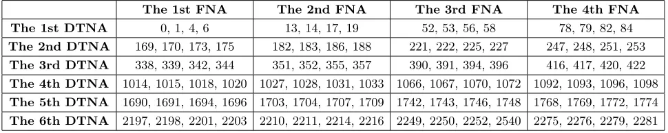
Table 1. Positions of a 96-element TTNA (M = 4,N = 4,H = 6).

The 1st FNA The 2nd FNA The 3rd FNA The 4th FNA

The 1st DTNA 0, 1, 4, 6 13, 14, 17, 19 52, 53, 56, 58 78, 79, 82, 84

The 2nd DTNA 169, 170, 173, 175 182, 183, 186, 188 221, 222, 225, 227 247, 248, 251, 253 The 3rd DTNA 338, 339, 342, 344 351, 352, 355, 357 390, 391, 394, 396 416, 417, 420, 422 The 4th DTNA 1014, 1015, 1018, 1020 1027, 1028, 1031, 1033 1066, 1067, 1070, 1072 1092, 1093, 1096, 1098 The 5th DTNA 1690, 1691, 1694, 1696 1703, 1704, 1707, 1709 1742, 1743, 1746, 1748 1768, 1769, 1772, 1774 The 6th DTNA 2197, 2198, 2201, 2203 2210, 2211, 2214, 2216 2249, 2250, 2252, 2540 2275, 2276, 2279, 2281

Here we consider that the FNA consists of anM1-element uniform array and anM2-element sparse array, whereM1+M2 = M. The LNA consists of an N1-element large-interval uniform array and an

N2-element large-interval sparse array, whereN1+N2 =N. The SLNA consists of anH1-element super large-interval uniform array and an H2-element superlarge-interval sparse array, where H1+H2 =H. For given M, N, and H, the optimal M1, M2, N1, N2 and H1, H2 can be obtained as [10]. Taking a 96-element TTNA (M = 4, N = 4, H = 6) as example, the positions of this TTNA are depicted in Table 1.

Remark 1: It should be clear that the authors consider the (M1+M2)-element nested array as an (M1−1)-element uniform array,M2-element large-interval uniform array, and an isolated sensor in [10]. We use the new description only for the convenience of expression in the following page. In addition, the DTNA is first proposed by Yang et al. in [14], but the DTNA [14] consists of multiple nested arrays [8]. In [21], the authors have proposed a nested MIMO array, whose equivalent array construction is the same as the DTNA in Fig. 1.

According to the construction of TTNA, the positions of the nth FNA in the hth DTNA are

denoted by

dah_n,m/m= 1,2,· · · , M

(2)

wheredah_n,m is the location of the mth sensor in the nth FNA of thehth DTNA. The expression ofa1_n,m can be given by

a1_n,m=

⎧ ⎪ ⎪ ⎪ ⎪ ⎪ ⎪ ⎪ ⎪ ⎪ ⎪ ⎪ ⎪ ⎪ ⎪ ⎨ ⎪ ⎪ ⎪ ⎪ ⎪ ⎪ ⎪ ⎪ ⎪ ⎪ ⎪ ⎪ ⎪ ⎪ ⎩

(m−1) +D(n−1), when m≤M1, n≤N1

M1m−M12+m−1 +D(n−1), when M1< m < M, n≤N1

M2M1+M−2 +D(n−1), when m=M, n≤N1

(m−1) +D(N1n−N12+n−1), when m≤M1, N1 < n < N

M1m−M12+m−1 +D(N1n−N12+n−1), when M1< m < M, N1< n < N

M2M1+M−2 +D(N1n−N12+n−1), when m=M, N1 < n < N (m−1) +D(N2N1+N−2), when m≤M1, n=N

M1m−M12+m−1 +D(N2N1+N −2), when M1< m < M, n=N

M2M1+M−2 +D(N2N1+N −2), when m=M, n=N

whereD= 2M + 2M2M1−3, then ah_n,m can be expressed as

ah_n,m=

⎧ ⎪ ⎨ ⎪ ⎩

a1_n,m+D1(h−1), when h≤H1

a1_n,m+D1(H1h−H12+h−1), when H1< h < H

a1_n,m+D1(H2H1+H−2), when h=H

(4)

whereD1 is the DOFs of DTNA.

Omitting the symbol of unit inter-element spacingd, we denote the position set of thenth FNA in thehth DTNA as

Lh_n=

ah_n,m/m= 1,2,· · · , M

(5)

From Eqs. (3)–(5), we can know that

Min

Lh_n1

−Max

Lh_n2

>0 (6)

wheren1 > n2.

Denote the nonnegative cross-lap set between then1th FNA and n2th FNA in thehth DTNA as

Lh

n1,n2 which can be expressed as

Lh_n1,n2 =

ah_n1m1−ah_n2m2/m1 = 1,2,· · · , M, m2 = 1,2,· · · , M

, n1 > n2

ah_n1m1−ah_n2m2/m1 = 1,2,· · · , M, m2 = 1,2,· · · , M, m1 ≥m2

, n1 =n2

(7)

Then, the nonnegative self-lap set of thehth DTNA can be described as

Lh=

n1>n2

Lh_n1,n2

Lh_n,n (8)

wheren is an arbitrary integer from 1 toN.

Denote the nonnegative cross-lap set between the h1th DTNA and h2th DTNA as Lh1,h2 which can be expressed as

Lh1,h2 ₌

ah1

n1m1−ahn22m2/m1, m2 = 1,2,· · · , M;n1, n2 = 1,2,· · ·, N

, when h1 > h2

Lh1_{, when h1 =h2} (9)

Then, the nonnegative lap set of TTNA can be described as

L=

⎛

⎝

h1>h2

Lh1,h2

⎞

⎠_Lh ₍₁₀₎

whereh is an arbitrary integer from 1 to H.

In order to get the DOFs of the proposed TTNA and drive the detailed process for constructing covariance matrix, we generalize the properties ofLh_n1,n2,Lh and L, which can be listed as follows.

Proposition 1: As n1> n2, following descriptions hold for the cross-lap set Lh_n1,n2. (a)Lh

n1,n2 contains all the contiguous integers from Min{Lhn1,n2} to Max{Lhn1,n2}.

(b)Lh_n1,n2= 2M + 2M2M1−3 =D. The proof can be found in Appendix A.

Proposition 2: Lhcontains all the contiguous integers from Min{Lh}to Max{Lh}, where Min{Lh}= 0 and Max{Lh}= [N +N1N2−2][2M −3 + 2M2M1] +M+M2M1−2.

The proof can be found in Appendix B.

Proposition 3: L contains all the contiguous integers from Min{L} to Max{L}, where Min{L} = 0 and Max{L}= (D1−1)/2 +D1(H+H2H1−2), where D1= [2N + 2N1N2−3][2M + 2M2M1−3].

The proof can be found in Appendix C.

According to Proposition 3 and the symmetry of laps, we can know that the negative lap set L−

Table 2. DOFs of three multiple-nested array configurations. Number of

sensors Proposed TTNA DTNA DTNA [14]

64 2197 (M = 4, N = 4, H= 4) 2025 (M = 8,N = 8) 1521 (M = 8,N = 8) 80 3211 (M = 4, N = 4, H= 5) 3015 (M = 8,N = 10) 2301 (M = 8,N = 10) 96 4563 (M = 4, N = 4, H= 6) 4185 (M = 8,N = 12) 3237 (M = 8,N = 12) 100 4693 (M = 4, N = 5, H= 5) 4489 (M = 10,N = 10) 3481 (M = 10,N = 10) 112 5915 (M = 4, N = 4, H= 7) 5915 (M = 8,N = 14) 4329 (M = 8,N = 14) 120 6669 (M = 4, N = 5, H= 6) 6231 (M = 10,N = 12) 4897 (M = 10,N = 12) 125 6859 (M = 5, N = 5, H= 5) 6821 (M = 5,N = 25) 5729 (M = 5,N = 25) 150 9747 (M = 5, N = 5, H= 6) 9313 (M = 10,N = 15) 7493 (M = 10,N = 15)

obtain that the DOFs of TTNA areD1(2H+ 2H2H1−3). Table 2 shows the DOFs of three multiple-nested arrays under different numbers of sensors. From Table 2, we can see clearly that the proposed multiple-nested array can provide more DOFs than DTNA [14] and DTNA.

Remark 2: We must notice that the number of sensors in nested array [10] is no less than 4. Hence, the number of sensors in proposed TTNA should be written as the product of three integers greater than 4. Just for this case, we only give the expression of DOFs on certain number of sensors, such as 64, 80, and 96. When the number of sensors is smaller than 64, we can see the DTNA as the particular TTNA with H= 1. DOFs of five nested arrays with small number of sensors are listed in Table 3.

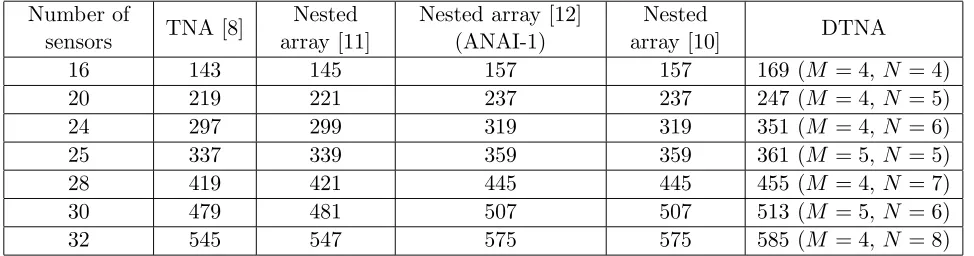
Table 3. DOFs of five nested array configurations. Number of

sensors TNA [8]

Nested array [11]

Nested array [12] (ANAI-1)

Nested

array [10] DTNA

16 143 145 157 157 169 (M = 4, N = 4)

20 219 221 237 237 247 (M = 4, N = 5)

24 297 299 319 319 351 (M = 4, N = 6)

25 337 339 359 359 361 (M = 5, N = 5)

28 419 421 445 445 455 (M = 4, N = 7)

30 479 481 507 507 513 (M = 5, N = 6)

32 545 547 575 575 585 (M = 4, N = 8)

4. CONSTRUCTION OF EXTENDED COVARIANCE MATRIX

Constructing extended covariance matrix is the key point to increase the potential DOFs of a sparse array. Spatial smoothing (SS) [23, 24] is a well-known technique to construct an extended full-rank covariance matrix. The principle of SS algorithm is briefly introduced as follows.

Denote the conventional covariance matrix R_xx = E{xxH¯_{}, where x is the received data vector} described in Eq. (1). Then we can obtain a vector z = vec(R_xx). Picking out all the consecutive lags samples ofz, then we can construct a new vectorznew. Suppose that the length ofznew is 2Lε+ 1, and two kinds of extended covariance matrix can be constructed as [23, 24], respectively

R_xx = 1

Lε+ 1 Lε+1

i=1

znew(Lε+ 2−i: 2Lε+ 2−i)zHnew(Lε+ 2−i: 2Lε+ 2−i)) (11) or

where znew(Lε+ 2−i: 2Lε+ 2−i) stands for a vector composed by the (Lε+ 2−i)th component to the (2Lε+ 2−i)th component of znew.

Performing EVD of R_xx or R_xx, the DOA can be estimated by the MUSIC [25] or ESPRIT algorithm [26].

In fact, only Lε+ 1 elements are exploited to form the vector znew; therefore, we do not need to obtain all the elements of vector z. Then, we introduce the detailed process for constructing the vector

znew according to the special structure characteristic of proposed TTNA.

Based on Eq. (1), the received data of themth sensor in the nth FNA of the hth DTNA can be expressed as

xh_nm(t) =

e−i2πλdahm,nsin(θ1) _{· · · e}−i2π_λdahm,nsin(θK) _{s(t) +n}h

n,m(t) (13)

We first define the continuous sampling covariance vector betweenxh1

n1 andxhn22 asznh11,h,n22, wherexhn11

andxh2

n2 are the data vector of then1th FNA of theh1th DTNA and then2th FNA of theh2th DTNA,

respectively. Whenxh1

n1 =xhn22 =xhn,zh,hn,n can be expressed as

zh,h_n,n =

E{xh_n,M1(xh_n,M1)∗}, E{xh_n,M1(xh_n,M1−1)∗},· · · , E{xhn,M1(xhn,1)∗}, E{xhn,M(xhn,M−1)∗}

E{xh_n,M1+1(xhn,M1)∗}, E{xhn,M1+1(xhn,M1−1)∗},· · · , E{xhn,M1+1(xhn,1)∗}, E{xhn,M(xhn,M−2)∗} ..

.

E{xh_n,M−1(xhn,M1)∗}, E{xhn,M−1(xhn,M1−1)∗},· · · , E{xhn,M−1(xhn,1)∗}, E{xhn,M(xhn,M1)∗}

E{xh_n,M(xh_n,M1−1)∗}, E{xhn,M(xhn,M1−2)∗},· · ·, E{xhn,M(xhn,1)∗}

_T

∈C(M+M1M2−1)×1 ₍₁₄₎

Whenxh1

n1 =xhn22, we denotezhn11,h,n22=[ (z1hn1,h1,n22)T (z

h1,h2

2n1,n2)T (z

h1,h2

3n1,n2)T (z

h1,h2

4n1,n2)T (z

h1,h2

5n1,n2)T ]T,

wherezh_1n1,h_1,n2₂,zh_2n1,h_1,n2₂,z₃h_n1₁,h_,n2₂,z₄h_n1₁,h_,n2₂ and z₅h_n1,h_1,n2₂ can be expressed as

zh_1n1,h_1,n2₂ =

E{xh_n1_1,1(xnh22,M)∗}, E{xnh11,2(xhn22,M)∗},· · ·, E{xhn11,M1(x

h2

n2,M)∗}, E{xhn11,1(xhn22,M−1)∗},

E{xh_n1_1,2(xhn22,M−1)∗},· · · , E{xhn11,M1(x

h2

n2,M−1)∗}

_T

∈C2M1×1 (15)

zh_2n1,h2 1,n2 =

E{xh1

n1,M1+1(xnh22,M)∗}, E{xhn11,1(x_nh2_2,M−2)∗}, E{xhn11,2(xh_n2_2,M−2)∗},· · · , E{xhn11,M1(x

h2

n2,M−2)∗},

E{xh_n1_1,M1+2(xhn22,M)∗}, E{xhn11,1(xh_n2_2,M−3)∗}, E{xhn11,2(xh_n2_2,M−3)∗},· · · , E{xhn11,M1(x

h2

n2,M−3)∗}, ..

.

E{xh_n1_1,M−2(xhn22,M)∗}, E{xhn11,1(xhn22,M1+1)∗}, E{xhn11,2(xhn22,M1+1)∗},· · · , E{xhn11,M1(x

h2

n2,M1+1)∗},

E{xh_n1_1,M−1(xhn22,M)∗}

_T

∈C[(M2−2)M1+M2−1]×1 ₍₁₆₎

zh_3n1,h2 1,n2 =

E{xh1

n1,1(xh_n2_2,M1)∗}, E{xnh11,2(xh_n2_2,M1)∗},· · ·, E{x_nh1_1,M1(xh_n2_2,M1)∗}, E{x_nh1_1,M1(xh_n2_2,M1−1)∗},

E{xh_n1_1,M1(xh_n2_2,M1−2)∗},· · · , E{xhn11,M1(x

h2

n2,1)∗}

_T

zh_4n1,h2 1n2 =

E{xh1

n1,M(xnh22,M−1)∗}, E{xnh11,M1+1(xnh22,M1)∗}, E{x

h1

n1,M1+1(xnh22,M1−1)∗},

· · ·, E{xh1

n1,M1+1(xhn22,1)∗}, E{xh_n1_1,M(x_nh2_2,M−2)∗}, E{xnh11,M1+2(xhn22,M1)},

E{xh1

n1,M1+2(xnh22,M1−1)},· · · , E{xhn11,M1+2(xhn22,1)}, .. .

E{xh_n1_1,M(xh_n2_2,M1+2)∗}, E{xhn11,M−2(xhn22,M1)

∗_{}, E{x}h1

n1,M−2(xnh22,M1−1)∗},

· · ·, E{xh_n1_1,M−2(xhn22,1)∗}, E{xh_n1_1,M(x_nh2_2,M1+1)∗}

_T

∈C[(M2−2)M1+M2−1]×1 (18)

zh_5n1,h_1n2₂ =

E{xh_n1_1,M−1(xhn22,M1)

∗_{}, E{x}h1

n1,M−1(xhn22,M1−1)∗},· · ·, E{xnh11,M−1(xnh22,1)∗},

E{xh_n1_1,M(xh_n2_2,M1)∗}, E{xh_n1_1,M(x_nh2_2,M1−1)∗},· · ·, E{xnh11,M(xhn22,1)∗}

_T

∈C2M1×1 (19)

Then, we denote zh1,h2 _{as continuous lap sampling covariance vector between x}h1 _{and x}h2_{, where} xh1 _{and x}h2 _{are the data vector of the h1th DTNA andh2th DTNA, respectively.}

Whenxh1 _=xh2 _=xh_{, z}h,h _{can be expressed as}

zh,h =

(zh,h_N 1,N1)

T_,(zh,h

N1,N1−1)T,(zh,hN1,N1−2)T,· · ·,(zh,hN1,1)T,(zh,hN,N−1)T (zh,h_N

1+1,N1)

T_,(zh,h

N1+1,N1−1)T,· · · ,(zh,hN1+1,1)T,(zh,hN,N−2)T, ..

. (zh,h_N−1,N

1)T,(z

h,h

N−1,N1−1)T,· · · ,(z h,h

N−1,1)T,(z h,h N,N1)T

(zh,h_N,N

1−1)T,(zh,hN,N1−2)T,· · ·,(zh,hN,1)T

_T

(20)

When xh1 _{= x}h2_{, we denote z}h1,h2 _{= [ (z}h1,h2

1 )T (zh21,h2)T (zh31,h2)T (z4h1,h2)T (z5h1,h2)T ]T, wherezh₁1,h2,z₂h1,h2,z₃h1,h2,zh₄1,h2 andzh₅1,h2 can be expressed as

zh₁1,h2=

zh_1,N1,h2

_T

,

zh_2,N1,h2

_T

,· · ·,

zh_N1₁,h_,N2

_T

,

zh_1,N1,h₋2₁

_T

,

zh_2,N1,h₋2₁

_T

,· · · ,

zh_N1₁,h_,N2₋₁

_TT

(21)

zh₂1,h2= zh_N1,h2 1+1,N

_T

,

zh_1,N1,h₋2₂

_T

,

zh_2,N1,h₋2₂

_T

,· · · ,

zh_N1,h2 1,N−2

_T

,

zh_N1,h2 1+2,N

_T

,

zh_1,N1,h₋2₃

_T

,

zh_2,N1,h₋2₃

_T

,· · ·,

zh_N1,h2 1,N−3

_T

,

.. .

zh_N1₋,h₂2_,N

_T

,

zh_1,N1,h₁2₊₁

_T

,

zh_2,N1,h₁2₊₁

_T

,· · ·,

zh_N1₁,h_,N2₁₊₁

_T

,

zh_N1₋,h₁2_,N

_TT

(22)

zh₃1,h2=

zh_1,N1,h2 1

_T

,

zh_2,N1,h2 1

_T

,· · ·,

zh_N1,h2 1,N1

_T

,

zh_N1,h2 1,N1−1

_T

,

zh_N1,h2 1,N1−2

_T

,· · · ,

zh_N1,h2 1,1

_TT

(23)

zh₄1,h2= zh_N,N1,h2₋₁

_T

,

zh_N1₁,h₊₁2_,N1

_T

,

zh_N1₁,h₊₁2_,N1−1

_T

,· · · ,

zh_N1₁,h₊₁2_,1

_T

zh_N,N1,h2₋₂,zh_N1,h2 1+2,N1

_T

,

zh_N1,h2 1+2,N1−1

_T

,· · · ,

zh_N1,h2 1+2,1

_T

.. .

zh_N,N1,h2 1+2

_T

,

zh_N1₋,h₂2_,N 1

_T

,

zh_N1₋,h₂2_,N 1−1

_T

,· · ·,

zh_N1₋,h₂2_,1

_T

,

zh_N,N1,h2 1+1

_T T

(24)

zh₅1,h2=

zh_N1₋,h₁2_,N 1

_T

,

zh_N1₋,h₁2_,N 1−1

_T

,· · · ,

zh_N1₋,h₁2_,1

_T

,

zh_N,N1,h2 1

_T

,

zh_N,N1,h2 1−1

_T

,· · · ,

zh_N,1,h₁2

_TT

(25)

Then we can construct a vector as

z+ =

(zH1,H1)T,(zH1,H1−1)T,(zH1,H1−2)T,· · · ,(zH1,1)T,(zH,H−1)T (zH1+1,H1₎T_,(zH1+1,H1−1₎T_{,· · · ,(z}H1+1,1₎T_,(zH,H−2₎T_,

.. .

(zH−1,H1₎T_,(zH−1,H1−1₎T_{,· · ·,(z}H−1,1₎T_,(zH,H1₎T_, (zH,H1−1₎T_,(zH,H1−2₎T_{,· · ·,(z}H,1₎T

_T

(26)

According to the proofs of Appendix A, Appendix B, and Appendix C, we know thatz+ consists of all the non-negative consecutive lap samples. According to the symmetry of lap, we can obtain znew as

znew=

Jz∗₊2 : DOFs+1₂

z+

(27)

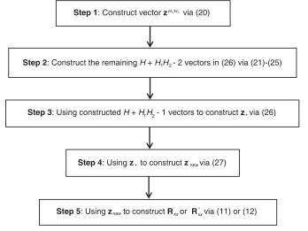
According to Eqs. (11) and (12), we can obtain the extended covariance matrix R_xx or R_xx. The flowchart about constructing the covariance matrix is shown in Fig. 2.

Step 1: Construct vector z H H1 1 via (20)

Step 2: Construct the remaining H + H H1 2- 2 vectorsin (26) via (21)-(25)

Step 3: Using constructed H + H H - 1 vectors to construct z via (26)

new

+

1 2

Step 4: Using z + to construct z via (27)

xx

Step 5: Using z to construct R or R xxvia (11) or (12)

' ''

new

Figure 2. Flowchart of the process to construct covariance matrix.

Figure 3. MUSIC spectra of proposed TTNA for 81 signals.

5. SIMULATION

In this section, we present some experiments to examine the effectiveness of proposed TTNA for DOA estimation. For all nested arrays in each experiment, MUSIC algorithm [25] is used to perform DOA estimation.

5.1. Comparison of Space Spectra

Firstly, we compare the space spectra of three multiple-nested arrays for larger number of sensors. We suppose that the total number of sensors is 64, and SNR is 0 dB. 200 snapshots are used to estimate the extended covariance matrix. The searching range of MUSIC algorithm is from−90◦ to 90◦ with the grid of 0.1◦. Fig. 3, Fig. 4, and Fig. 5 show the MUSIC spectra of three arrays for 81 signals distributed uniformly from−80◦ to 80◦. From Fig. 3, we can find that the proposed TTNA can distinguish the 81 signals clearly. From Fig. 4 and Fig. 5, we can see clearly that a few signals cannot be discriminated by

the other two DTNAs.

Secondly, we compare the space spectra of different nested arrays for smaller number of sensors. Suppose that the total number of sensors is 20, and SNR is 0 dB. 500 snapshots are used to estimate the extended covariance matrix. Because the number of sensors for the common TTNA should be larger than 64, we take a 20-element DTNA as a particular TTNA with H = 1. In [21], some comparison experiments of two equivalent DTNAs with smaller number of sensors have been presented. Hence, we only compare the space spectra of DTNA with other three nested arrays [8, 10, 11]. Fig. 6 shows the MUSIC spectra of 15 signals distributed uniformly between −35◦ and 35◦. Fig. 7 shows the MUSIC spectra of 41 signals distributed uniformly from−80◦ to 80◦. From Fig. 6 and Fig. 7, we can find that DTNA shows higher resolution than the other three nested arrays.

Figure 5. MUSIC spectra of DTNA [14] for 81 signals.

Figure 7. MUSIC spectra of four nested arrays for 41 signals.

5.2. Comparison of RMSE

The root-mean-square error (RMSE) of DOA estimation as the performance measurement is given by

RMSE =

1

KJ

J

j=1 K

k=1

(ˆθkj−θk)2 (28)

whereJ = 200, and ˆθkj is the estimation ofθk in thejth Monte Carlo trial.

Firstly, we compare the RMSE of DOA estimation for three multiple-nested arrays with larger number of sensors. We suppose that the total number of sensors is 64 for the three multiple-nested arrays. Suppose that 41 signals are uniformly distributed from−80◦ to 80◦. Fig. 8 shows the RMSE of DOA estimation versus SNR withT = 200. From Fig. 8, we can see clearly that the RMSE of MUSIC

algorithm with the proposed TTNA is far lower than the other two DTNAs, particularly when the SNR is larger than 0 dB.

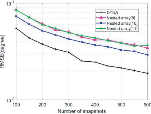
Secondly, we compare the RMSE of DOA estimation for different nested arrays with smaller number of sensors. We suppose that the total number of sensors is 20 for the four nested arrays. The used 20-element DTNA is composed by 4 5-element nested arrays. Suppose that 15 signals are uniformly distributed from −70◦ to −70◦. Fix the snapshots at T = 500, and Fig. 9 shows the RMSE of MUSIC algorithm versus SNR for four nested arrays. Then, we fix SNR at 5 dB, and Fig. 10 shows the RMSE of MUSIC algorithm versus snapshots for four nested arrays. From the two figures, it is clear to find that the RMSE of MUSIC algorithm with the DTNA is lower than the other three nested arrays.

Figure 9. RMSE against SNR for four nested arrays.

6. CONCLUSION

In this paper, we present a new hole-free nested array which consists of multiple fundamental nested arrays. The positions of these fundamental nested arrays are obtained according to the other given nested array. The closed-form expression of DOFs and the detailed process for the construction of extended covariance matrix are given. Compared with many preexisting nested arrays, the proposed nested array can provide more degrees of freedom (DOFs). Because of the increase of DOFs, the proposed array shows higher resolution in DOA estimation. Lots of simulation results certify that the proposed array has better performance for DOA estimation.

APPENDIX A.

Proof of Proposition 1

Observing the setLh_n1,n2, we can find that many repeating elements appear in the set. If we want to know the characteristic of the setLh_n1,n2, we only need to pick out all unique elements. Giving enough thought to the construction of FNA, we denote five sub-sets of Lh_n1,n2 as

Lh1n1n2 = {ahn1,1−ahn2,M, ahn1,2−ahn2,M,· · ·, ahn1,M1−ahn2,M, ahn1,1−ahn2,M−1,

ah_n1,2−ahn2,M−1,· · · , ahn1,M1 −ahn2,M−1} (A1)

Lh2n1n2 = {ahn1,M1+1−ahn2,M, ahn1,1−ahn2,M−2, ahn1,2−ahn2,M−2,· · · , ahn1,M1−ahn2,M−2,

ah_n1,M1+2−ahn2,M, an1,1−ah_n2,M−3, anh1,2−ahn2,M−3,· · · , ahn1,M1 −ahn2,M−3, ..

.

ah_n1,M−2−anh2,M, ahn1,1−anh2,M1+1, ahn1,2−ahn2,M1+1,· · · ,

ah_n1,M1 −ah_n2,M1+1, ahn1,M−1−ahn2,M} (A2)

Lh3n1n2 = {ahn1,1−ahn2,M1, ahn1,2−ahn2,M1,· · ·, ahn1,M1−ahn2,M1, ahn1,M1−ahn2,M1−1,

ah_n1,M1 −ah_n2,M1−2,· · ·, ahn1,M1 −ahn2,1} (A3)

Lh4n1n2 = {ahn1,M−anh2,M−1, ahn1,M1+1−ahn2,M1, ahn1,M1+1−ahn2,M1−1,· · ·, ahn1,M1+1−ahn2,1,

ah_n1,M−ah_n2,M−2, anh1,M1+2−ahn2,M1, ahn1,M1+2−ahn2,M1−1,· · · , ahn1,M1+2−ahn2,1, ..

.

ah_n1,M−ah_n2,M1+2, ahn1,M−2−anh2,M1, ahn1,M−2−ahn2,M1−1,· · · ,

ah_n1,M−2−ahn2,1, ahn1,M−ahn2,M1+1} (A4)

Lh5n1n2 = {ahn1,M−1−ahn2,M1, ahn1,M−1−ahn2,M1−1,· · ·, ahn1,M−1−anh2,1, ahn1,M−ahn2,M1,

ah_n1,M−ah_n2,M1−1,· · · , ahn1,M−ahn2,1} (A5)

According to the rule of the five subsets from Eqs. (A1)–(A5), we have

⎧ ⎪ ⎨ ⎪ ⎩

_Lh

1n1n2=Lh5n1n2= 2M1

_Lh

2n1n2=Lh4n1n2= (M2−2)M1+M2−1

_Lh

3n1n2= 2M1−1

(A6)

ofLh_in1n2. Comparing the last element ofLh_in1n2 with the first element ofLh(i+1)n1n2,i= 1, 2, 3, 4, yields ⎧ ⎪ ⎪ ⎪ ⎪ ⎨ ⎪ ⎪ ⎪ ⎪ ⎩ ah

n1,M1 −ahn2,M−1< ahn1,M1+1−ahn2,M

ah_n1,M−1−ahn2,M < ahn1,1−ahn2,M1

ah_n1,M1 −ah_n2,1 < ah_n1,M−ah_n2,M−1

ah_n1,M −ah_n2,M1+1< ahn1,M−1−ahn2,M1

(A7)

Combining the progressive increase of Lh_in1n2 with Eq. (A7), we can know that any two elements

in 5

i=1

Lh_in1n2 are unequal. Then, it is easy to know

Lh_n1,n2≥Lh1n1n2

+Lh2n1n2

+Lh3n1n2

+Lh4n1n2

+Lh5n1n2

= 2M + 2M2M1−3 =D (A8)

Min(Lh_n1,n2) = Min{Lh_n1} −Max{Lh_n2}=ah_n1,1−ahn2,M (A9)

Max(Lh_n1,n2) = Max{Lh_n1} −Min{Lh_n2}=ah_n1,M−ah_n2,1 (A10)

Lh_n1,n2≤Max(Lh_n1,n2)−Min(Lh_n1,n2)+1 = (ah_n1,M−ah_n2,1)−(ahn1,1−ahn2,M)+1 = 2M+2M2M1−3 (A11)

We also need to notice the fact that equality in Eq. (A8) holds if and only ifLh_n1,n2 contains all the contiguous integers from Min(Lh

n1,n2) to Max(Lhn1,n2).

Combining Eq. (A8) with Eq. (A11), we have

Lh_n1,n2= 2M+ 2M2M1−3 = Max(Lh_n1,n2)−Min(Lh_n1,n2) + 1 (A12)

Then, we can prove the two facts in Proposition 1 simultaneously.

APPENDIX B.

Proof of Proposition 2

ConsiderN2+ 1 groups of cross-lap sets, which are expressed as

⎧ ⎪ ⎪ ⎪ ⎪ ⎪ ⎪ ⎪ ⎨ ⎪ ⎪ ⎪ ⎪ ⎪ ⎪ ⎪ ⎩

Group 1: Lh_N1,N1, Lh_N1,N1−1,· · · , LhN1,1, LhN,N−1

Group 2 : Lh_N1+1,N1, LhN1+1,N1−1,· · · , LhN1+1,1, LhN,N−2 ..

.

Group N2 : Lh_N−1,N1, LhN−1,N1−1,· · · , LhN−1,1, LhN,N1 Group N2+ 1 : Lh_N,N1−1, LhN,N1−2,· · ·, LhN,1

(B1)

Obviously, the last group containsN1−1 sets, and there are N1+ 1 sets in any other group. Hence, it is easy to know that the total number of sets in theN2+ 1 groups is N+N1N2−1.

Because similar rules exist in the top N2 groups, we first consider these groups. In each group, comparing the maximum values of adjacent sets via Eqs. (3), (4), and (7) yields

Max(Lh_n1,n2−1)−Max(Lh_n1,n2) =

Max(Lh_n1)−Min(Lh_n2−1)

−Max(Lh_n1)−Min(Lh_n2)

= Min(Lh_n2)−Min(Lh_n2−1) =D (B2)

whereN −1≥n1 ≥N1, 2≤n2 ≤N1, and

Max(Lh_N,n2)−Max(Lh_N+N1−1−n2,1) =

Max(Lh_N)−Min(Lh_n2)

−Max(Lh_N+N1−1−n2)−Min(L

h 1)

= D (B3)

Then, we consider the N−1 sets Lh_N,N−1,Lh_N,N−2, · · ·,Lh_N,1. Comparing the maximum values of adjacent sets, we have

Max(Lh_N,n2)−Max(Lh_N,n2+1) =

Max(Lh_N)−Min(Lh_n2)

−Max(Lh_N)−Min(Lh_n2+1)

= Min(Lh_n2+1)−Min(Lhn2) =

D, N1−1≥n2 ≥1

(N1+1)D, N1 ≤n2 ≤N−2 (B4) From Eqs. (B2), (B3), and the first case of Eq. (B4), we can confirm that the maximum of each set in the same group grows uniformly withD being common difference.

Next, we consider all the sets in the N2+ 1 groups and sort them based on the order in Eq. (B1). For example, we call Lh_N,N−1 as the (N1+ 1)th set, and LhN1+1,N1 as the (N1+ 2)th set. According to

the second case of Eq. (B4), we can further confirm that theN+N1N2−1 maximums of corresponding

N +N1N2−1 sets increase with Dbeing common difference. Based on Proposition 1, Lh_n1,n2 contains all the contiguous integers from Min(Lh_n1,n2) to Max(Lh_n1,n2) and Lh_n1,n2 = D when n1 > n2. It is indicated that Max{Lh_n1,n2} −Min{Lh_n1,n2}=D−1. Then, it is easy to know that the minimum of the

ith set is one more than the maximum of (i−1)th set whenN+N1N2−1≥i >1. Denote the union of the N+N1N2−1 sets in Eq. (B1) as

¯

Lh =

⎛

⎝n1=N−1, n2=N1

n1=N1,n2=1

Lh_{n1, n2} ⎞

⎠

_N−1

n2=1

Lh_{N, n2}

. (B5)

It is clear that ¯Lh contains all the contiguous integers from Min(Lh_N1,N1) to Max(Lh_N,1). Because Min(Lh_N1,N1) = Min(Lh), Max(Lh_N,1) = Max(Lh) and ¯Lh ⊂ Lh, we know that Lh contains all the contiguous integers from Min(Lh) to Max(Lh_N,1). Since Min(Lh) = 0 and Max(Lh) = [N +N1N2 − 2][2M + 2M2M1 −3] +M +M2M1−2, L contains all the integers from 0 to [N +N1N2−2][2M + 2M2M1−3] +M+M2M1−2.

APPENDIX C.

Proof of Proposition 3

Denoting the position set of the hth DTNA as Ph_={Lh

1, Lh2,· · ·, LhN}, the number of integers between Max(Ph) and Max(Ph+1) can be expressed as

Wh,h+1=

⎧ ⎨ ⎩

D1−1, when 1≤h≤H1−1 (H1+ 1)D1−1, when H1≤h < H−1

H1D1−1, when h=H−1

(C1)

Denoting Lhn11,h,n22 as non-negative cross-lap set between Lhn11 and Lhn22, it is easy to know that the

non-negative cross-lapset Lh1,h2_{(h1 > h2) can be seen as the union of some differentL}h1,h2

n1,n2.

As proposition 1, consideringLh1, Lh2,· · · , Lh_N asN numbers, we can find that the number of different

Lhn11,h,n22 is 2N + 2N2N1 −3, and the intersection of any two different Lhn11,h,n22 is empty. According to

Eq. (A12), we can know thatLhn11,n,h22=2M + 2M2M1−3, so we have

Lh1,h2_{= (2M+ 2M}

2M1−3)(2N + 2N2N1−3) =D1, (h1> h2) (C2)

After computing Max(Ph) and Max(Ph+1), we can drive that

1) Lh+1,1 contains all the integers between Max(Ph) and Max(Ph+1), when 1≤h≤H1−1;

2) TheH1+1 setsLh+1,H1,Lh+1,H1−1,· · ·,Lh+1,1andLH,H−(h−H1+1)contain all the integers between Max(Ph) and Max(Ph+1), whenH1 ≤h < H−1;

3) TheH1 sets LH,H1,LH,H1−1,· · ·,LH,1 contain all the integers between Max(Ph) and Max(Ph+1), whenH1 ≤h≤H−1.

ACKNOWLEDGMENT

This work was supported by the National Natural Science Foundation of China (51877015, 51877179), the Cooperation Agreement Foundation by the Department of Science and Technology of Guizhou Province of China (LH[2017]7320, LH[2017]7321), the Innovation Group Major Research Program Funded by Guizhou Provincial Education Department (KY [2016] 051), the Foundation of Top-notch Talents by Education Department of Guizhou Province of China (KY [2018]075) and PhD Research Startup Foundation of Tongren University (trxyDH1710).

REFERENCES

1. Moffet, A., “Minimum-redundancy linear arrays,” IEEE Transactions on Antennas and Propagation, Vol. 16, No. 2, 172–175, 1968.

2. Vaidyanathan, P. P. and P. Pal, “Sparse sensing with co-prime samplers and arrays,” IEEE Transactions on Signal Processing, Vol. 59, No. 2, 573–586, 2011.

3. Qin, S., Y. D. Zhang, and M. G. Amin, “Generalized coprime array configurations for direction-of-arrival estimation,”IEEE Transactions on Signal Processing, Vol. 63, No. 6, 1377–1390, 2015. 4. Ren, S. W., W. J. Wang, and Z. H. Chen, “DOA estimation exploiting unified coprime array with

multi-period subarrays,” 2016 CIE International Conference on Radar (RADAR), Guangzhou, China, 2016.

5. Chen, M., L. Gan, and W. Wang, “Co-prime arrays with reduced sensors (CARS) for direction-of-arrival estimation,” 2017 Sensor Signal Processing for Defence Conference (SSPD), London, UK, 2017.

6. Shi, J., G. Hu, X. Zhang, and Y. Xiao, “Symmetric sum coarray based co-prime MIMO configuration for direction of arrival estimation,” AEU — International Journal of Electronics and Communications, Vol. 94, 339–347, 2018.

7. Shi, J., G. Hu, and X. Zhang, “Generalized co-prime MIMO radar for DOA estimation with enhanced degrees of freedom,” IEEE Sensors Journal, Vol. 18, No. 3, 1203–1212, 2018.

8. Pal, P. and P. P. Vaidyanathan, “Nested arrays: A novel approach to array processing with enhanced degrees of freedom,”IEEE Transactions on Signal Processing, Vol. 58, No. 8, 4167–4181, 2010.

9. Yang, M., A. M. Haimovich, and B. Chen, “A new array geometry for DOA estimation with enhanced degrees of freedom,”2016 IEEE International Conference on Acoustics, Speech and Signal Processing, 3041–3045, Shanghai, China, 2016.

10. Yang, M., L. Sun, X. Yuan, and B. Chen, “Improved nested array with hole-free DCA and more degrees of freedom,”Electron. Lett., Vol. 52, No. 25, 2068–2070, 2016.

11. Iizuka, Y. and K. Ichige, “Extension of nested array for large aperture and high degree of freedom,”IEICE Communications Express, Vol. 6, No. 6, 381–386, 2017.

12. Liu, J., Y. Zhang, Y. Lu, S. Ren, and S. Cao, “Augmented nested arrays with enhanced DOF and reduced mutual coupling,” IEEE Transactions on Signal Processing, Vol. 65, No. 21, 5549–5563, 2017.

13. Shi, J., G. Hu, X. Zhang, and H. Zhou, “Generalized nested array: Optimization for degrees of freedom and mutual coupling,”IEEE Communications Letters, Vol. 22, No. 6, 1208–1211, 2018. 14. Yang, M., A. M. Haimovich, and X. Yuan, “A unified array geometry composed of multiple identical

subarrays with hole-free difference coarrays for underdetermined DOA estimation,” IEEE Access, Vol. 6, 14238–14254, 2018.

15. Huang, H., B. Liao, X. Wang, X. Guo, and J. Huang, “A new nested array configuration with increased degrees of freedom,”IEEE Access, Vol. 6, 1490–1497, 2018.

16. Liu, S., J. Zhao, D. Wu, and H. Cao, “Grade nested array with increased degrees of freedom for quasi-stationary signals,” Progress In Electromagnetics Research Letters, Vol. 80, 75–82, 2018. 17. Liu, S., L. Yang, and D. Li, “Subspace extension algorithm for 2D DOAestimation with L-shaped

18. Ahmed, A., Y. D. Zhang, and B. Himed, “Effective nested array design for fourth-order cumulant-based DOA estimation,” IEEE Radar Conference, 0998–1002, Seattle, WA, USA, 2017.

19. Zhang, L., S. Ren, and X. Li, “Generalized L-shaped nested array concept based on the fourth-order difference co-array,” Sensors, Vol. 18, 8, 2018.

20. Yang, M., L. Sun, X. Yuan, and B. Chen, “A new nested MIMO array with increased degrees of freedom and hole-free difference coarray,” IEEE Signal Processing Letters, Vol. 25, No. 1, 40–44, 2018.

21. Liu, Q., B. Wang, X. Li, J. Tian, T. Cheng, and S. Liu, “An optimizing nested MIMO array with hole-free difference coarray,” MATEC Web of Conferences, Vol. 232, EDP Sciences, 2018.

22. Morabito, A. F. and P. G. Nicolaci, “Optimal synthesis of shaped beams through concentric ring isophoric sparse arrays,”IEEE Antennas and Wireless Propagation Letters, Vol. 16, 979–982, 2017. 23. Pal, P. and P. P. Vaidyanathan, “Coprime sampling and the MUSIC algorithm,” Proceedings of Digital Signal Processing Workshop and IEEE Signal Processing Education Workshop (DSP/SPE), 289–294, Sedona, AZ, USA, 2011.

24. Gu, J. F., P. Wei, and H. M. Tai, “2-D direction-of-arrival estimation of coherent signals using cross-correlation matrix,” Signal Processing, Vol. 88, 75–85, 2008.

25. Schmidt, R. O., “Multiple emitter location and signal parameter estimation,” IEEE Transactions on Antennas and Propagation, Vol. 34, No. 3, 276–280, 1986.