Identifying Large-Scale RFID Tags Using Non-Cryptographic
Approach
Yalin Chen 1, Jue-Sam Chou 2, Cheng-Lun Wu 3, Chi-Fong Lin 4 1
Institute of information systems and applications, National Tsing Hua University, Taiwan
2, 3, 4
Department of Information Management, Nanhua University, Taiwan
[email protected], [email protected], [email protected]
Abstract
In this paper, we propose a new approach to identify a tag of a RFID system in constant time while keeping untraceability to the tag. Our scheme does not use any cryptographic primitives. Instead, we use a line in a plane to represent a tag. The points on the line, which are infinite and different each other, can be used as tag identification. We also explore the scalability of the proposed scheme. The result of experiments showed that a tag of the RFID system over 1,000,000 tags, embedded 3000 gates, can store 559 dynamic identity proofs.
Keywords: radio frequency identification, RFID, identification protocol, privacy,
untraceability, location privacy, scalability
1. Introduction
The Radio Frequency Identification (RFID) technique allows identifying hundreds of objects one time via a contactless manner. It therefore becomes an important role in many applications such as automobile immobilization, RTLS (Real Time Location Systems), baggage handling, animal tracing, and item-level tagging in fashion apparels. However, the RFID technique brings not only new opportunities but also new challenges. In particular, secure and private RFID tag identification protocol is a demanding task since the resource of RFID tags is extremely limited. There are three roles in a typical RFID system: tags which are embedded in objects to be identified,
readers which emit radio signals to interrogate tags, and a server which maintains all tags' information, identifies tags and provides services. In this paper, we focus on three features of the RFID identification protocols.
First, as being a low-cost device, a passive RFID tag is not powered and accommodates only a few hundreds to thousands gates. Traditional cryptographic primitives are thus hardly applied on such cheap tags [1, 2]. In addition, as tags are usually embedded in objects carried by people everywhere, the user location privacy
identity. Meanwhile, a third party cannot link the DID to any particular tag and thus cannot locate the user who carries the tag. Researchers also refer this property as
untraceability or unlinkability. Third, since many RFID applications require deploying the tags in large scale, the scalability is also an important feature. If a server takes linear time to identify a tag, the identification time for the server will increase as the number of tags increase. This will limit the scalability of a RFID system. Conversely, if a server takes constant time to identify a tag, the number of tags will not be limited. Therefore, RFID scalability can be realized as constant-time tag identification.
In recent decades, many secure and private RFID authentication protocol are proposed. Weies et al. [1] proposed a hash-based method to reserves user location privacy. Their scheme uses a random number r and tag's secret key k to make a DID, i.e. h(k, r), where h(.) is a one-way hash function. However, the server has to linearly search its database (DB) to compare whether each h(ki, r) is equal to the received h(k,
r). This limits the scalability. Recent work [6] is a similar approach and suffers the same problem.
Ohkubo, Suzuki and Kinoshita (OSK) [2] proposed another hashed-based method to further assure forward secrecy: even if tag's secrecy is exposed, the past transactions that the tag was involved cannot be linked to the tag. In their scheme, a tag and server share secrecy s0 when initialized. After deployment, on receiving the
ith query, the tag responds with h(si), where si = g(si-1) and g(.) is another one-way
hash function. On seeing h(si), the server reads its DB record by record. Suppose it is reading the jth record and sj* is the corresponding seed. The server will compare whether the received h(si) is equal to h(g1(sj*)), h(g2(sj*)), ..., or h(gm(sj*)), where gm(.) indicates performing function g(.) m times. Consequently, the server has to take O(mN) time for each tag identification, where N refers to number of tags.
Studies [7, 8] arrange tags in a tree structure on secret keys they possess to reduce the identification complexity to O(logN). However scheme [7] will be broken since compromising 20 tags in a system of N=220 tags reveals the identities of other tags. The improved scheme [8] requires updating overhead in O(logN) in order to remedy the problem in [7]. Another major weakness is that the tree-based approach leads high communication overhead between tag and reader. Some researchers believe these drawbacks overweigh the reduction in identification complexity [13].
the worst case, a tag, suffered malicious queries before, will not answer the expected response and the server will therefore launch brute searching for the tag identification. Alomair et al. [13, 14] uses two layers pointers to save pre-built DIDs − h(Ψi, c)s, where Ψi is a pseudonym and c is counter ranging form zero to C − to allows malicious queries to a specific tag at least C times. The size of the first-layer table is estimated as O(NC) and each record point to a second-layer table. The each second-layer table which points to a tag information is expected to contain only one record. As a result, it assure constant-time identification when server seeing h(Ψi, c). After recognizing Ψi, the server assigns an unoccupied pseudonym Ψk to the tag, where h(Ψk, 0), h(Ψk, 1), ..., and h(Ψk, C) in the second-layer tables point to an empty tag record, position p. Finally, the server updates its tables by moving the tag information record to the new position p and emptying the original tag record, say position p', as null. By this way it assures O(1) update.
Ryu and Takagi (RT) [15] stores one-time values ∆={α1, ..., αm} as DIDs on a tag where αi = Epk(TagID||r), Epk(.) is a public key encryption and the corresponding private key only known to the server. For each interrogation, the tag responds with a fresh one-time pad and a reader is allowed to write new one-time values in the tag after successfully mutual authentication. As the server can obtain tag identity by decrypting a received αi, RT achieves constant-time identification and thus assures scalability. However, for about 60-bit security level, the size of αi is about 512 bits in RSA encryption or 400 bits in ElGamal elliptic-curve encryption (ECC). Then, suppose a tag with 3K bytes memory. It can store only 48 RSA-based or 61 ECC-based ciphertexts. This implies the tolerance for malicious query to a tag is only 48 or 61 times.
Studies [16-18] use ECC-based approach while studies [19, 20] use Rabin's cryptosystem, which are public-key based approaches. Public key cryptosystems easily obtain constant-time tag identification but they pay hardware cost at tag side. The most efficient ECC component costs 12.5K gates [21] while 512-bit Rabin's encryption costs about 17K gates [22] or 10K gates [23]. These obviously greatly exceed the cost of hash-like component AES, about 3.4K gates [24].
The remaining of this paper is organized as follows. Section 2 describes the basic idea of the proposed scheme while Section 3 presents the detailed implementation. Performance evaluation and security analyses of the proposed scheme are shown in Section 4 and 5 respectively. Finally, Section 6 gives conclusion and future work.
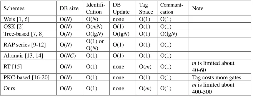
Table 1: Resource usage of the proposed scheme and previous related works
Schemes DB size Identifi- Cation
DB Update
Tag Space
Communi-
cation Note
Weis [1, 6] O(N) O(N) none O(1) O(1) OSK [2] O(N) O(mN) O(1) O(1) O(1) Tree-based [7, 8] O(N) O(lgN) O(lgN) O(1) O(lgN) RAP series [9-12] O(N) O(1) or
O(N) O(1) O(1) O(1) Alomair [13, 14] O(NC) O(1) O(1) O(1) O(1)
RT [15] O(N) O(1) none O(m) O(1) m is limited about 40-60
PKC-based [16-20] O(N) O(1) none O(1) O(1) Tag costs more gates Ours O(N) O(1) none O(m) O(1) m is limited about
400-500
2. Basic Idea
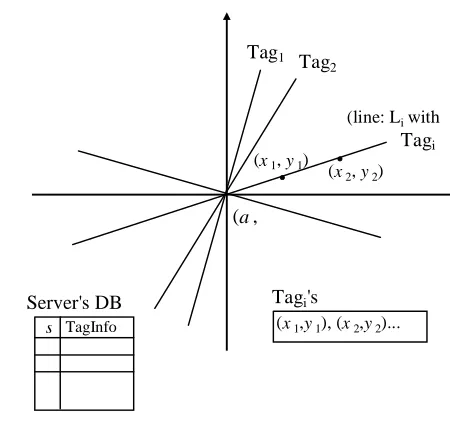
In this work, we would like to use the slope of a line on a plane to represent a tag. The tag then can be identified if it can provide correct information regarding the line. Figure 1 shows the basic idea of our scheme. In the figure, a randomly chosen point (a,
b) is the secrecy of the server. For simplification and without loss of generality, we let
a = b = 0. A line Li having slope si and passing through (a, b) represents tag Ti. Any point (x, y) on the line Li can be a proof of Ti. In addition, we assume that the length of a or b is k-bit long, denoted as |a| = |b| = k. Then, the slopes of lines representing all tags of a RFID system are defined as the set S = {s| s is an integer, −(2k-1−1) s
+(2k-1−1), and s ≠ 0}. Hence, the number of tags in our system is N = 2k − 2. The following algorithm demonstrates the tag initialization of this basic scheme.
Basic Tag Initialization {
S = [-(2k-1
-1), +(2k-1-1)] - {0};
N = |S|; i = 1;
For s = -2k-1+1 to 2k-1-1 { //s presents the slope of a line // setup tag Ti;
for j = 1 to m { // generate m pairs of (x, y) xj R [-(2k-1
-1), +(2k-1-1)] - {a}; yj = s * xj + (b - a * s);
}
Insert {s, TagInfo, x1, x2, ..., xm} into server's database; Next i;
} }
Tag1 Tag 2
Tagi
(a,
b)
(x2, y2)
.
(line: Li with
slop:s)
Tagi's
(x1,y1), (x2,y2)...
Server's DB
s TagInfo
.
(x1, y1)Fig. 1. Basic model of the study
When the tag initialization completed, each tag storage has m tuples of proofs, (x1, y1),
(x2, y2), ..., and (xm, ym). In the identification phase, on receiving an interrogation from a server, a tag will answer an unused (xj, yj) pair. On receiving the pair, the server will compute s = (xj − a)/(yj − b) and then use s to look up the corresponding tag in its DB.
We take k = 8 as an example. Then according to our design, S is a set of all integers in [−127, 127] − {0} and each element in S represents an identity of a tag. Moreover, we let a random pair (a, b) = (−23, −94) be the secret point of the server. Then, we have y = −127x + 2827 to represent a tag which identity is −127 and points (−27, 414), (99, −1558) and (−52, 3589) are the proofs of the tag. When the tag provides any one of these proofs, say (−27, 414), the server can compute the expression s = (414 − (−94))/ (−27 − (−23)) = −127 and thus obtain the identity of the tag.
Our approach has several merits: First, it assures constant-time tag lookup at server side since a server can compute the slope of a tag and then directly fetch the tag record. Furthermore, the constant-time tag identification implies scalability of a RFID system compared to O(N)-time tag identification of many hash-based schemes [1, 2, 6, 9-12] (also see Table 1). The second merit of our approach is that it requires only O(N) space to store tag information at server side. Thirdly, any two observed proofs, which may come from one tag or from two different tags, are indistinguishable. This assures
cryptographic component such as PRNG, Hash or AES. Moreover, when being identified, the tag as long as selects an unused proof as its answer. This takes extremely low computational overhead.
However, some details should be further considered. First, the plaintext of point (x,
y) is not suitable for transmission over an open network since any two eavesdropped pairs (x1, y1) and (x2, y2) from a tag can deduce the slope of the tag. Therefore, (x, y)
pair should be transmitted in an encrypted form. Our countermeasure is that the server transforms a (x, y) into a random-looking string in the initialization phase. Thus, the random-looking result will play as a one-time pad and hence achieve unconditional security. That is, even an adversary intends to exhaustively guess the server's secret point (a, b), he does not has any clue − the plain (x, y)s or slopes − to examine his guess. Second, the tag's memory size will be a limitation. As x and s both are k-bit long integers, the value of the y will be about 2k-bit long. If a tag stores such a (x, y) pair in a plain manner, it would take 3k bits. For example, supposing k is 20 bits, the tag would take 60 bits of storage to store a (x, y) pair. Thus, a tag having 2K-byte storage can store about 273 pairs of (x, y). We consider that if the storage size of the y
can be reduced to 20 bits as same as the storage size of x, the tag then can store over 400 pairs of (x, y). Therefore, the problem of this study can be further formulated as how to downsize the storage of the y values.
3. The Proposed Scheme
In this section, we present a practical implementation based on our basic model. In the implementation, we first consider how to store the y values in tags; i.e. how to encode the y value to attain better space efficiency.
We start the discussion from the range of y values. The maximum of all possible y
for any (a, b), denoted as YMAX, is
YMAX = 2(2k-1−1)2 − 3*2k-1 + 122k-1
when (s, a, b, x) = (2k-1−1,−(2k-1−1),2k-1−1,2k-1−1) or (−(2k-1−1),2k-1−1,2k-1−1,−(2k-1−1)). And y will reach the minimum, denoted as YMIN,
YMIN = −2(2k-1−1)2 + 3*2k-1 − 1−22k-1
when (s, a, b, x)=(−(2k-1−1),−(2k-1−1),−(2k-1−1),2k-1−1)or (2k-1−1,2k-1−1,−(2k-1−1),−(2k-1−1)). Take k as 4 bits for example. The range of x will fall in [−7, 7] while the range of y
will fall in [−105, 105]. YMAX is 105 when (s, a, b, x) = (7, −7, 7, 7) or (−7, 7, 7, −7) while YMIN is −105 when (s, a, b, x) = (−7, −7, −7, 7) or (7, 7, −7, −7). Thus, storing
y value requires about 8 bits while storing x value requires only 4 bits.
and random point (a, b) is equal to (−68, 79), (−127, −127) and (127, 127), respectively.
Fig. 2. Distributions of (x, y) pairs of (a, b) = (-68, 79), (-127, -127) and (127, 127)
From Figure 2, we believe that y value can be compressed through some transformation algorithms and mapped to a smaller space. Our intuitive solution has two phases. Briefly, the first phase − fuzzification − transforms set Y (i.e. the range of
y) to Y' and the second phase − randomization − further transforms Y' to Y". Detailed transformations are given in the following.
First, it fuzzifies y value to reduce the order (cardinality) of Y. A value y(1) in Y can be fuzzified as y(2) if
(1) y(2) is an element of Y, (2) y(2) isproximate to y(1), and
(3) the slope of the line passing through the fuzzified point (whose y-axis is y(2)) should fall between s + 0.5 and s− 0.5, where s is the original slope of the line passing the original point (whose y-axis is y(1)).
Second, it uses a table to map each y' in Y' to a distinct random number y", i.e. MAP: {0, 1}k{0, 1}k", yielding Y".
The following algorithm presents our implementations. After the server randomly chooses a point (a, b) in the setup phase, Tag Initialize Algorithm sets up all tags in the system.
Tag Initialization Algorithm (a, b) {
S = [-(2k-1-1), (2k-1-1)] - {0};
N = |S|;
// Arbitrarily select unset tag Ti;
for j = 1 to m { // produce m pairs of (x, y) xj R S{0}-{a};
yj = s * xj + (b - a * s);
y"j = Transformation(yj);
}
Write m tuples (x1, y"1), ..., (xm, y"m) into Ti's storage;
Insert {s, TagInfo, x1, x2, ..., xm} into database; Next s;
}
Transformation(y) {
List ylist; //each element in ylist has yVal, count, randNo //initialized with empty;
Search y's proximate value y* in the ylist; If found {
slope* = (y*- b)/ (x - a); If | slope*- slope| < 0.5 { y*.count++;
Return y*.randomNo; }
} New y*; y*.yVal = y; y*.count = 1;
y*.randomNo {0, 1}k"; Insert y*into the ylist
Return y*.randomNo; }
In the identification phase, the server/reader interrogates tags. On receiving (x, y")
from a tag, the server will perform TagIdentification Algorithm as the following.
Tag Identification Algorithm (x, y") {
y* Search ylist using y".
slope* = (y*- b)/ (x- a);
Read tag record using slope; If not found return "Invalid Data"; If x is not fresh return "Replay"; Else return "Accept";
}
FnindProximateInteger(s) {
If (s¡Floor(s) < 0.5) Return Floor(s); Else
Return Ceiling(s); }
Example. Take k=8 as an example and suppose (a, b) = (−23, −94). The Tag Initialization Algorithm starts from s = −127 to s = −127. When s = −127, it sets up tag T1 and assigns its identity as −127, i.e. T1: y = −127x + 2827. The algorithm
continues generating the first x value randomly, say 49, and computes the corresponding y = −9238. Then it transforms the value y. As the ylist is empty now, the algorithm inserts y = −9238 into the ylist and returns a random string, say 1102. Thus the first proof (49, 1102) for T1 is generated. The algorithm continues generating
the second random x, say 36, and computes corresponding y = 1557. Similarly, to transform the value y, the algorithm finds the adjacent integer in the ylist, say −9238, and checks whether the slope s* of a line, passing through (a, b) and (36, −9238), falls between (−127−0.5, −127+0.5). Since it does not, the algorithm inserts the new y = 1157 into the ylist and returns a random string, say 25. Again, the second proof (36, 25) for T1 is generated. The algorithm goes on such steps m times and finally produces
m proofs for tag T1. Now, suppose that the algorithm comes to s = −35 and it sets up
T93: y = −35x − 899. The first random x = −70 and corresponding y = 1551. In
transformation, the algorithm finds an adjacent 1557 in the ylist and computes the slope s* of a line passing through (a, b) and (−70, 1557) is equal to (1557−(−94))/(−70−(−23)) = −35.13, falling in (−35−0.5, −35+0.5). It then uses 1557
instead of 1551. So, the proof of the line (s = −35) becomes (−70, 25), where the value 25 is the corresponding random number of the value 1577 in the ylist.
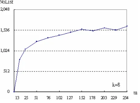
Complexity of Tag Initialization Algorithm.In the algorithm, there are N tags to be initialized; for each tag, the algorithm produces m pairs of (x, y); and for each y value, the algorithm searches the proximate value of y in the ylist using binary search. Here, we let the number of elements in the ylist be NoList. It is clearly that the NoList
of Tag Initialization Algorithm can be estimated as
m N
i NoListi
*
1 log( ).
Fig. 3. The average variation of the NoList
We let |Y"| be the maximum of NoList. The complexity of Tag Initialization Algorithm will be bounded by N*m*log(|Y"|) = N*m*log(2k") = N*m*k". Accordingly, it is sufficient that k" is set to 11 for k=8, also refer Figure 3.
Complexity of Tag Identification Algorithm. For each tag identification, the server searches y" in the ylist in order to map y" to y and then computes slope s to identify the tag. It takes log(|Y"|) = k" times in average, a const-time identification.
4. Performance Evaluations
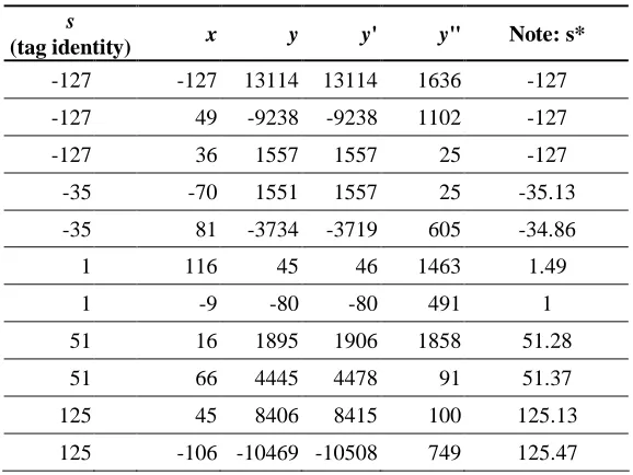
In this section, we use the results of experiments to evaluate the performance of the proposed scheme. The first experiment examines the compression effect of the proposed transformation algorithm on the y value. It adopts k=8 and chooses secret point (a, b) as (−23, −94). Then, it computes all (x, y, y', y") quartets, where (x, y) is the original point, y' is equal to y or the qualified adjacency of the y, and y" is the final result, a one-time random number. Figure 4 demonstrates part of raw data. For the rightmost column in Figure 4, it shows the slope, s*, which is computed by using (x,
y') and should be in the range of s plus or minus 0.5. To see the compression effect on
y, Figure 5 shows the distributions of (a): (x, y), (b): (x, y") and (c): (x, y") in smaller scale, respectively, when (a, b) = (−23, −94). Fig. 6 shows the same cases when (a, b) = (127, −127).
s
(tag identity) x y y' y" Note: s*
-127 -127 13114 13114 1636 -127 -127 49 -9238 -9238 1102 -127
-127 36 1557 1557 25 -127
-35 -70 1551 1557 25 -35.13
-35 81 -3734 -3719 605 -34.86
1 116 45 46 1463 1.49
1 -9 -80 -80 491 1
51 16 1895 1906 1858 51.28
51 66 4445 4478 91 51.37
125 45 8406 8415 100 125.13
125 -106 -10469 -10508 749 125.47
Fig. 4. Part of raw data for (a, b) = (-23, -94) in experiment 1
Fig. 5. The compression effect on y for (a, b) = (-23, -94) in experiment 1
The second experiment explores scalability and corresponding parameter selections. The goal of this experiment is to estimate the size of k" when k16. As we know, k" can be estimated by the order of Y". In the experiment, it randomly chooses (a, b), set
m as 250 (or 500), then executes Tag Initialization Algorithm five times, and finally computes the average number of elements in Y", denoted as |Y"|average. Table 2 shows
the results.
Table 2. The estimation of the size of k¡
k N m |Y"|average k"
16 65,534 250 470,365 (219) 19 500 498,700 (219) 19 20 1,048,576 250 6,180,011 (223) 23 500 10,077,000 (224) 24 22 4,194,310 250 47,100,995 (226) 26 500 108,205,904 (227) 27
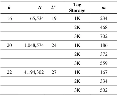
According to Table 2, we can estimate how many (x, y") pairs a tag can accommodate under different system scale and different tag storage. Table 3 shows the results.
Table 2. Parameter selection for different system scale
k N k" Tag
Storage m
16 65,534 19 1K 234
2K 468
3K 702
20 1,048,574 24 1K 186
2K 372
3K 559
22 4,194,302 27 1K 167
2K 334
3K 502
5. Security Analysis
We analyze the security of the proposed scheme in the following.
Privacy preservation. As shown in the proposed scheme, the proofs, (x, y") pairs, of a tag are different for each identification. These proofs play as one-time pads. Moreover, (x, y") can be treated as a random string since x is uniformly random while
y" is a random string generated by the server. Thus any two pairs (x1, y"1) and (x2, y"2)
the user location cannot be tracked when he bears something embedded with such a tag.
Against tag identity guessing. It is a very interesting property of our scheme that an adversary cannot guess the identity of a tag since he does not have any extra information about the real y from an eavesdropped y". Again, any two eavesdropped pairs (x1, y"1) and (x2, y"2) from a tag are just two random string and thus cannot
deduce the identity of the tag.
Against valid (x, y") guessing. An adversary might select an arbitrary sS and consider that it must be the identity of a tag in the system. However, without server's secrecy (a, b) he cannot determine the line for the tag. Even if he knows (a, b) and thus can computes (x, y), the adversary cannot map y to y" since the mapping table is preserved by the server. If the adversary uses random guessing, the successful probability of his randomly guessed (x, y") which can be accepted by the server is bounded by 2-(k+k").
Against (a, b) guessing. Any two lines representing two different tags can compute the interaction point, i.e. the point (a, b). However, without any clear y value, an adversary cannot determine any line. It is interesting that even when an adversary wants to exhaustively guess server's (a, b), he cannot succeed since none of clear (x, y) can be provided for examining his guessing. We refer to this security notion as
unconditionally secure.
6. Conclusion and future work
To our best knowledge, our scheme is the first attempt that uses a line on a plane to represent a RFID tag. It assures constant-time tag identification and thus possesses the scalability. Moreover, the random-looking response of a tag is changeable for each identification guards the user location privacy. This paper is just the beginning. Our future work are three aspects. The first is to find another better compression approach for y value to further downsize the space of storing y.
Secondly, the proposed scheme also requires a mechanism of updating (x, y") pairs in a tag. In our system described in Sec. 3, there will be no fresh (x, y") for a tag to respond server/reader's interrogations when m pairs of (x, y") are used. This will restrict the proposed scheme applied on many applications. A possible solution is that the server reallocates m fresh pairs to the tag via a secure channel.
addition, the server in Alomair's scheme must store all possible dynamic identities. The solution of RAP series is to launch brute search when the tag had suffered attacks. Although these solutions are not satisfactory, our future work may start from these works.
Reference
[1] S. A. Weis, S. Sarma, R. Rivest and D. Engels, Security and privacy aspects of low-cost radio frequency identification systems, Security in Pervasive Computing, March, 2003.
[2] M. Ohkubo, K. Suzuki and S. Kinoshita, Cryptographic approach to "privacy-friendly" tags, Proc. in RFID Privacy Workshop 2003, MIT, November 2003
[3] A. Juels, RFID security and privacy: a research survey, Journal of Selected Areas in Communication, 24(2) 381¡ 395, 2006.
[4] A. Juels and S. A. Weis, Defining strong privacy for RFID, ACM Transactions on Information and System Security, 13(1), Otc., 2009.
[5] D. Molnar and D. Wagner, Privacy and security in library RFID: issues, practices, and architectures, Proc. in 11th ACM Conf. Computer and Comm.Security (CCS
'04), Oct. 2004.
[6] J.S. Cho, S.S. Yeo and S.K. Kim, Securing against brute-force attack: a hash-based RFID mutual authentication protocol using a secret value, Computer Communications, 2010.
[7] G. Avoine, E. Dysli, and P. Oechslin, Reducing time complexity in RFID systems,
Selected Areas in Cryptography¡ SAC, 3897:291-306, 2005.
[8] L. Lu, J. Han, L. Hu, Y. Liu, and L. Ni., Dynamic key-updating: privacy- preserving authentication for RFID systems, International Conference on Pervasive Computing and Communications, 2007.
[9] G. Tsudik, YA-TRAP: Yet another trivial RFID authentication protocol, Proc. in 4th IEEE Int. Conf. Pervasive Computing and Comm. (PerCom'06), Mar. 2006. [10] T.V. Le, M. Burnmester, B.D. Medeiros, Universally composable and forward
secure RFID authentication and authenticated key exchange, Proc. in the Second ACM Symposium on Information, Computer and Communications Security, 242¡ 252, Mar. 2007,
[11] M. Burnmester, T.V. Le, B.D. Medeiros, G. Tsudik, Universally composable RFID identification and authentication protocols, ACM Transactions on Information and Systems Security, 12(4), 2009.
[12] D.N. Duc and K. Kim, Defending RFID authentication protocols against DoS attacks, Computer Communications, 2010.
privacy-preserving protocol with constant-Time identification, Proc. in the 40th Annual IEEE/IFIP International Conference on Dependable Systems and
Networks ¡ DSN '10, Chicago, Illinois, USA, June 2010, IEEE.
[14] B. Alomair, and R. Poovendran, Privacy versus scalability in radio frequency identification systems, Computer Communications, 2010.
[15] E. K. Ryu and T. Takagi, A hybrid approach for privacy-preserving RFID tags,
Computer Standards & Interfaces, 31, 812¡ 815, 2009.
[16] Y. K. Lee, L. Batina, and I. Verbauwhede, EC-RAC: Provably Secure RFID authentication protocol, Proc. in IEEE International Conference on RFID, 97¡ 104. IEEE, 2008.
[17] Y. K. Lee, L. Batina, and I. Verbauwhede, Untraceable RFID authentication protocols: revision of EC-RAC, Proc. in IEEE International Conference on RFID, 178¡ 185, IEEE, 2009.
[18] Y.K. Lee, L. Batina, D. Singelee and I. Verbauwhede, Low-Cost untraceable authentication protocols for RFID, Proc. in WiSec'10, New Jersey, USA, Mar., 2010.
[19] M. Burmester, B.D. Medeiros and R. Motta, Anonymous RFID authentication supporting constant-cost key-lookup against active adversaries, International Journal of Applied Cryptography, 1(2), 2008
[20] Y. Chen, J. S. Chou and H. M. Sun, A novel mutual authentication scheme based on quadratic residues for RFID systems, Computer Networks, 52, 2373¡ 2380, 2008.
[21] Y. K. Lee, K. Sakiyama, and I. Verbauwhede, Elliptic-Curve-Based Security Processor for RFID, IEEE Trans. on Computers, 57(11), Nov., 2008.
[22] G. Gaubatz, J. P. Kaps, E. Ozturk, and B. Sunar, State of the Art in Ultra-Low Power Public Key Cryptography for Wireless Sensor Networks, Proc. in the Third IEEE International Conference on Pervasive Computing and
Communications Workshops (PERCOMW'05), 2005.
[23] F. Gosse, F. X. Standaert, and J. J. Quisquater, FPGA Implementation of SQUASH, Proc. in the 29th Symposium on Information Theory in the Benelux, 2008.