The effect of shelter availability on foraging in Atlantic salmon (Salmo salar)

(1)

Western University Western University

Scholarship@Western

Electronic Thesis and Dissertation Repository

9-19-2018 9:30 AM

The effect of shelter availability on foraging in Atlantic salmon

(Salmo salar)

Christian A. Therrien

The University of Western Ontario Supervisor

Morbey, Yolanda E.

The University of Western Ontario Joint Supervisor Neff, Bryan D.

The University of Western Ontario Graduate Program in Biology

A thesis submitted in partial fulfillment of the requirements for the degree in Master of Science © Christian A. Therrien 2018

Follow this and additional works at: https://ir.lib.uwo.ca/etd

Part of the Aquaculture and Fisheries Commons, and the Behavior and Ethology Commons

Recommended Citation Recommended Citation

Therrien, Christian A., "The effect of shelter availability on foraging in Atlantic salmon (Salmo salar)" (2018). Electronic Thesis and Dissertation Repository. 5847.

https://ir.lib.uwo.ca/etd/5847

(2)

Abstract

Shelter is an environmental feature that provides protection from danger and its

use is an important anti-predator behavior for juvenile Atlantic salmon (Salmo salar).

However, how shelter availability influences the foraging of these fish in the wild is not

well documented. I predicted that juvenile Atlantic salmon would alter their foraging

behavior in a low shelter environment and that this effect would differ between

individuals from two populations that are targeted for reintroduction into Lake Ontario. I

measured the foraging activity of juvenile Atlantic salmon from the two populations

while they were held in pens in a Lake Ontario tributary that differed in their shelter

level. Particularly at midday compared to dawn and dusk, fish from both populations in

high shelter had a foraging rate and activity level approximately 2.6 times higher than

those in the low shelter. These differences in behavior had no noticeable association with

diet or growth rate during the experiment. The two populations tested did not differ in

their foraging behavior or growth based on the metrics tested. Overall, I found shelter can

influence foraging behaviour of Atlantic salmon and these effects are conserved between

populations.

Keywords

Predator-prey ecology, perceived predation risk, shelter use, foraging, growth, species

(3)

Acknowledgments

Thanks to everyone who helped me over the last two years as I took the next step

in my career in fish biology. A special thanks to my supervisors and mentors, Dr.

Yolanda Morbey and Dr. Bryan Neff for providing me with all the resources necessary,

whether it be advisory or financial, to be a successful researcher and graduate student.

Without them, I would not have been able to be successful. Thank you to my wonderful

advisors Simon Bonner and Liana Zanette for their helpful comments and advice on the

experimental design and for guiding me to produce a successful thesis. The entire

Morbey and Neff labs were an important source of support, assistance and guidance. I

would like to thank my lab mates Mat Stefan, Jessica Deakin, Niko Muñoz, Lucas

Silveira, Kim Mitchell, Babak Mehr, Adriano Cunha, Andrew Beauchamp, Olivia

Colling, Carlie Muir and Nicole Zathey. Special thanks to Mike Thorn for all his help and

guidance during my time at Western. Thanks to Shawn Garner for his help with

manuscript editing and experimental design. Many thanks for Nigel Davies for his help

collecting data in the field and for being a great research assistant.

Special thanks to Jake Ruegg and the OMNRF for providing the fish used in this

study and helping me with my experimental design. Thanks to Bill Sloan and the staff at

the Codrington Fish Culture Station for providing space to rear the juvenile salmon used

in this experiment and for their time spent caring for these fish. Thanks to the Toronto

Region Conservation Authority for allowing me to conduct my research at the

Greenwood Conservation Area. Thank you, Chris Guglielmo and his lab, for their advice

and guidance and for allowing me to use some of their equipment. Thanks to Scott

(4)

helping me set them up for my preliminary methods testing. Thanks to Zoe Lindo for

lending me some equipment for the invertebrate analysis and thank you James Pellerin

from the Maine DNR and Alex Levy from the DFO for providing me with electrofishing

surveys from the Crooked and LaHave Rivers, respectively.

(5)

List of Tables

Table 1. Number of foraging attempts model selection process using AIC.. ... 31

Table 2. The selected generalized linear mixed model with a zero-inflated Poisson

distribution showing the effects of treatment, diel period, and their interactions on the

number of foraging attempts of juvenile Atlantic salmon during the experiment.. ... 32

Table 3. Generalized linear mixed models with a zero-inflated Poisson distribution within

ΔAIC of 2 from the model with the lowest AIC showing the effects of treatment, diel

period, population and the population by treatment interactions on the number of foraging

attempts of juvenile Atlantic salmon during the experiment. ... 34

Table 4. Time active model selection process using AIC.. ... 35

Table 5. Generalized linear mixed models with a zero-inflated Poisson distribution within

ΔAIC of 2 from the model with the lowest AIC showing the effects of treatment, diel

period, population and the population by treatment interactions on the time active of

juvenile Atlantic salmon during the experiment. ... 36

Table 6. Results of generalized linear mixed models comparing the abundance of

(9)

List of Figures

Figure 1. Map of locations of the three riffle locations where the enclosures and drift net

were erected in East Duffins Creek at the Greenwood Conservation Area Ajax, ON….. 18

Figure 2. A) Schematic of Nitex net enclosure placement in a riffle section in East

Duffins Creek and B) image of enclosure erected in East Duffins Creek………. 19

Figure 3. Image of the weir used to recapture juvenile Atlantic salmon from the net pen

enclosures……….. 24

Figure 4. Histogram of the number of foraging attempts during each 10 minute

observation period overlaid with a Poisson distribution (black) with a λ = 1.15……….. 30

Figure 5. The number of foraging attempts per observation period and activity level of

Atlantic salmon from two populations during 6-day treatments in either high or low

shelter enclosures………... 38

Figure 6. Activity level of Atlantic salmon from either high or low shelter treatments at

each diel period during 6-day treatments in either high or low shelter enclosures for the

last 3 weeks of observations……….. 39

Figure 7. a) Activity level does not vary with food availability (r2 = 3.1 x 10-4). b)

Activity level does vary with water temperature (r2 = 0.08)………. 40

Figure 8. Histogram of the number of fish foraging during each 10 minute observation

period overlaid with a Poisson distribution (black) with a λ = 0.15……….. 42

Figure 9. The number of fish foraging in a pen during each observation period of Atlantic

salmon from the high and low shelter treatments at each diel period………43

Figure 10. Mean abundance of invertebrates of each order found in the stomachs of

Atlantic salmon of the LaHave River and Sebago Lake population after being held in net

(10)

Figure 11. Mass of food items in the stomach and gut contents of Atlantic salmon after

being held in net pens over 6 days………. 47

Figure 12. Specific growth rate of A) both the LaHave River and Sebago Lake

populations and B) of fish over the course of the experiment after 6 days in net pens of

either high or low shelter levels………. 48

Figure 13. Relationship between specific growth rate, stomach content mass and activity

level……… 49

Figure 14. Drifting A) Diptera (larvae, pupae, and adults), B) Ephemeroptera (larvae,

pupae), C) Trichoptera (larvae), and D) Total invertebrate drift catch per diel period and

day……….. 51

Figure 15. Environmental factors of East Duffins Creek over the course of the

(11)

List of Appendices

Appendix 1. List of aquatic predators present and their abundances in the tributaries of the two Atlantic salmon (Salmo salar) populations ... 92

Appendix 2.Experimental Protocol Approval Records.. ... 93

Appendix 3. Modified Latin squares design of treatment assignment per riffle sequence for each week of observations. ... 95

Appendix 4. Drift rates (individuals  m-3 hour-1; Median, 25th percentile, 75th percentile) of all invertebrate orders at each diel period captured with a drift net

(12)

Introduction

Anti-predator adaptations are complex, spatially and temporally variable, and are

sensitive to environmental cues and the life stage or condition of the organism. For

example, juvenile racers (Coluber constrictor) were more likely to show aggressive

behavior when encountered with a predator than were adult racers (Creer 2005). Daphnia

in high predator environments grow larger helmets and longer tail spines than those in

low predator environments (Krueger and Dodson 1981, Dodson 1989). Careful

perception of predation risk by prey is paramount and can have population level

consequences. Indeed, big horn sheep (Ovis canadensis) ewes differed in their boldness

depending on their local habitat and with yearly changes in predation pressure (Réale et

al. 2000). These differences in boldness translated to differences in reproductive success

as bold ewes started reproducing earlier and had a higher weaning success than did shy

ones (Réale et al. 2000). Understanding anti-predator behavior in natural systems and

during different times of the year is relevant for conservation and management, especially

of game species such as the aforementioned bighorn sheep and species at risk such as the

Atlantic salmon (Salmo salar).

Predation risk and avoidance

Throughout an organism’s life, predation risk can vary greatly. Predation risk may

vary at different life stages, seasonally, daily and even from one moment to the next.

Furthermore, predation risk also varies spatially as some environments have a greater

predation risk than others. As such, organisms will respond with antipredator defenses

differently according to these spatiotemporal variations in predation risks. These

(13)

differ in their body morphology depending on the level of predation in their environment

and use these changes in morphology as defenses against predation. For example,

three-spine stickleback (Gasterosteus aculeatus) will grow larger dorsal spines as a defense in

environments with high predation (Frommen et al. 2011). More often, when experiencing

high predation risk, organisms will modify their behavior and utilize behavioural

defenses to this risk of predation. Indeed, in environments with high predation risk or at

times of high predation risk, organisms may need to spend more time in shelter, change

their feeding behavior, select safer habitats, increase their vigilance and alter their escape

behavior (Lima and Dill 1990, Steiner 2007, Walters et al. 2017) compared to those with

low predation risk.

Predation is a major cause of mortality in the juvenile stages of fishes (Lima and Dill

1990). Several studies have shown size-selective mortality among fish, where small fish

are more likely to be predated upon than large fish (see review in: Sogard 1997).

Furthermore, in many species, such as largemouth bass (Micropterus salmoides) and

walleye (Sander vitreus), predation has been shown to be a major factor influencing

young of the year survival (Forney 1974, Post et al. 1998). For example, in 1983,

predation by walleye in Sparkling Lake, Wisconsin accounted for 80% of darter

(Etheostoma spp.) mortality (Lyons and Magnuson 1987).

In response to this predation, fishes have evolved many defenses against

predation. For example, fish may avoid areas where predation risk is high (Mikheev et al.

1994), reduce activity during periods when predation risk is high (Breau et al. 2007), and

use shelters to avoid detection by predators (Orpwood et al. 2006). Shelter is an

(14)

that provides protection from danger. Shelter use is an important anti-predator behaviour

and the use of shelters provides a refuge from predators and lowers prey vigilance

towards predators (Millidine et al. 2006, Larranaga and Steingrímsson 2015). However,

sheltering, like any antipredator behavior, can trade-off with foraging. A study on adult

two-spotted gobies (Gobiusculus flavescens) found that when gobies were introduced to

aquaria without predators, the addition of shelter had no effect on the time spent foraging

(Utne et al. 1993). However, in the presence of a predator, gobies spent the majority of

their time in shelter and less time foraging. The use of shelter can provide benefits

(reduced predation risk) but also has costs (reduced foraging; see also Tupper and

Boutilier 1997, Hösjesjö et al. 2004).

Traditionally, optimization models have been used to predict the behavior of prey

describing foraging while under predation risk. In these models, the central idea is a prey

animal can control its rate of energetic gain while controlling the probability that a

predator kills it. In these models, the control variable that characterizes an animal’s

behavior is u, where 0 ≤ u ≤ 1. Here, a large value of u would represent a high rate of

energetic gain and a high risk of predation and a small value of u would represent the

opposite (Houston et al. 1993). Several models (e.g. Milinski 1986, Sih 1987, Dill 1987)

have predicted that for an animal to have a high rate of energy gain it comes at the cost of

a high rate of predation. This “growth versus survival” trade-off can arise in various ways

including the choice of habitat (e.g. Schneider 1984, Lima 1987, Werner and Hall 1988),

level of vigilance (e.g. Elgar 1989, Lima 1990) and group size (e.g. Bertram 1978, Lima

1990, McNamara and Houston 1992). Gilliam (1982) theorized that organisms should

(15)

should attempt to minimize the ratio of mortality/growth. Using an optimization model,

this trade-off between growth and survival can be predicted given the rate of energetic

gain and risk of predation, in the notation of Houston et al. (1993) as,

M(u,x)/(a(x)u – b(x)),

where mortality due to predation is expressed as M and growth rate is expressed as a(x)u

– b(x) where a(x) is the rate of energy gain, b(x) is the rate of energy loss and x represents

a given state (Gilliam 1982). While studying the ontogenetic movement of sunfish

between habitats, Gilliam (1982) developed the M/ rule to predict when sunfish should

move between habitats that differ in their food availability and predation risk. The M/

rule states an animal would choose the life history stage or environment that maximizes

its growth () whilst minimizing its risk of predation (M; Gilliam 1982), and has been

used to predict the movement of several animals between habitats (Werner and Gilliam

1984, Werner 1986, Turner and Mittelbach 1990). However, these models do not take

into account time constraints such as the need to reach a size threshold by a given time or

physiological constraints such as gut size or satiation (Houston et al. 1993).

In fish, optimization models describing foraging under predation risk, such as

those by Fraser and Huntingford (1986), indicate that fish should adopt a risk-averse

foraging strategy to prioritize survival over growth. In this risk-averse strategy,

organisms are expected to avoid the hazard and minimize the consumption of food,

especially at times of high-predation and in environments with a high risk of predation.

Empirically, this has been shown in a number of taxa and species including ants (Lasius

pallistarsis; Nonacs and Dill 1990), stickleback (Gasterosteus aculeatus; Fraser and

(16)

others (see review in: Preisser et al. 2005). However, other models have shown that the

risk-averse strategy is not always optimal. For example, models by Houston et al. (1993)

suggest if there is no refuge nearby, then it is optimal to maintain foraging behavior

constant despite predation risk.

When time constraints are introduced into these models, the predicted behavior of

organisms differs greatly than what is predicted by traditional models. In this context,

time constraints are limitations that an animal has to grow to a certain size before it can

complete some aspect of its life history, such as reproduce or migrate, and imply that

foraging behavior can change over time (Gilliam 1982, Ludwig and Rowe 1990, Rowe

and Ludwig 1991).These time constraints such as diapause in insects (Ludwig and Rowe

1990) or metamorphosis in amphibians (Werner 1986) present an interesting case where

organisms must reach a size threshold by a certain time or there may be fitness

consequences. For example, the drying of ephemeral pools represents a severe time

constraint in which an amphibian will die if it has not metamorphosed by the time the

pool has dried (Werner 1986). Models where a time constraint is introduced such as

Ludwig and Rowe (1990) suggest organisms take a more risk-reckless approach to

foraging where organisms partake in riskier foraging behavior, even when predation risk

is high, in order to reach the size threshold.

When the environment offers little to no protection to prey, prey may have little to

no choice than to forage despite a risk of predation. In these environments that offer low

protection from predators, prey may find protection in their size rather than from the

environment. Size refuge theory suggest the accelerated development of some organisms

(17)

1997). Indeed, in caterpillars such as the tobacco hornworm (Manduca sexta), the rapid

development of early instars to later instars may lower predation risk (Thaler et al. 2012,

2013). Later instars have larger head capsules with larger mandibles and have thicker

cuticles than earlier instars and these morphological traits better allow them to defend

themselves (Thaler et al. 2012, 2013). While this has been described in insects,this

pattern can also occur in fish. In fish populations, within-cohort size-selective mortality is

often observed can can occur as early as the egg stage (Rijnsdorp and Jaworski 1990),

although much of the research is focused on the larval stage of fish, where as juvenile

size increases, capture success from predator decreases (e.g. Fuiman 1989, Litvak and

Legett 1992, Juanes and Conover 1995). In stream fishes, the majority of their predators

are gape-limited meaning once a prey fish has grown larger than the gape of the predator,

it cannot be predated upon. In fish whose predators are gape-limited, increased individual

growth can result in a shorter period of susceptibility to these predators (Persson et al.

1996, Sogard 1997).

Daily activity budgets

Increases in perceived predation risk may also result in unpredictable and variable

interruptions in foraging. Because of this, organisms can also change their foraging

behaviour to avoid foraging at times of high predation and increase their activity at times

of perceived safety (Lima 1986, Houston and McNamara 1993, McNamara et al. 1994,

2005, Sih and McCarthy 2002, MacLeod et al. 2007, Creel et al. 2008, Walters et al.

2017). This “interrupted foraging” response has been observed in a number of taxa

including birds (Lima 1986, Houston and McNamara 1993, McNamara et al. 1994, 2005,

(18)

crepuscular (dawn and dusk) in response to high predation risk from diurnal predators

(Gries et al. 1997, Metcalfe et al. 1998, 1999). Attacks from diurnal predatory lizardfish

(Synodus intermedus) during the dusk migration of juvenile grunts (Haemulidae) to

foraging grounds caused grunts to delay their migration until past sunset in order to avoid

being attacked (Helfman 1986). Within a species, shelter availability can influence the

diel timing of foraging in salmonids. For example, juvenile Arctic char (Salvelinus

alpinus) forage primarily during twilight hours in high shelter environments to minimize

encounter rates with diurnal avian predators and forage during daylight hours in low

shelter environments (Larranaga and Steingrímsson 2015). Juvenile Atlantic salmon in

artificial streams display similar behaviour with increased nocturnal activity in the

presence of cover compared to the absence of cover (Orpwood et al. 2010). In low shelter

environments, studies have shown fish prioritize growth over survival by foraging during

times of high food availability while increasing their vigilance (Orpwood et al. 2010,

Larranaga and Steingrímsson 2015). The prioritization of growth over survival could be

due to the fact that the majority of fish predators are gape-limited and increased

individual growth can result in a shorter period of susceptibility to these predators

(Persson et al. 1996, Sogard 1997) but this theory remains controversial as it suggests

prey animals should put themselves in situations with higher predation risk in order for

future protection from predators (Lima and Dill 1990).

Population differences in foraging behaviour

The intensity, or frequency and duration, of anti-predator behaviours is often

correlated with levels of predation that are experienced by prey populations under natural

conditions (Bell 2005). As such, the response to predators may differ among populations

(19)

example, three-spined stickleback (G. aculeatus) from the Navarro River, an environment

with high predation rate, remained motionless longer and foraged less following a visual

cue of a predator, than those from Putah Creek, an environment with low predation rate

(Bell 2005). Population differences in anti-predator behaviour have also been noted in

shelter use. Fathead minnows (Pimephales promelas) from a population allopatric with

predatory northern pike (Esox lucius) did not change shelter use when exposed to a visual

stimulus of pike (Mathis et al. 1993). However, when shown a visual stimulus of pike,

minnows from a population sympatric with pike increased shelter use (Mathis et al.

1993). Thus, populations of prey species may differ in their intensity of antipredator

behaviours in accordance to the perceived predation risk in the environment.

Effect of predation on diet and physiological processes

While under risk of predation, prey species may choose to trade-off some aspect

of their diet. One aspect they may trade-off is the amount of food consumed.

Predator-induced reduction in food consumption has been observed in a number of studies and

“scared prey typically eat less” (Zanette et al. 2014). This predator-induced reduction in

food consumption has been observed in a number of taxa such as in caterpillars (Thaler et

al. 2012, 2013), Trinidadian guppies (Dalton and Flecker 2014) and Atlantic salmon

(Metcalfe et al. 1987).

Additionally, the risk of predation is known to change the diet of prey species.

While under risk of predation, studies have shown prey may choose to feed on less

palatable food in order to avoid predation (Hawlena and Pérez-Mellado 2009,

Christianson and Creel 2010). However, these diet changes could be influenced by the

(20)

selectivity of prey species in one of two ways (Hawlena and Schmitz 2010a). First, prey

can alter their selectivity from nitrogen-rich to carbohydrate-rich foods. This allows for a

greater store of carbohydrates to be used as energy in order to be able to escape predators

and compensate for the increase metabolic rate in the presence of predators (Hawlena and

Schmitz 2010b). Second, prey demands can change from carbohydrate rich to nitrogen

rich macronutrients in a shift from maintenance to growth (Rosenblatt and Schmitz

2016). In aquatic environments, it is proposed the increased nitrogen consumption is

needed to increase the development rate of locomotor traits to allow prey to escape their

predators (Costello and Michel 2013, Dalton and Flecker 2014, Guariento et al. 2015,

Rosenblatt and Schmitz 2016). This has also been observed in red-legged

grasshoppers (Melanoplus femururbrum) under predation risk from a sit and wait

predator to change their locomotor traits to enhance their escape performance (Rosenblatt

and Schmitz 2016).

Paired with predation-induced changes in behavior and foraging are changes to

physiological processes. Predation is known to increase the maintenance metabolism of

prey as a result of prey increasing their vigilance and the metabolic stress imposed by the

risk of predation (see review by: Clinchy et al. 2012). This metabolic stress can greatly

reduce the growth rate of prey (Slos and Stoks 2008, Slos et al. 2009, Hawlena and

Schmitz 2010b, Culler et al. 2014, Schmitz et al. 2016). To combat these depressed

growth rates induced by predation risk, studies have shown prey can alter their food

assimilation and nutrient retention to maintain growth rates (Thaler et al. 2012, 2013,

Dalton and Flecker 2014). For example, Thaler et al. (2013) found that although tobacco

(21)

predator, they grew at the same rate as unthreatened conspecific. It was found that the

caterpillars increased digestive and assimilation efficiencies under risk of predation

(Thaler et al. 2012, 2013). Furthermore, a study on Trinidadian guppies (Poecilia

reticulata) found that although guppies reduce nutrient intake while under risk of

predation, their nitrogen retention effiency increased (Dalton and Flecker 2014). The

authors suggested the increased nitrogen retention was to fuel the protein-consuming

physiology induced by predation risk (Hawlena and Schmitz 2010b, Dalton and Flecker

2014). However, these counter mechanisms to predation induced stress have their costs.

Thaler et al. (2013) found that these increases in physiology ceased to occur during

longer term assays and caterpillars that used these mechanisms had changes to

development and body composition later in life (Thaler et al. 2012). Alternatively,

metabolic stress may be so great that assimilation effiencies decrease further exacerbating

decreases in growth rate (Hawlena and Schmitz 2010b, Culler et al. 2014, Schmitz et al.

2016).

Study species

Atlantic salmon are visual predators that are primarily active during the day

during the summer months and feed on drifting invertebrates. While juveniles, Atlantic

salmon mostly feed on drifting invertebrates and are diet generalists, feeding on what is

available in the drift (Allen 1941, Keeley and Grant 1997). To feed, Atlantic salmon will

leave a shelter, such as behind a submerged boulder or woody debris, and hold

themselves in areas of higher current waiting for drifting invertebrates to pass

(Wańkowski and Thorpe 1979, Huntingford et al. 1988). This holding position is defined

(22)

feeding efficiency, or the success rate of capturing prey items for a given foraging strike,

while station keeping during the day (Fraser and Metcalfe 1997).

Although foraging efficiency is high during the day, so is the risk of predation by

diurnal predators (Gotceitas and Godin 1991, Fraser and Metcalfe 1997). In the stream

environment, the major predators of juvenile Atlantic salmon are diurnal avian predators

such as mergansers (Mergus spp.) and kingfishers (Megaceryle spp.) and larger diurnal

piscivorous fish such as brook trout (Salvelinus fontinalis) (White 1937, 1938, Gotceitas

and Godin 1993). At times of low light intensity, both predation risk and foraging

efficiency are expected to be lower than during the day.

During the first year of their juvenile life, Atlantic salmon undergo threshold

dependent survival. In their first winter, the combination of low water temperatures

causing slow movement speed making capturing food items difficult and low food

availability in stream environments result in juvenile Atlantic salmon undergoing a

period of anorexia (Metcalfe et al. 1986, Metcalfe and Thorpe 1992). To survive the first

winter, young of the year salmon must reach a critical energy threshold of 4400–4800 J 

g-1 (Finstad et al. 2004). Indeed, depletion of stored energy has been suggested to be a

major cause of overwinter mortality in juvenile temperature fishes (Gardiner and Geddes

1980; Post and Evans 1989, Miranda and Hubbart 1994). Furthermore, the survival rate

of juvenile salmon is correlated with their body size (Feltham 1990, Mangel 1996), as is

reproductive success (Garant et al. 2001, 2002). There is thus a fitness imperative to be

large as a juvenile salmon (Mangel 1996, Garant et al. 2001, 2002).

Environmental influence on foraging and shelter use

Past research has examined the effect of water temperature, life history stage, time of

(23)

salmon in a laboratory setting (Metcalfe et al. 1986, 1998, 1999, Metcalfe and Thorpe

1992, Orpwood et al. 2006, Millidine et al. 2006). Being ectotherms, Atlantic salmon are

sensitive to temperature and adjust their growth and foraging accordingly. During the

summer, high water temperatures cause Atlantic salmon to forage primarily during the

day when their metabolic rates are at their highest (Fraser and Metcalfe 1997). Atlantic

salmon have high visual acuity during the day and have higher capture efficiency than at

night (Fraser and Metcalfe 1997). Diurnal foraging is more profitable in terms of food

gained per unit time, but is also riskier than foraging at night (Clark and Levy 1988). As

water temperature decreases as summer progress to autumn, nocturnal foraging has been

found to increase as the daily energy requirements of juvenile Atlantic salmon also

decreases (Fraser et al. 1993, Fraser and Metcalfe 1997). Because their energetic

requirements are lower in colder water temperatures, Atlantic salmon can afford to forage

at night when the risk of predation is lower. Indeed at low water temperatures, Atlantic

salmon have been found to preferentially seek shelter during the day (Fraser et al. 1993).

Food availability is also known to influence the daily activity budgets of Atlantic

salmon. During times of high food availability, several laboratory-based studies have

shown Atlantic salmon to preferentially shelter during the day and opt to forage at night

(Metcalfe et al. 1999, Orpwood et al. 2006). It is thought the high food availability offsets

their reduced foraging efficiency at night. The opposite can also be said during times of

low food availability, as Atlantic salmon will preferentially forage during the day to

maximize successful encounters with drifting prey (Metcalfe et al. 1999, Orpwood et al.

(24)

day and studies have shown drifting invertebrate drift exhibit diel periodicity with highest

invertebrate drift at night (Elliott 1969, Douglas et al. 1994).

Prior work on the Atlantic salmon foraging and predation risk have focused on the

influence of predation risk on the social status of salmon and how it relates to time to

resumption of foraging after a disturbance, but did not focus on the timing of foraging

(Gotceitas and Godin 1991). Furthermore, a study by Orpwood et al. (2010) examined the

effect of shelter availability while foraging and found that fish in high shelter enclosures

reduced their day time foraging and opted to increase foraging at night. However, this

study was performed in an artificial stream without predation cues and at a constant

temperature. As a result, a change in timing of foraging as a response to in-stream shelter

availability has not been studied within a natural field environment where juvenile

Atlantic salmon are exposed to the ambient risk of predation

Lake Ontario’s Atlantic salmon

Atlantic salmon are a species of interest in Ontario and are the target of

reintroduction efforts. Originally extirpated in the late 1800s (Crawford 2001), past and

present stocking attempts have yet to reestablish a self-sustaining population (Stewart and

Johnson 2014). In response to these past stocking attempts, the Ontario Ministry of

Natural Resources and Forestry (OMNRF) and the Ontario Federation of Anglers and

Hunters (OFAH) in 2006 launched the Lake Ontario Atlantic Salmon Restoration

Program (LOASRP), a 20-year restoration program combining habitat restoration,

research, education and large scale Atlantic salmon stocking efforts with the goal of

restoring self-sustaining Atlantic salmon populations in the Great Lakes. Currently, the

OMNRF stocks juvenile fish from two populations of Atlantic salmon into Lake

(25)

salmon from these populations have been isolated for thousands of years and there is no

possibility of gene flow among the populations (King et al. 2001). These two populations

of Atlantic salmon have different captive breeding histories in Ontario. The LaHave

River population of Atlantic salmon has been propagated in OMNRF hatcheries since

1989 and has spent 6 generations in the hatchery setting (Ontario Ministry of Natural

Resources 2011). On other hand, the Sebago Lake population of has been propagated in

OMNRF hatcheries since 2007 in OMNRF hatcheries and has spent 3 generations in the

hatchery setting (Houde 2015). Historically, the two populations likely experience

different predation regimes as juveniles their native tributaries (Appendix 1) that may

have led to evolved differences in anti-predator behavior. For example, the LaHave River

population of Atlantic salmon encounter more diurnal predators than does the Sebago

Lake population and this difference in predation regime could lead to differences in the

intensity of antipredator behaviours. Indeed, Atlantic salmon progeny from a cross

between parents from the LaHave River population and wild Mersey River populations

spent more time motionless, more time in shelter and performed fewer foraging strikes

than did fish from the Sebago Lake population (Lau 2016). This result suggests that fish

from the LaHave population might be more risk-averse than fish from the Sebago

population.

Research Objectives and Hypotheses

The two objectives of this study were to test if low shelter availability decreases

the rate and changes the timing of diel foraging in Atlantic salmon and to assess if these

effects differ between the two Atlantic salmon populations used for reintroduction into

(26)

foraging. Thus, I predicted that with a lower shelter availability, fish would forage less

and prioritize predation avoidance. Furthermore, I predicted that in a low shelter

environment, fish will forage more heavily at night in order to minimize the risk of

predation from diel predators. In a high shelter environment, fish should forage more

during midday, taking advantage of a time when foraging efficiency is highest given their

visual hunting strategy. Furthermore, I predicted that if fish foraged less with a decrease

in shelter availability, then fish in environments with low shelter availability should have

lower growth rates and lower gut content masses than those in environments with high

shelter availability. Additionally, given that predation risk can influence diet, I predicted

that fish in environments with low shelter availability would have a different diet

compared to those in an environment with high shelter availability. Assuming evolved

differences between populations, I predicted that the LaHave fish, which have more

diurnal predators in their native environment than fish from the Sebago population, will

(27)

Methods

Study populations

The experimental protocol used in this thesis was developed in accordance with

the guidelines of the Canadian council on Animal Care as well as the Ontario Ministry of

Natural Resources and Forestry and University of Western Ontario Animal Care

Committees (Appendix 2). Juvenile salmon were bred from sexually mature age 3 males

and age 4 females reared at the Ontario Ministry of Natural Resources and Forestry

Normandale Research Facility (Vittoria, ON) on 2 November and 17 November 2017 for

the Sebago Lake and LaHave River populations, respectively. Approximately 18,000

eggs were collected from 30 females per population and were fertilized with the milt

from a unique male in a 1:1 breeding design. After fertilization, the eggs were transferred

to an 8-tray vertical incubator (Marisource, Fife, WA). Fish were exposed to

photoperiods that best matched the local conditions and were exposed to the same water

temperatures experienced by a nearby stream (Normandale Creek). Eggs were incubated

in these conditions until yolk sac absorption (127 days, ~1000 degree days). After yolk

sac absorption, they were transferred to the Codrington Fish Culture Station (Codrington,

ON) into white 73 L polypropylene tanks. Each tank was divided in two with a grey

Plexiglas divider with a piece of grey astroturf held on the bottom of the tank with a piece

of stainless steel in each corner of the piece of astroturf. Fish were exposed to a natural

light cycle and water temperatures from the nearby stream (Marsh Creek). Here, the fish

were transitioned to exogenous feeding. Fish were fed with approximately 100 mg of fish

meal pellets per g of fish biomass hourly from 9:00 to 17:00 daily. Fish were reared at

(28)

Upon reaching the parr stage, fish were tagged and allowed to recover before they

were stocked into net pen enclosures. Seventy-two juvenile salmon from each population

were haphazardly selected, size matched in pairs to minimize any size effects that could

influence foraging behavior, anesthetized in a bath of tricaine methanesulfonate

(MS-222; 15 mg/L) and sodium bicarbonate (15 mg/L) then tagged with a subcutaneous

injection of fluorescent visual implant elastomer tags (VIE; Northwest Marine

Technologies, Shaw Island, WA) on the dorsal surface of the back to allow for individual

identification. After tagging, fish were given two weeks time to recover from the tagging

procedure before they were stocked into net pens. Prior to stocking, the mass (± 0.1 g)

and fork length (± 0.1 mm) of each juvenile salmon was measured.

Field site and net pen design

Experiments were conducted in East Duffins Creek, Ontario, Canada (Figure 1)

between 1 August and 11 September 2017. Enclosures (described below) were erected in

three riffle sequences, the preferred habitat for juvenile Atlantic salmon (McCrimmon

1954). Six synthetic nylon net enclosures (4 mm stretched mesh size) measuring 1.5 m x

1 m x 0.75 m (length x width x height) were secured lengthwise in the creek. The

enclosures were assembled as panels with 2.54 x 5.08 cm white pine strapping as the

frame with the synthetic nylon mesh stapled to the frame. The panels were fastened

together using 20 cm cable ties and secured to the streambed using 2.44 m steel alloy

t-bars. Wires were stretched across the top of the enclosure to deter avian predators. A pair

(29)

Figure 1. Map of locations of the three riffle locations where the enclosures and drift net were erected in East Duffins Creek at the Greenwood Conservation Area Ajax, ON.

Satellite images were obtained from Google maps

(http://maps.googleapis.com/maps/api/staticmap?center=46.34,-80.6755) and the map

was created using package ggmap (Kahle 2018).

200m

Longitude

L

a

titu

d

(30)

Figure 2. A) Schematic of Nitex net enclosure placement in a riffle section in East Duffins Creek and B) image of enclosure erected in East Duffins Creek

(31)

Experimental design

Each enclosure received a shelter treatment (high or low) and fish from either the

LaHave or Sebago Lake population based on a modified Latin squares design (see

Appendix 2). The low shelter treatment was composed of a thin layer of natural substrate

(sand, silt and gravel) with one added boulder of approximately 20 cm in diameter placed

on top of the substrate (Dolinsek et al. 2007, Bilhete and Grant 2016). The high shelter

treatment was composed of the same substrate as the low shelter treatment but included

five boulders of approximately 20 cm in diameter. The natural substrate was a mixture of

pebbles (<5 cm in diameter), gravel (0.2 cm–1.0 cm), silt, and sand. The natural substrate

was sieved to exclude particles >5 cm to ensure all treatments had substrate of the same

size. The added boulders, which were size and shape matched by eye, were collected

from other parts of the stream within the vicinity of each riffle and were scrubbed with a

brush with stiff bristles to remove any potential food. Each enclosure was marked in 10

cm increments, on the outside edge of the mesh, both parallel and perpendicular to the

stream axis, in order to create a Cartesian coordinate system that was used to obtain

coordinates for fish locations to keep track of foraging stations and sheltering locations

for each individual in a pen.

Each enclosure was stocked with four Atlantic salmon juveniles, a density used in

previous net pen studies (Larranaga and Steingrímsson 2015, Bilhete and Grant 2016).

Fish were given one day to acclimate to the enclosures before undergoing behavioural

observations. One day appears to be enough time for the Atlantic salmon to acclimate and

matches previous behavioural net pen studies (Larranaga and Steingrímsson 2015,

(32)

potentially increase food availability, and placed back in the pens. This process was

repeated an additional five times so that each treatment and each population was

measured in each enclosure. In the fourth sampling week of the study, from 23 August

2017 to 28 August 2017, a high flow event caused a large log to crash into one of the net

pen enclosure in riffle 2 that contained fish from the LaHave River population in the high

shelter treatment. Upon impact, the log broke the cable ties on the upstream panel and

opened a gap in the enclosure. No fish were sighted during the week of observations and

no fish were recaptured at the end of the week. As such, this experimental unit (week 4,

pen 2, riffle 2) was excluded from all analyses. The number of experimental units was 35.

Behavioural observations

During 6-day trials, 10-minute observations were conducted on fish four times

daily within 2 h blocks of time: dawn (from sunrise to two hours after sunrise), mid-day

(between 11:00 and 3:00), dusk (two hours prior to sundown to sundown), and night

(between 21:00 and 23:00) for a total of 24 observations per enclosure per week. Sunrise

and sunset times were obtained daily from Environment Canada for Pickering, ON

(https://weather.gc.ca/city/pages/on-54_metric_e.html). One observer stood motionless

downstream from the enclosures and began observations after five minutes by searching

for fish. Once a fish was detected, it was observed for 10 minutes and the observer

recorded the number of foraging attempts made and the time a fish spent active. Once all

detectable fish in each pen were observed, the number of fish foraging per pen during

each sampling period was also determined. The number of foraging attempts was

measured as the number of foraging attempts during the 10-minute observation period. A

foraging attempt is defined as a movement of more than one body length to capture a

(33)

swimming movement and afterwards, juvenile salmon return to their foraging station. A

fish was considered active if it was not motionless in the substrate or hiding under a

shelter during the 10 minutes. The time fish were active was measured as time each fish

was active was recorded during the observation period measured in seconds. Because fish

were not always active, observation times varied between 15 minutes to 45 minutes for

each pen. If after 15 minutes of observation no fish were detected, it was assumed that all

fish in the pen were sheltering. During the night sampling period, observations were

carried out with infrared cameras to eliminate the use of flashlights, since light of shorter

wavelengths is known to influence fish behavior (Marchesan et al. 2005). Because of the

difficulty of observing fish using infrared cameras, I was unable to measure the foraging

rate of fish during the night diel period but was able to measure their time active and the

number of fish foraging. Unusually high levels of precipitation throughout the first three

weeks of the experiment resulted in higher than average discharge and high turbidity

making night time observations difficult. As a result, night time observations were only

available for the final three weeks of the experiment. After six days of observations, the

salmon were euthanized in a bath containing MS-222 and weighed (± 0.1 g). Once

euthanized, the digestive tract of each fish was collected and stored in 95% ethanol for

further analysis.

Stomach content analyses

To assess foraging success and short-term growth, attempts were made to recover

all fish at the end of each 6–day trials. Since Atlantic salmon parr are known to seek

refuge in the interstitial space between substrate as an anti-predator behavior

(34)

at the end of each week. The weir measured 1.1 m x 1 m x 1 m (length x width x height)

with a 1 m opening at the beginning of the weir ending with a 15 cm opening 80 cm from

the front of the weir (Figure 3). The frame of the weir was constructed from 2.54 x 5.08

cm white pine strapping with 4 mm opening sized synthetic nylon mesh. To remove fish

from each enclosure, the downstream panel of the enclosure was removed by cutting the

cable tie fasteners and the weir was fastened to the t-bars where the panel had been. Once

secured, the base substrate was disturbed with a rake and fish were corralled into the

weir. Using this method, the recapture efficiency was 66%. As a result, only 90 fish were

recaptured and could be used for stomach content analyses and could have their growth

rates calculated.

To remove the stomach contents from the preserved stomachs, a cut was made

along the stomach with a scalpel. The stomach contents were then flushed from the

stomach into a 39 mL Bogorov tray using an 80% ethanol solution. After flushing, items

still stuck to the stomach lining were removed using a pointed probe. All stomach

contents were then examined under a stereozoom microscope to determine foraging

success (invertebrate abundance) and diet (invertebrate richness) of each individual (Grey

2001). Invertebrates found in the stomach were identified to order using a key found in

Peckarsky et al. (1990). After examination, stomach contents were filtered from the

ethanol solution using a 15 mL milipore vacuum filter (Fisher Scientific, Ottawa, ON)

with a pre-weighed 2.4 cm Whatman glass microfiber filter paper (Fisher Scientific,

Ottawa, ON). Once the ethanol was removed, the filter paper with the stomach contents

(35)

(36)

weighed (± 0.1 mg) then placed in a 60 °C oven (VWR International, Mississauga, ON)

for 24 hours. The dry stomach contents and their filter paper were then weighed (± 0.1

mg). The mass of the intestine contents was also measured. Intestine contents from each

fish were flushed from the intestines onto a weigh boat using deionized water. After

flushing, items still stuck to the intestinal lining were removed using a pointed probe. The

weigh boats with the intestine contents were weighed (± 0.1 mg) then placed in a 60 °C

oven (VWR International, Mississauga, ON) for 24 hours. The stomach content and

intestine content dry masses were added to determine total gut dry mass.

Physical parameters

Physical parameters, including water depth (± 1 cm) and water temperature (± 0.1

°C) for each site were measured every 15-minutes with HOBO U20L loggers (Onset Inc.,

Bourne) and HOBO Pendant Temperature/Light 8k loggers (Onset Inc., Bourne). Current

velocity (m/s) was measured at the start of each observation period with a Flowtracker

(Sontek, San Diego). Physical parameters were measured because temperature and

current velocity are known to influence the foraging behavior of Atlantic salmon

(Wańkowski and Thorpe 1979, Metcalfe et al. 1998).

To determine the drifting invertebrate availability during each sampling period, a

drift net (30 cm x 40 cm mouth x 80 cm long, 250 μm mesh) with a collection bottle (5

cm x 7.5 cm) was installed upstream from the first riffle (Figure 1). The drift net was

deployed four times daily at the same time behavioural observations took place. Bottle

contents were then collected and preserved in 2000 mL of 95% ethanol. From each 200

mL sample, two 39 mL subsamples were randomly selected and placed in a 39 mL

Bolgorov tray (Wildco, Yulee, Fl). Invertebrates present in each subsample were counted

(37)

Peckarsky et al. (1990). Night time drifting invertebrate data was not available for weeks

1–3 of the experiment since drift nets were deployed only when behavioural observations

were performed.

Data Analyses

All analyses were conducted in R 3.5.0 (R Core team 2018). For each diel period,

behavioural metrics were averaged among individuals in a pen and over the 6-day trial

prior to further analysis to avoid pseudoreplication. The distribution of the number of

foraging attempts was first determined using the function fitdistr with the package MASS

(Ripley 2018). Foraging rate data were then analyzed using fully factored Poisson

generalized linear mixed models in the package glmmADMB (Coxe et al. 2009, Skaug et

al. 2010). The time fish were active was first normalized using a ln(x + 0.1)

transformation, then analyzed using generalized linear mixed models with Gaussian

distribution in with the function lmer in the package lme4 (Bates et al. 2018). To compare

the time fish were active between treatments at night, the transformed data were

compared using an unpaired two sample Wilcoxon test. Akaike Information Criterion

(AIC) was used for model selection among all possible models. Random effects were

initially included in models but were removed if they did not explain any of the variance

(i.e. var = 0, SD = 0).

The number of fish foraging was analyzed using a Poisson generalized linear

mixed model in the package glmm (Knudson 2018) with 105 Monte Carlo likelihood

approximations. A Poisson regression model was analyzed to test the effects of treatment,

diel period (i.e. dawn, midday, etc…), population, and included random intercepts for

(38)

the experimental unit). Subject was included to deal with the repeated nature of the

activity data across diel periods.

Stomach invertebrate abundance for three most common invertebrate orders were

analyzed using Poisson generalized linear mixed models in either the package

glmmADMB (Skaug et al. 2010) if the data fit a zero-inflated Poisson distribution or in

the package glmm (Knudson 2018) with 105_{Monte Carlo likelihood approximations if}

the data fit a Poisson distribution (Coxe et al. 2009). Poisson regression models were

analyzed for each stomach invertebrate order to test the effects of treatment, population,

the population by treatment interaction and included random intercepts for week number

(1–6), riffle number (1–3) and pen (1–6). The dry and wet mass from the total stomach

contents and the total gut content dry mass were first normalized using a ln(x + 1)

transformation, then analyzed using a generalized linear mixed model with Gaussian

distribution in with the function lmer in the package lme4 (Bates et al. 2018). Generalized

linear mixed models fit with a Gaussian distribution were developed for all three metrics

to test the effects of treatment, population, the treatment by population interaction,

included fish length as a covariate as well as sampling week, riffle and subject as random

effects.

Fish mass and length was compared using a generalized linear model with a

Gaussian distribution to assess if there were size differences between fish in each

treatment, between populations, if there was a treatment by population interaction and

across weeks. Specific growth rate for each individual fish was calculated using the

methods by Ricker (1975) according to the following equation:

(39)

where M is the mass of the fish and t is the duration of the experiment in days. SGR was

first ln(x+1) transformed to normalize the data then compared between treatments and

populations using generalized linear mixed models with a Gaussian distribution. A

Gaussian model was developed to test the effects of treatment, population, the population

by treatment interaction and included fish length as a covariate as well as week, riffle and

subject as random effects. Linear regression analyses were used to determine the

relationship between both stomach content wet and dry mass to specific growth rate.

Linear regression analysis was also used to determine the relationship between activity

level and specific growth rate.

Food availability was determined by determining the drift rate of the invertebrates

most consumed by juvenile Atlantic salmon. Drift rate was estimated using the equation:

D = (I/AV)/t

where D is the invertebrate drift rate, I is the number of invertebrates in the drift net

sample, A is the sampling area of the drift net, V is the water velocity while the drift net

was deployed, and t is the amount of time the drift net was deployed in hours (O’Hop and

Wallace 1983). The invertebrate drift rate is measured as number of individuals · m-3·

hour-1 and drift rates were calculated for all orders. Summary means were produced for

each order during each time of day (dawn, dusk, midday, night) over the course of the

experiment. Linear regression analysis was used to determine the relationship between

activity level and food availability.

Summary means for water temperature and discharge data were produced for each

time of day over the course of the experiment. Linear regression analysis was used to

(40)

Results

Population differences in body size

At the start of the experiment, Sebago Lake fish were longer (mean ± SD; 7.6 ±

0.9 cm) than LaHave River fish (6.6 ± 0.7 cm, t= 8.2, df = 139, p < 0.01). Fish from the

Sebago Lake population were also heavier (3.9 ± 1.4 g) than those from the LaHave

River population (2.3 ± 0.8 g, t = 9.4, df = 139, p < 0.01). There was no difference in the

length (t = 0.76, df = 139, p = 0.45) and mass (t = 0.68, df = 139, p = 0.49) of fish used in

high versus low shelter treatments. Fish length (t = 6.42, df = 139, p < 0.01) and mass (t =

5.64, df = 139, p < 0.01) increased with week number. At the end of the experiment, fish

from the Sebago Lake population continued to be heavier (4.1 ± 1.5 g) than those from

the LaHave River population (2.5 ± 0.8 g, t = -6.3, df = 71, p < 0.01).

Foraging rate, time active and number of fish foraging

The number of foraging attempts best fit a zero-inflated Poisson distribution

compared to a Gaussian or Poisson distribution (Figure 4). The top model based on

having the lowest AIC included treatment, diel period and their interaction (Table 1), but

not population. The average number of foraging attempts was approximately 2.6 times

lower in the low shelter treatment (0.7  1.9 strikes, N = 18) than in the high shelter

population (1.8  2.8 strikes, N = 17, p = 0.01, Figure 5a, Table 2). Fish had a higher

number of foraging strikes during midday (1.9  3.2 strikes, N = 35) than at dusk (1.1 

2.7 strikes, N = 35) and dawn (0.5  1.8 strikes, N = 35, p < 0.001, Figure 5b, Table 2). A

treatment * diel period interaction in the top model was suggestive of a larger treatment

(41)

Figure 4. Histogram of the number of foraging attempts during each 10 minute

observation period overlaid with a Poisson distribution (black) with a λ = 1.15 fit with the

(42)

Table 1. Number of foraging attempts model selection process using AIC. Shown are all models describing the number of foraging attempts and their respective AIC.

Model AIC

Number of foraging attempts ~ Diel period + Treatment +

Treatment*Diel period

263.2*

Number of foraging attempts ~ Diel period 263.9

Number of foraging attempts ~ Diel period + Population + Treatment

+ Treatment*Diel period

265.1

Number of foraging attempts ~ Diel period + Treatment 265.7

Number of foraging attempts ~ Diel period + Population + Treatment +

Treatment*Population

266.5

Number of foraging attempts ~ Diel period + Population + Treatment 267.6

Number of foraging attempts ~ Diel period + Population 271.3

Number of foraging attempts ~ Treatment 290.4

Number of foraging attempts ~ Population + Treatment +

291.2

Number of foraging attempts ~ Population + Treatment 292.3

Number of foraging attempts ~ Population 295.2

Note. Bold text indicated factor was significant according to alpha = 0.05. Asterisks

(43)

Table 2. The selected generalized linear mixed model with a zero-inflated Poisson

distribution showing the effects of treatment, diel period, and their interactions on the

number of foraging attempts of juvenile Atlantic salmon during the experiment. The

random effects of subject (pen identity) and week are also included.

Estimate Standard Error Z-value P-value

Intercept -1.3 0.70 -1.87 0.062

Treatment -2.09 0.87 -2.39 0.01*

Diel period 1.26 0.29 4.32 <0.001 *

Treatment * Diel

period

1.52 0.80 1.90 0.06

Random Effect Variance Standard Deviation

Subject 0.78 0.88

Week 1.67 1.29

Zero-inflation 1.0 x 10-6 (standard error: 4.04 x 10-8)

AIC 263.2

(44)

not statistically significant in the top model (p = 0.06, Table 2). The week random effect

explained some of the variation in the model (Table 2) and there appeared to be a clear

week effect in the data (Figure 5f). Riffle and pen random effects were not part of the top

model. Parameter estimates for models within ΔAIC of 2 from the model with the

lowest AIC are included in Table 3.

Similar to the number of foraging attempts, the time fish were active was lower in

the low shelter treatment than in the high shelter treatment (X2

(1) = 3.9, p = 0.048, N = 35,

Figure 5c). Fish had higher activity levels during midday than during dusk and dawn (X2

-(2) = 4.0, p =0.002, N = 358, Figure 5d). There was no evidence of a treatment by diel

period interaction (X2(2) = 0.98, p = 0.60, N = 35). There also was no difference in activity

level between LaHave River fish and Sebago Lake fish (X2(1) = 0.9, p = 0.35, Figure 5c).

The week random effect explained some of the variation in the model (variance 2.45, sd

1.57; Figure 5f) but riffle and pen did not and were dropped as random effects in the final

model. Parameter estimates for models within ΔAIC of 2 from the model with the

lowest AIC are included in Table 5.

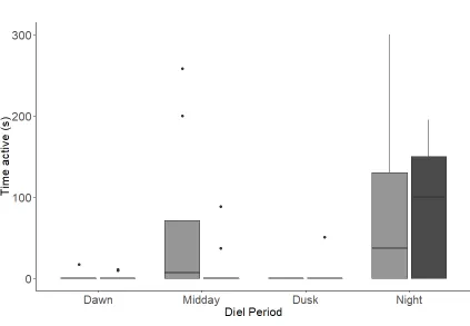
Nighttime activity level data was obtainable for the last 3 weeks for the

experiment. When night was included in the time active analysis, fish were more active

during midday and night than during dusk and dawn X2(3) = 11.20, p = 0.01; Figure 6).

During the night diel period, there was no difference in the time fish were active between

treatments (W = 32, df = 17, p = 0.72, Figure 6).

There was no association between the time active and the total invertebrate drift

(r2< 0.01, t = 1.3, df = 96, p = 0.17; Figure 7a). There was an association between time

(45)

Table 3. Generalized linear mixed models with a zero-inflated Poisson distribution

within ΔAIC of 2 from the model with the lowest AIC showing the effects of treatment,

diel period, population and the population by treatment interactions on the number of

foraging attempts of juvenile Atlantic salmon during the experiment.

Parameters Z df p AIC

Number of foraging attempts ~ Diel period 263.9

Diel period 5.00 2 < 0.001*

Number of foraging attempts ~ Diel period + Population + Treatment +

Treatment*Diel period

265.1

Diel period 4.32 2 <0.001*

Population -0.32 1 0.74

Treatment -2.41 1 0.01*

Treatment*Diel period 1.90 1 0.06

(46)

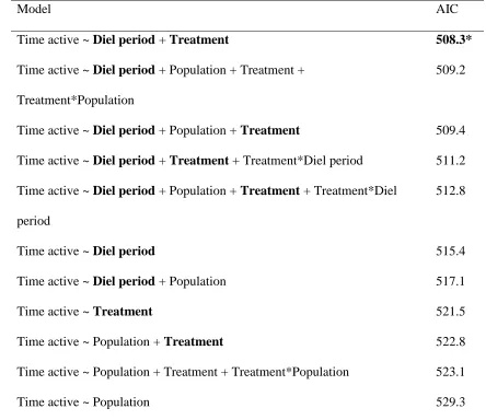
Table 4. Time active selection process using AIC. Shown are all models describing

the time active and their respective AIC.

Model AIC

Time active ~ Diel period + Treatment 508.3*

Time active ~ Diel period + Population + Treatment +

509.2

Time active ~ Diel period + Population + Treatment 509.4

Time active ~ Diel period + Treatment + Treatment*Diel period 511.2

Time active ~ Diel period + Population + Treatment + Treatment*Diel

period

512.8

Time active ~ Diel period 515.4

Time active ~ Diel period + Population 517.1

Time active ~ Treatment 521.5

Time active ~ Population + Treatment 522.8

Time active ~ Population + Treatment + Treatment*Population 523.1

Time active ~ Population 529.3

Note. Bold text indicated factor was significant according to alpha = 0.05. Asterisks

(47)

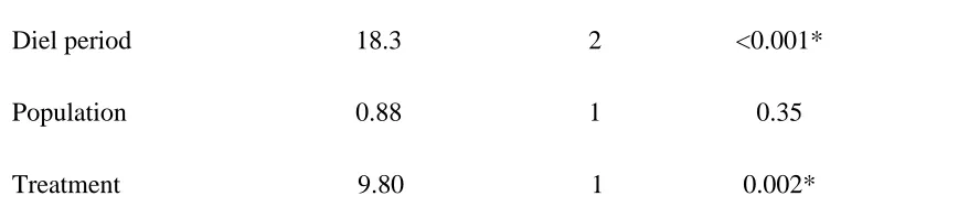
Table 5. Generalized linear mixed models with a zero-inflated Poisson distribution within ΔAIC of 2 from the model with the lowest AIC showing the effects of treatment,

diel period, population and the population by treatment interactions on the time active of

juvenile Atlantic salmon during the experiment.

Parameters X2 _df _p _AIC

Time active ~ Diel period + Population + Treatment +

509.2

Diel period 18.7 2 <0.001*

Population 0.16 1 0.68

Treatment 1.19 2 0.27

Treatment*Population 2.10 1 0.15

Time active ~ Diel period + Population + Treatment 509.4

Diel period 18.3 2 <0.001*

Population 0.88 1 0.35

Treatment 9.80 1 0.002*

(48)

A)

C))

B)

)

D)

)

E)

)

F)

(49)

Figure 5. The number of foraging attempts per observation period and time active

(seconds) of Atlantic salmon from two populations during 6-day treatments in either high

(light grey) or low shelter (dark grey) enclosures. A) The number of foraging attempts

per observation period of Atlantic salmon from the LaHave River and Sebago Lake

populations in either the high or low shelter treatments and B) Time active (seconds) of

Atlantic salmon from the LaHave River and Sebago Lake populations in either the high

and low shelter treatments. C) The number of foraging attempts per observation period of

fish in high and low shelter treatments at each diel period. and D) time active (seconds)

of fish in high and low shelter treatments at each sampling period. E) The number of

foraging attempts per observation period of fish in high and low shelter treatment over

each week and F) Time active (seconds) of fish in high and low shelter treatments over

each week. Data shown are the weekly and pen averages. Boxplots show the median, the

(50)

Figure 6. Activity level of Atlantic salmon from either high or low shelter treatments at

each diel period during 6-day treatments in either high or low shelter enclosures for the

last 3 weeks of observations. Data shown are the weekly and pen averages pooled across

populations. Boxplots show the median, the first and third quartiles, data within the

(51)

Figure 7. a) Time active (s) does not vary with food availability (r2 = 3.1 x 10-4). Shown

is a linear regression plot of activity level by total invertebrate drift rate (ln transformed).

b) Time active (s) does vary with water temperature (r2 = 0.08). Shown is a linear

regression plot of activity level by water temperature. In each panel, each point represents

data for one observation period.

Ln (total invertebrate drift rate (individuals • m-3_•_h-1₎₎

T

im

e a

c

ti

v

e (s

)

T

im

e a

c

ti

v

e (s

)

The effect of shelter availability on foraging in Atlantic salmon (Salmo salar)

Scholarship@Western

Scholarship@Western

The effect of shelter availability on foraging in Atlantic salmon

The effect of shelter availability on foraging in Atlantic salmon

(Salmo salar)

(Salmo salar)

Abstract

Keywords

Acknowledgments

Table of Contents

List of Tables

List of Figures

List of Appendices

Introduction

Predation risk and avoidance

Daily activity budgets

Population differences in foraging behaviour

Effect of predation on diet and physiological processes

Study species

Environmental influence on foraging and shelter use

Lake Ontario’s Atlantic salmon

Research Objectives and Hypotheses

Methods

Study populations

Field site and net pen design

Experimental design

Behavioural observations

Stomach content analyses

Physical parameters

Data Analyses

Results

Population differences in body size

Foraging rate, time active and number of fish foraging