Spherical Mapping of the Second-Order Phoenix Cell for Unbounded Direct Reflectarray Copolar Optimization

Vincent Richard , Renaud Loison , Raphael Gillard , Herve Legay , Maxime Romier , Jean-Paul Martinaud4, Daniele Bresciani2, and Fabien Delepaux2

Abstract—A general synthesis approach is proposed for reflectarrays using second order Phoenix cells. It relies on an original spherical representation that transforms the optimization domain in a continuous and unbounded space with reduced dimension. This makes the synthesis problem simpler and automatically guarantees smooth variations in the optimized layout. The proposed mapping is combined with an Artificial Neural Network (ANN) based behavioral model of the cell and integrated in a min/max optimization process. Bi-cubic spline expansions are used to decrease the number of variables. As an application, a contoured beam for space communication in the [3.6–4.2] GHz band is considered. The gain improvement compared to an initial Phase Only synthesis (POS) is up to 1.62 dB at the upper frequency. Full-wave simulation of the final array is provided as a validation.

1. INTRODUCTION

Passive ReflectArrays (RA) are promising antennas for applications requiring high gain, low profile, and low mass [1]. Preliminary demonstrations have been published for directive beams [2], contoured beams [3–6] or for dual-polarization [7, 8]. Most of them rely on a quite simple design process where only the phase of the main polarization at one frequency is controlled over the radiating aperture (Phase Only Synthesis, POS). Typically, this is done by selecting the geometry of each elementary cell on the reflecting panel so that it provides the desired local phase. Generally, the tuning of a single geometrical parameter is sufficient to obtain an almost 360◦ phase range and, then, a simple one-to-one correspondence between cell geometry and local phase can be established.

However, more advanced synthesis approaches [9, 10] are needed when specifications get more stringent, as for dual and multiple frequency RA or large bandwidth contoured beams for space communications. In this case, RA could advantageously compete with shaped reflectors whose fabrication is both complex and expensive. Nevertheless, their design has to address several simultaneous goals, directly at the radiation pattern level. The cell selection process is then the result of a complex trade-off. Naturally, stringent specifications also require more complex cells, with several independent geometrical parameters, in order to be able to meet the different goals. This contributes further to increased complexity. Indeed, required advanced synthesis approaches have to handle multiple goals for the array radiation by tuning multiple degrees of freedom (DoF) at each cell. For a realistic RA made of several thousands of cells, this really becomes a challenging task. On the other hand, it is believed that the successful management of this task is a key point in RA design since the availability of so many DoF may offer unique opportunity to outperform classical reflectors.

Received 23 October 2018, Accepted 10 February 2019, Scheduled 27 February 2019 * Corresponding author: Renaud Loison ([email protected]).

1 _{Institute of Electronics and Telecommunications of Rennes (IETR), UMR CNRS 6164, INSA, CS 70839, Rennes 35708, France.} 2 _{Thales Alenia Space, Toulouse 31037, France.} 3 _{Centre National des Etudes Spatiales (CNES), Toulouse 31400, France.} 4 _Thales

At this stage, a deeper insight in RA design approaches is necessary to better understand the associated challenges. As full-wave EM optimization of RA is not possible yet, design approaches usually involve a 2-step process. The first step aims at providing a full characterization of the chosen cell, by computing its complete reflection matrix [11] for any set of geometrical parameters. To do so, full-wave simulations are carried out, considering a single cell in a periodic environment (local-periodicity assumption). The resulting data is then used all along the optimization process and a very rapid access mechanism is thus essential. Most approaches rely on lookup tables with appropriate interpolating schemes [6]. Equivalent circuits can also be used [12]. Combined with filter synthesis techniques [13], they have demonstrated good capabilities for FSS [14] and even RA synthesis [15], especially regarding bandwidth optimization. Unfortunately, they are usually restricted to canonical geometries and normal incidence. Behavioral models based on Artificial Neural Networks (ANN) are more general [16, 17]. They have been used in [18] to tune the geometry of each RA cell of a narrow band RA. Here, in continuation to [19] and [20], we use 2 different ANN, one for magnitude and one for phase, in order to improve the prediction accuracy of the full reflection matrix. Efficient approaches based on ordinary kriging and support vector machines have also been proposed recently [21]. Whatever the used model, the second step in the design approach is to select the best geometry for all cells, in order to meet the specifications for the array radiation. Theoretically, this requires an iterative process in which all degrees of freedom are varied and the radiation pattern of the array is re-assessed continuously. Due to the huge number of DoF, this step is very time-consuming, even if rapid-access models are used. Here, we propose to use model-reduction techniques based on spline as it provides an efficient way to approximate a problem with a large number of DoF. This is classically done to optimize the complex geometry of shaped reflectors [22] and even the geometrical evolution of cells over RA panels [23].

Finally, it is well known [24] that successive cells must not differ too much in their geometry, and a smooth evolution has to be guaranteed all over the RA surface. This is the condition for complying with the local-periodicity assumption. To do so, an additional goal can be added in the optimization process to enforce some kind of similarity between neighbor cells [25]. However, this makes the process even more complex. Moreover, it does not prevent from the abrupt variation encountered after a complete 360◦ phase cycle has been achieved. A more relevant approach to address this issue is to use Phoenix cell. Thanks to its rebirth property [26], this cell has the unique capability to come back to its initial geometry after a complete 360◦ cycle has been reached, thus naturally preventing for any abrupt variation. Unfortunately, no RA synthesis has been reported yet, that fully takes benefit of the capabilities of the Phoenix cell. Indeed, most publications involve first order Phoenix cell [27] (i.e., with only one tuning parameter), whose capabilities are of course limited regarding multiple-purpose optimization. On the other hand, higher order Phoenix [6] cell offer additional DoF but the rebirth property is not so easy to handle since the variation domain for the geometry is now multi-dimensional. The main contribution of this paper is to propose an original spherical mapping of the second order Phoenix cell that intrinsically handles its rebirth mechanism, whatever the variation in the geometrical parameters. This mapping is associated with ANN modeling for a fast characterization of the cell. It is then integrated into an optimization process, which automatically enables to guarantee a smooth evolution of the geometry with no need to use additional constraints. Furthermore, the mapping transforms the initial optimization domain into an unbounded periodic space, and it also reduces its dimension. As a result, we arrive to a quite powerful tool dedicated to the full exploitation of the second order Phoenix cell. This is a first step before addressing the case of higher order cells with even more capabilities.

The paper is organized as follows. Section 2 is dedicated to the presentation of the spherical mapping of the second order Phoenix cell. Section 3 shows its efficient application in RA synthesis. A design example focusing on co-polarization illustrates the good performance for a 83×71 cell RA in section 4 with a full-wave simulation to valid the process. Section 5 concludes the paper.

2. A SPHERICAL MAPPING OF THE 2ND ORDER PHOENIX CELL

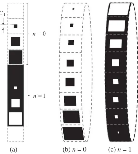
square patch with increasing size (C1). The inductive part (n= 1) is the complementary configuration

with the patch replaced by a square aperture. Figure 1(b) gives a wrapped representation of this cycle, clearly showing it provides an unbounded and continuous way of varying the geometry, as a direct consequence of the rebirth property. In the following, we refer to this cycle as a first order one since there is only one geometrical parameter (C1).

n = 0

n =1 C1

(a) (b) n = 0 (c) n = 1

Figure 1. 1D geometrical cycle of the 1st order Phoenix cell. (a) Unwrapped version. Wrapped version — (b) front side and (c) back side.

In this paper, we use the second order of this Phoenix cell by introducing a second geometrical parameter, C2. To do so, the square patch (or aperture) is replaced by a square ring, as shown in

Figure 2. The additional DoF provides more flexibility to control the reflection properties of the cell. On the other hand, it also makes trickier the management of the rebirth capabilities since this one has now to be described in a multi-dimensional space. Indeed, in order to fully benefit from the possibilities offered by the second order Phoenix cell, the representation shown in Figure 1 has to be generalized. This is the objective of the next section.

2.2. Spherical Representation of the 2nd Order Phoenix Cell

The basic rules defining this generalized representation are straightforwardly derived from those observed in Figure 1. Firstly, the representation must include all possible configurations of the cell, whatever its type (n) and its geometrical parameters (C1 and C2). Secondly, it must preserve unicity, in the

C1 C2 1 1 C1 C2 (a) (b)

Figure 2. Two different types of cells. (a) Capacitive (n= 0). (b) Inductive (n= 1).

evolution of the cell geometry all over the representation. Finally, it must not be bounded, i.e., any cell in the representation has to be surrounded by neighbors with slightly-perturbed geometries and none of them should be a stopping boundary.

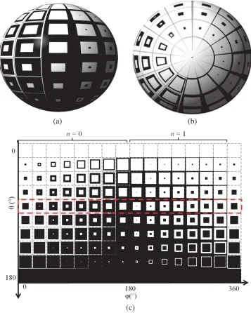
As seen in Figures 3(a) and (b), a quite natural way to define such a scheme is to use a spherical representation, similar to a world map with a 360◦ periodicity forθandφ. For the ease of understanding, Figure 3(c) also gives a planisphere version of this representation. The North and South Poles correspond to non-metallized and fully-metallized cells respectively. The 0◦and 180◦meridians match the capacitive (n= 0) and inductive (n= 1) parts of first order cycle (Figure 1). They are characterized by C2 = 0.

All other cells in the spherical representation are second order cells (C2 = 0) also defining continuous

cycles in any direction. More precisely, one parallel in the sphere is characterized by cells that all have the same metal rate. This parameter represents the percentage of metal along the length l of the cell. It continuously varies from 0% at the North Pole to 100% at the South Pole.

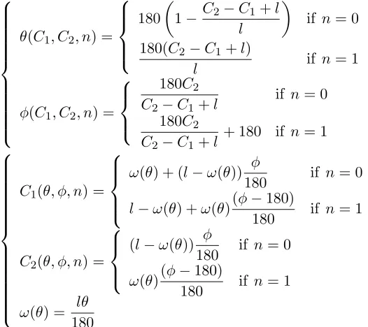
This representation scheme defines a bijective correspondence between the angular position (θ,φ), in degrees, on the sphere and the cell configuration (C1,C2,n):

⎧ ⎪ ⎪ ⎪ ⎪ ⎪ ⎪ ⎪ ⎪ ⎪ ⎪ ⎨ ⎪ ⎪ ⎪ ⎪ ⎪ ⎪ ⎪ ⎪ ⎪ ⎪ ⎩

θ(C1, C2, n) =

⎧ ⎪ ⎪ ⎨ ⎪ ⎪ ⎩ 180

1−C2−C1+l l

if n= 0

180(C2−C1+l)

l if n= 1

φ(C1, C2, n) =

⎧ ⎪ ⎨ ⎪ ⎩

180C2

C2−C1+l

if n= 0

180C2

C2−C1+l

+ 180 if n= 1

(1) ⎧ ⎪ ⎪ ⎪ ⎪ ⎪ ⎪ ⎪ ⎪ ⎪ ⎪ ⎪ ⎪ ⎪ ⎨ ⎪ ⎪ ⎪ ⎪ ⎪ ⎪ ⎪ ⎪ ⎪ ⎪ ⎪ ⎪ ⎪ ⎩

C1(θ, φ, n) =

⎧ ⎪ ⎪ ⎨ ⎪ ⎪ ⎩

ω(θ) + (l−ω(θ)) φ

180 if n= 0

l−ω(θ) +ω(θ)(φ−180)

180 if n= 1

C2(θ, φ, n) =

⎧ ⎪ ⎨ ⎪ ⎩

(l−ω(θ)) φ

180 if n= 0

ω(θ)(φ−180)

180 if n= 1 ω(θ) = lθ

180

(2)

In these equations, l is the fixed periodicity in the array.

As it will be seen in following sections, this representation proves to be particularly convenient in the RA synthesis process. Indeed, it provides a very powerful tool to deal with the tricky selection of adjacent cells when designing a RA panel. By moving over the sphere, variations in the cell configuration can be achieved with only two tuning parameters (θ and φ) in a continuous and periodic domain. Practically, this means the synthesis process can be advantageously carried out by optimizing θ and φ instead of dealing with true geometrical parameters. The interest is threefold. Firstly, the number of DoF per cell is reduced from 3 (i.e., C1,C2,n) to 2 (i.e., θ and φ). Secondly, the structure of the new

(a) (b)

(c)

Figure 3. Spherical representation with three overviews. (a) Front side view (θ= 90◦, φ = 0◦). (b) Top view (θ= 0◦ whatever φ). (c) Planisphere view.

Thirdly, unconstrained optimization is possible since the new optimization parameters are not bounded as they evolve periodically. Note that the reduction in the number of DoF per cell does not mean the solution space itself is shrunk. It is just organized in a more convenient and compact way that enforces smoothness and continuity over the RA panel. As such, it can be seen as some kind of preconditioning for the optimization process.

2.3. Spherical Mapping of the Main Characteristics

Before going into the details of the synthesis process, we show here that the spherical mapping first offers a very complete and synthetic way to observe the performance of the cell. A cell is classically characterized by its reflection matrix:

R=

RTE-TE RTE-TM

A rapid-access model is of course required to compute this matrix, whatever the geometry of the cell, the direction of the illuminating wave and the frequency. In this work, we use the ANN model we developed in [19] and [20] to predict both the phase and magnitude for all matrix coefficients. A fast assessment with high accuracy (typically 1.6◦ RMS error for the phase parameters) was demonstrated compared to full-wave simulation. Combined with the proposed spherical mapping, it enables an overview of the overall performance attainable by the chosen cell. Moreover, as the representation domain naturally guarantees smooth variations in the geometry, it directly shows whether this translates into smooth variations in the matrix coefficients themselves.

As an example, Figure 4 presents the mapping of the RTE-TE phase calculated using the ANN

model over the sphere for all possible cell configurations. The studied cell is printed on a Honeycomb substrate with thickness h = 20 mm, dielectric constant = 1.03 and loss tangent tanδ = 0.003. The periodicity isl= 25.6 mm (λ/3 at 3.9 GHz). The mapping is carried out at normal incidence and for 3 different frequencies. In order to better see the transition in the phase when moving from a capacitive cell to an inductive one (or conversely), the φ angle in the planisphere mapping is varied from 0◦ to 385◦. In other words, the [360◦,385◦] interval on the right of the plot is a repetition of the [0◦,25◦] interval on the left.

The first output from this plot is that any phase value from−180◦to 180◦can be reached by the cell. Moreover, most of them can be obtained with several different geometries, which provides additional flexibility in the synthesis process. Globally, the plot also shows the phase variations are quite regular. However, one can detect a slight discontinuity (less than 15◦) when moving from a capacitive to an inductive cell (atφ= 180◦) and a more significant one (up to 50◦) when passing the converse transition (atφ= 360◦). An optimal trajectory on the sphere would be a closed path passing through all possible phase values while minimizing the discontinuities when nis changed. A closer examination of the plot shows it is achieved by choosing the equator (dotted line in Figure 4(b)). This results from the fact that the discontinuity at the first transition (φ= 180◦) gets higher when approaching the South Pole while that at the second transition (φ = 360◦) becomes larger close to the North pole. The RTE-TE phase

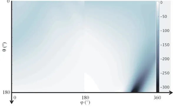
evolution (atf = 3.9 GHz) along this equatorial cycle is presented in Figure 5. As we will see later on, this trajectory will play an important role when choosing the initial conditions for the synthesis process. Finally, the modification of the plot versus frequency is an indicator about dispersion, described in Eq. (4) in ◦/GHz. A more direct information is given by Figure 6 that plots phase dispersion over the bandwidth. It confirms each phase value can be obtained with various possible dispersion levels. The minimum value, 0◦/GHz, is obtained close to the South Pole where the fully-metallized cell is equivalent to a PEC boundary. The maximum value (absolute value), 340◦/GHz, is obtained in the back area, where a resonant phenomenon associated with large and narrow slot-rings is encountered.

ΔΦTE-TE

Δf =

Φ_fmax −Φ_fmin fmax−fmin

(4)

3. OPTIMIZATION ALGORITHM 3.1. Goal and Used Cost Function

In the context of space antennas, the goal of the RA optimization process can be to reach an objective radiated field Eobj associated with a defined coverage on Earth. This field is specified at Nsta station

distributed over the Earth and at Nfreq frequencies f in a given band. To this aim, a min/max

optimization process is used [30]. For example, in the case of a co-polar optimization, the cost function is defined as the maximum of the difference between the co-polar components of the objective field and the field Erad radiated by the RA under optimization:

= max f max k _Eobj

co (k, f)−Ecorad(k, f)

(5)

withk= 1, . . . , Nsta. In the optimization process,Erad is calculated using geometrical optics where the

(a) 3.6 GHz

(b) 3.9 GHz

(c) 4.2 GHz

Figure 4. RTE-TE phase (degrees) on the spherical representation and at different frequencies.

3.2. Optimization DoF and Initial Condition

As already mentioned, we propose to optimize the RA panel directly on theθandφparameters instead of the true geometrical ones (C1,C2,n). For a RA constituted ofNx and Ny cells alongx and y axes

respectively, the array is entirely defined by θij and φij for i ∈ [1, Nx] and j ∈ [1, Ny]. The initial number of DoF is thus given by:

NDoFinit = 2NxNy (6)

Figure 5. RTE-TE phase evolution along the equatorial cycle at the central frequency 3.9 GHz.

Figure 6. Dispersion over the bandwidth of the RTE-TE phase (degrees/GHz) on the spherical

representation and at the central frequency 3.9 GHz.

To vary θij and φij from the initial layout within the optimization process, Δθij and Δφij are

introduced:

θij =θ_ij0 + Δθij

φij =φ0_ij + Δφij (7)

Δθij and Δφij are the newNDoF_init parameters to be optimized. For space applications,NDoF_init can be

huge reaching up to several thousands. For computation time and convergence reasons, the complexity is reduced by expanding the unknowns on approximation functions so that the required information is compressed without sacrificing accuracy:

⎧ ⎪ ⎪ ⎪ ⎪ ⎪ ⎨ ⎪ ⎪ ⎪ ⎪ ⎪ ⎩

Δθij = NSx

l=1

cx_lS_lx(xi) NSy

m=1

cy_mS_my(yj)

Δφij = NSx

l=1

dx_lS_lx(xi) NSy

m=1

dy_mS_my(yj)

NDoF = 2NSxNSy (9)

Strictly speaking, this is not really a reduction in the number of available DoF but a compressed representation of them.

3.3. Optimization Algorithm

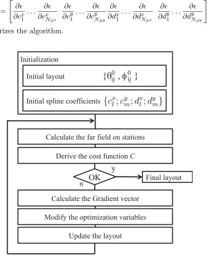
Based on the min/max algorithm, the objective is to minimize the cost function (Eq. (5)) by modifying the spline coefficients. To achieve this, an off-the-shelf conventional iterative gradient descent is used. In order to get the best orientation in the DoF space, the following gradient vector G is calculated numerically at each iteration:

G=

∂ ∂cx1

. . . ∂ ∂cx_NSx

∂ ∂cy1

. . . ∂ ∂cy_NSy

∂ ∂dx1

. . . ∂ ∂dx_NSx

∂ ∂dy1

. . . ∂ ∂dy_NSy

(10)

Figure 7 summarizes the algorithm.

Initialization

Initial layout

Initial spline coefficients

Modify the optimization variables

Update the layout Calculate the far field on stations

Derive the cost function C

Calculate the Gradient vector

OK

y

{

θ

,

φ

}

4. APPLICATION TO A C-BAND MISSION 4.1. Mission Specifications

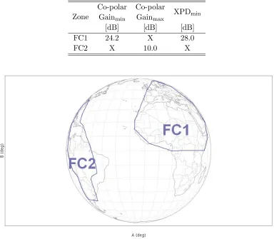
To illustrate the algorithm performances, we consider a C-band space telecommunication mission. The coverage zones are shown in Figure 8 and the co-polarization (co-polar) gain and cross-polarization discrimination (XPD) requirements are summarized in Table 1. The purpose of the mission is to provide service to Europe, North Africa and Middle East (FC1 zone) while minimizing illumination in South America (FC2 zone). The antenna operates in left-handed circular polarization in the limited transmission C-band [3.6, 4.2] GHz.

Table 1. Coverage requirements.

Zone

Co-polar Co-polar

XPDmin

Gainmin Gainmax

[dB] [dB] [dB]

FC1 24.2 X 28.0

FC2 X 10.0 X

Figure 8. Coverage zones of the telecommunication mission. FC1: co-polar directivity. FC2: co-polar isolation.

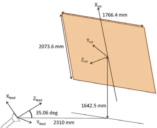
4.2. Antenna and Optimization Parameters

This work concerns only the layout design, and the antenna system parameters such as the feeding antenna type and position and the RA dimensions are fixed and given in Figure 9.

The RA panel is 28λ along x and 24λ along y at the central frequency f = 3.9 GHz. The array periodicity is λ/3 along x and y resulting in Nx = 83 and Ny = 71 RA cells, the initial number of optimization DoF is thus NDoF_init = 11786.

Figure 9. Fixed antenna architecture.

number of optimization DoF is then NDoF = 800. Nsta is set to 300 station points with a uniform

distribution in the zone of interest.

In this paper, the developed mapping is restricted to the 2nd order cell. Such a cell intrinsically offers no simple means of controlling cross-polar because it has a square symmetric geometry. Then in this example, we decided to focus only on co-polarization and try to optimize it on a quite large bandwidth (16%). Consequently, no goal was given for the cross.

Introducing new geometrical parameters, XPD could be optimized as it is done in [34] by converting square Phoenix cells into rectangular ones or by the use of parallelogram or trapezoid shaped elements as in [31]. Cross-polarization could also theoretically be optimized at the array level with symmetrical cells [35]. Once again, this was not possible here as all available DoF were already necessary to address the co-polar specifications (for both the illuminated and isolated zones) over the bandwidth.

4.3. Initial Layout

The required co-polarization phase distribution on the RA at the central frequency f = 3.9 GHz is presented in Figure 10. Using the equator cycle and its one-to-one correspondence between cell geometry and reflected co-polar phase, the initial layout is easily designed. As shown in Figure 11, this layout presents smooth geometrical variations. This property tends to respect the expected local periodicity for the cells.

The simulated radiation patterns of the initial layout are presented in Figure 12(a), and the achieved performances are synthesized in Table 2. As expected, the performances respect the specifications only at the central frequencyf = 3.9 GHz and for the radiated co-polar.

4.4. Optimization Run

Figure 10. Ideal RTE-TE phase (degrees)

requirement at 3.9 GHz.

Figure 11. Initial layout for the C-band mission.

(a1) 3.6 GHz (a2) 3.9 GHz (a3) 4.2 GHz

(b1) 3.6 GHz (b2) 3.9 GHz (b3) 4.2 GHz

Figure 12. Simulated radiation pattern in co-polarization gain [dBi] for left polarization at different frequencies. (a) Initial RA. (b) Optimized RA.

calculate gradients given by Eq. (10)). Such improvements were not addressed in this study, whose main scope was the spherical mapping.

FC2 X 6.7 X

4.2 FC1 22.7 X 21.95

FC2 X 7.84 X

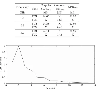
Table 3. Optimized RA performances.

Frequency

Zone

Co-polar Co-polar

XPDmin

Gainmin Gainmax

GHz [dB] [dB] [dB]

3.6 FC1 24.65 X 22.52

FC2 X 7.62 X

3.9 FC1 24.28 X 22.09

FC2 X 6.46 X

4.2 FC1 24.14 X 20.25

FC2 X 7.43 X

0 2 4 6 8 10 12 14

iteration

0 0.5 1 1.5 2 2.5 3

Cost function

Figure 13. Convergence of the cost function.

4.5. Validation by Full-Wave Simulation

For validation purpose, a full-wave simulation of the whole antenna system is proposed in this section. A homemade solver based on integral equations in frequency domain is used [36]. Figure 14 shows the comparison between the full-wave solver results and the one obtained with array theory under local periodicity assumption.

It must be highlighted that the agreement is very good. This definitely shows that the reached geometrical continuity over the panel is a key point to comply with the local periodicity assumption. Thanks to that, conventional array theory can be used with confidence in the optimizing process.

Figure 14. Comparison of radiation patterns obtained with full-wave solver (blue curves) and homemade analytical tool (red curves) at 3.9 GHz.

5. CONCLUSION

This paper describes an original spherical mapping for the 2nd order Phoenix cell. It appears as an essential tool to fully benefit from this versatile but complex cell. It first provides a convenient way to visualize its overall properties. Moreover, it leads to an optimization domain that directly inherits its continuous and cyclic evolution. This makes it fully suitable with spline that leads to a compressed formulation of the problem to be optimized. In this paper, the mapping is combined with ANN modeling and encapsulated in a min/max optimization process, thus resulting in a general optimization package. It is successfully applied to optimize a contoured beam coverage for space communication on a 16% frequency bandwidth. The gain at the upper frequency is improved by 1.62 dB compared to the initial POS. The excellent agreement with full-wave simulation confirms that the proposed methodology automatically generates a regular RA layout that naturally complies with the implicit local-periodicity assumption.

applications,” IEEE Transactions on Antennas and Propagation, Vol. 52, No. 5, 1138–1148, May 2004.

5. Zhou, M., S. B. Sorensen, R. Jorgensen, O. Borries, E. Jorgensen, and G. Toso, “High-performance curved contoured beam reflectarrays with reusable surface for multiple coverages,” 2017 11th

European Conference on Antennas and Propagation (EUCAP), 71–75, Mar. 2017.

6. Legay, H., D. Bresciani, E. Labiole, R. Chiniard, R. Gillard, and G. Toso, “Measurement of a 1.3 m reflectarray antenna in at panels in ku band,” 2012 International Symposium on Antennas and Propagation (ISAP), 231–234, Oct. 2012.

7. Hasani, H., C. Peixeiro, A. K. Skrivervik, and J. Perruisseau-Carrier, “Single-layer quad-band printed reflectarray antenna with dual linear polarization,” IEEE Transactions on Antennas and Propagation, Vol. 63, No. 12, 5522–5528, Dec. 2015.

8. Florencio, R., J. A. Encinar, R. R. Boix, V. Losada, and G. Toso, “Reflectarray antennas for dual polarization and broadband telecom satellite applications,” IEEE Transactions on Antennas and Propagation, Vol. 63, No. 4, 1234–1246, Apr. 2015.

9. Bucci, O. M., A. Capozzoli, G. D’Elia, and S. Musto, “A new approach to the power pattern synthesis of reflectarrays,” Proc. URSI International Symposium on Electromagnetic Theory (EMTS’04), 1053–1055, 2004.

10. Zhou, M., S. B. Srensen, O. S. Kim, E. Jrgensen, P. Meincke, and O. Breinbjerg, “Direct optimization of printed reflectarrays for contoured beam satellite antenna applications,” IEEE Transactions on Antennas and Propagation, Vol. 61, No. 4, 1995–2004, Apr. 2013.

11. Wan, C. and J. A. Encinar, “Efficient computation of generalized scattering matrix for analyzing multilayered periodic structures,” IEEE Transactions on Antennas and Propagation, Vol. 43, No. 11, 1233–1242, Nov. 1995.

12. Al-Joumayly, M. A. and N. Behdad, “A generalized method for synthesizing low-profile, band-pass frequency selective surfaces with non resonant constituting elements,” Int. Journal of Antennas and Propag., Vol. 58, No. 12, 4033–4041, Dec. 2010.

13. Liang, L. and S. V. Hum, “An impedance surface-based method for designing wideband reflectarrays,”2015 IEEE Int. Sym. on Ant. and Propag. USNC/URSI Nat. Radio Science Meeting, 2135–2136, Jul. 2015.

14. Zhou, M., S. B. Sorensen, N. Vesterdal, R. Dickie, P. Baine, J. Montgomery, R. Cahill, M. Henry, P. G. Huggard, and G. Toso, “Design of aperiodic frequency selective surfaces for compact quasioptical networks,”2017 11th European Conference on Antennas and Propagation (EUCAP), 1274–1278, Mar. 2017.

15. Hum, S. V. and B. Du, “Equivalent circuit modeling for reflectarrays using oquet modal expansion,”

IEEE Transactions on Antennas and Propagation, Vol. 65, No. 3, 1131–1140, Mar. 2017.

16. Robustillo, P., J. Zapata, J. A. Encinar, and J. Rubio, “Ann characterization of multi-layer reflectarray elements for contoured-beam space antennas in the ku-band,” IEEE Transactions on Antennas and Propagation, Vol. 60, No. 7, 3205–3214, Jul. 2012.

17. Freni, A., M. Mussetta, and P. Pirinoli, “Neural network characterization of reflectarray antennas,”

18. Robustillo, P., J. Zapata, J. A. Encinar, and M. Arrebola, “Design of a contoured-beam reflectarray for a eutelsat european coverage using a stacked-patch element characterized by an artificial neural network,” IEEE Antennas and Wireless Propagation Letters, Vol. 11, 977–980, 2012.

19. Richard, V., R. Loison, R. Gillard, H. Legay, and M. Romier, “Optimized artificial neural network for reflectarray cell modelling,”2016 IEEE International Symposium on Antennas and Propagation (APSURSI), 1211–1212, Jun. 2016.

20. Richard, V., R. Loison, R. Gillard, H. Legay, and M. Romier, “Loss analysis of a reflectarray cell using anns with accurate magnitude prediction,”2017 11th European Conference on Antennas and Propagation (EUCAP), 2396–2399, Mar. 2017.

21. Salucci, M., L. Tenuti, G. Oliveri, and A. Massa, “Efficient prediction of the em response of reflectarray antenna elements by an advanced statistical learning method,”IEEE Transactions on Antennas and Propagation, Vol. 66, No. 8, 3995–4007, Aug. 2018.

22. Engineering Consultants, POS,User’s Manual, TICRA, 2001.

23. Zhou, M., S. B. Srensen, E. Jrgensen, and P. Meincke, “Efficient optimization of large reflectarrays using continuous functions,” 2013 7th European Conference on Antennas and Propagation (EuCAP), 2952–2956, Apr. 2013.

24. Milon, M. A., R. Gillard, D. Cadoret, and H. Legay, “Analysis of mutual coupling for the simulation of reflectarrays radiating cells,”2006 First European Conference on Antennas and Propagation, 1–6, Nov. 2006.

25. Marnat, L., R. Loison, R. Gillard, D. Bresciani, and H. Legay, “Comparison of synthesis strategies for a dual-polarized reflectarray,” Int. Journal of Antennas and Propag., Vol. 2012, Article ID 708429, 10 pages, 2012.

26. Moustafa, L., R. Gillard, F. Peris, R. Loison, H. Legay, and E. Girard, “The Phoenix cell: A new reflectarray cell with large bandwidth and rebirth capabilities,”IEEE Antennas and Wireless Propagation Letters, Vol. 10, 71–74, 2011.

27. Makdissy, T., R. Gillard, E. Fourn, M. Ferrando-Rocher, E. Girard, H. Legay, and L. Le Coq, “Phoenix: Reflectarray unit cell with reduced size and inductive loading,” IET Microwaves Antennas Propagation, Vol. 10, 1363–1370, 2016.

28. Salti, H. and R. Gillard, “A single layer stub-patch phoenix cell for large band reflectarrays,”2017 11th European Conf. on Ant. and Propag., 2405–2408, Mar. 2017.

29. Zhang, K., Y. Fan, J. Xu, and C. Qu, “Design of broadband, low cost single layer reflectarray using phoenix cell,” 2013 IEEE International Conference of IEEE Region 10 (TENCON 2013), 1–4, Oct. 2013.

30. Hald, J. and K. Madsen, “Combined lp and quasi newton methods for minimax optimization,”

Math. Programming, Vol. 20, 49–62, 1981.

31. Legay, H., D. Bresciani, E. Labiole, R. Chiniard, and R. Gillard, “A multi facets composite panel reflectarray antenna for a space contoured beam antenna in ku band,”Progress In Electromagnetics Research, Vol. 54, 1–26, 2013.

32. Encinar, J. A., M. Arrebola, L. F. de la Fuente, and G. Toso, “A transmit-receive reflectarray antenna for direct broadcast satellite applications,” IEEE Transactions on Antennas and Propagation, Vol. 59, No. 9, 3255–3264, Sept. 2011.

33. De Boor, C.,A Practical Guide to Splines, Vol. 27, Springer-Verlag New York, 1978.

34. Zhou, M., O. Borries, and E. Jrgensen, “Design and optimization of a single-layer planar transmitreceive contoured beam reflectarray with enhanced performance,” IEEE Transactions on Antennas and Propagation, Vol. 63, No. 4, 1247–1254, Apr. 2015.

35. Encinar, J. A. and M. Arrebola, “Reduction of cross-polarization in contoured beam reflectarrays using a three-layer configuration,” 2007 IEEE Antennas and Propagation Society International Symposium, 5303–5306, IEEE, 2007.