An Efficient Combination of Dispatch Rules for
Job-shop Scheduling Problem
Tatsunobu Kawai, Yasutaka Fujimoto
Department of Electrical and Computer Engineering, Yokohama National University, Yokohama 240-8501 JAPAN [email protected],[email protected]
http://www.fujilab.dnj.ynu.ac.jp
Abstract— This paper present new combinations of
dis-patch scheduling for Job Shop Scheduling Problem. The
Job Shop Scheduling Problem is one of the NP hard
op-timization problems, and it is difficult to obtain the exact optimal solution. Scheduling methods based on the dispatch
rule are a set of efficient approximate methods. In this
pa-per, by combining several dispatch rules, we have proposed
three new rules. The first rule is the rule that combines
two simple dispatch rules which are often adopted in actual production systems. The proposed rule gives better result than that of any single dispatch rule. The second rule is the rule that keeps balance of remaining load of all machines. In this rule, the weight is decided in early stage of the sched-ule. It gives good solutions with high probability. The third rule is the rule that predetermines the mixing ratio, which accompanies a sequence of operations. This rule often gives better results than any other dispatch rules.
I. Introduction
In recent years, multi-item small-lot-sized production be-comes popular since it is possible to meet wide variety of consumer needs and shortened life cycle of goods. A scheduling problem for this type of production system be-comes very complex.
Many real scheduling problems are represented as Job Shop Scheduling Problem (JSSP). Because almost all scheduling problems, comprising JSSP, are the NP hard optimization problem, an efficient approximate method is required. The approximate methods are categorized in heuristics and meta-heuristics. Meta-heuristics are meth-ods that search many solutions simultaneously by sim-ple calculation and choose the best one in the solutions. This category includes Genetic-Algorithm and Simulated-Annealing.
Heuristics depend on experience and expertise like dis-patch rules. Since the disdis-patch rules are based on expe-rience and expertise, some of the dispatch rules are not effective for some problems, i. e., conventionally, there is no dispatch rule that always gives good solution for any problem. Therefore, it is useful to develop a new rule that can be applied to many problems. A survey of dis-patch rules is found in [1].
In this paper, by combining several dispatch rules, we propose a new rule that can give shorter makespan than that of other general dispatch rules for many problems.
II. Conventional Dispatch Rules
A. Conventional Dispatch Rules
The below list shows various type of conventional dis-patch rules. These rules are widely adopted at many fac-tories .
• SPT (Shortest Processing Time)
– select a job which has the shortest processing time
• LPT (Longest Processing Time)
– select a job which has the longest processing time
• MWKR (Most WorK Remaining)
– select a job which has longest total processing time remaining
• LOPN (Least OPeration Numbers)
– select a job which has the least operation number
• SLACK
– select a job which has the shortest due date
Our new scheduling method is based on these dispatch rules.
B. Dependence of Rules on Properties of Problems
An effectiveness of a dispatch rule tends to depend on characteristics of structure of problems. Although this fact has not been theoretically discussed well in past works, it is generally understood to be possible. In order to develop a new combination of the rules, it is effective to investigate how each dispatch rule depends on properties of the problems.
In numerical simulations, we adopt four dispatch rules for thirteen bench mark problems which are given by the OR-Library[2]. The OR-Library is a collection of test data sets for a variety of Operations Research (OR) problems these bench mark problems are regarded as representatives of the JSSP.
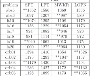
The simulation results are shown in Table I. In the Ta-ble I, a mark “**” denotes the shortest makespan among the four rules. From the Table I, MWKR gives many good and stable makespans than the other three rules. SPT and LOPN give some good makespans. On the other hand, LPT gives worse makespans. The Table I shows that the effective rule differs depending on properties of the prob-lems.
C. Sensitivity of Rules
When two or more dispatch rules are combined and different priorities are mixed together, a top prior job under
TABLE I
Makespan of each dispatch rules
Rule problem SPT LPT MWKR LOPN abz5 **1352 1586 1369 1356 abz6 1097 1207 **987 989 ft10 **1074 1295 1108 1179 la16 1156 1229 **1054 1173 la17 924 1082 **846 928 la18 981 1114 **970 972 la19 **940 1062 1013 975 la20 1000 1272 **964 1160 orb01 1394 1410 1354 **1326 orb02 1175 1293 **1047 1157 orb03 **1179 1430 1247 1404 orb04 1236 1427 1172 **1132 orb05 1128 1099 1173 **1055
the mixed dispach rule may differ from top prior jobs under the original dispach rules. Namely, from the viewpoints of the original priorities, a less prior job can be selected. In this section, we investigate the makespan for the case that a machine selects a job of second priority only once under a single dispach rule. This analysis shows a sensitivity of a single dispach rule. If the makespan varies much, we can say that rule is sensitive to the priority. In this case, the selection of a less prior job may yield improvement of the makespan.
Various scenario are tested for the problem ft10 us-ing four dispach rules SPT, LPT, MWKR, and LOPN. There are many conflicting points during scheduling, that is, a second prior job is selected once at a randomly se-lected stage of scheduling. The histogram in Fig. 1 shows the number of realizations falling into each ranges of makespans. Results using usual priority are also shown in Table I. From Fig. 1, the variances of the makespan of SPT and LOPN are small. On the other hand, and MWKR has the large variance. As the result, it is possible to improve the makespan by introducing an other priority attribute in addition to the basic rule.
III. Combination of Rules
A. Proposed Method I
Since a processing sequence of the conventional dispatch schedule is decided by the simple priority rule, there is no general rule for every scheduling problem. Therefore, it is useful to develop a combined rule that gives more flexible and better results to many problems.
In this paper, we propose a novel rule based on a com-bination of some dispatch rules. From Fig. 1, we can im-prove the schedule and the makespan by selecting a job of lower priority in some cases. Combination of some dis-patch rules changes criterion of the priority. Therefore, using a combined rule can shorten the makespan, and the combined rule can be applied to many scheduling problems when a proper weight of each rules is selected. We propose
0 2 4 6 8 10 12 14 16 18 20 22 24 26 28 30 32 1000 1100 1200 1300 1400 1500 1600 Number(number) Makespan(h) SPT LPT LOPN MWKR
Fig. 1. Distribution of makespan when a second priority job is se-lected only once (ft10)
a method to determine weight of each rule in early stage during the scheduling.
A.1 SPT and SLACK
From the results of previous section, SPT and MWKR are selected as candidates for the combination of rules. Ac-tually we adopt SPT and SLACK. SLACK can give the same result as MWKR when all jobs have a same due date. The proposing rule is defined as
min
j Skj =h1pkj+ (1−h1)
sj
Jk, (1)
0< h1<1,
where pkj denotes processing time of job j in machinek
andsj is SLACK of job j defined as
sj =dj−lj−t, (2)
wheredjdenotes a due date of jobj,ljdenotes a remaining processing time of job j, and t is a present time, respec-tively. Jk denotes a number of remaining jobs of machine k. For machine k, this combination of rules of SPT and SLACK selects a job that has the smallest Skj. We call this rulemethod I.
A.2 Simulation of Method I
To confirm the effectiveness of the method I, we exam-ined the makespan when parameterh1 changes from 0 to
1.
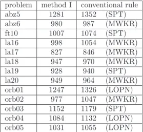
Thirteen bench mark problems[2] are adopted for the simulations. Due dates are set for all of these problems. The simulation results are shown in Fig. 2 and Table II. In Table II, conventional rule means the shortest makespan among the four rules (SPT, LPT, MWKR and LOPN). In Fig. 2, 5/10, 7/10, 9/10 mean the corresponding lap time of processing. For example, 5/10 is the time when a half of total process is finished.
From Table II, the combined rule gives the best result in all problems, when a proper parameterh1 is given.
From Fig. 2, the proper parameterh1changes depending
300 400 500 600 700 800 900 1000 1100 0 0.2 0.4 0.6 0.8 1 Time(h) h1(number) Makespan 9/10 7/10 5/10
Fig. 2. Parameterh1 v.s. processing time (la18)
TABLE II Makespan of method I
problem method I conventional rule abz5 1281 1352 (SPT) abz6 980 987 (MWKR) ft10 1007 1074 (SPT) la16 998 1054 (MWKR) la17 827 846 (MWKR) la18 947 970 (MWKR) la19 928 940 (SPT) la20 949 964 (MWKR) orb01 1247 1326 (LOPN) orb02 977 1047 (MWKR) orb03 1152 1179 (SPT) orb04 1084 1132 (LOPN) orb05 1031 1055 (LOPN)
best result when 9/10 of the schedule have been completed. However, it finally gives the worst makespan. The reason is that the remaining jobs collect to a certain machine. In order to decide the parameterh1in early stage of schedule,
it is expected that we need to keep a balance of remaining operation time of all machines.
B. Proposed Method II
To keep remaining loads in all machines balanced, a new factor is introduced.
B.1 Uniform Job Remaining
To keep a balance of remaining operation time of all machines, the following indexUjis introduced. A job with
leastUj should be selected for machine k. Uj is defined as Ukj=˛˛˛˛(lk−pkj)−l1+l2+· · ·+ (lk−pkj) +· · ·+lm
m
˛˛ ˛˛, (3)
wherelk denotes a remaining operation time of a machine k and pkj denotes a processing time of job j in machine k, respectively. This attribute is named UJR (Uniform Job Remaining) in this paper. The combination of rules of
TABLE III
Makespan of method II (10 job 10 machine)
mean (variance) problem 10/10 3/10 5/10 abz5 1281 1308 (5.3) 1334 (0.0) abz6 980 980 (0.0) * 991 (15.8) ft10 1007 1020 (5.2) 1020 (5.2) la16 998 *1148 (33.2) *1144 (61.8) la17 823 834 (15.6) 836 (0.0) la18 907 * 985 (15.1) * 993 (6.6) la19 896 *1002 (22.9) * 994 (1.4) la20 949 *1023 (76.4) 949 (0.0) orb01 1196 1246 (41.8) 1196 (0.0) orb02 921 978 (24.0) 1016 (0.0) orb03 1147 *1194 (11.2) *1194 (11.2) orb04 1084 *1252 (32.2) *1233 (6.7) orb05 1015 *1065 (18.2) *1097 (10.6)
UJR, SPT and SLACK is again represented by min
j Skj =h1pkj+h2
sj
Jm+ (1−h1−h2)Uj, (4)
0< h1<1, 0< h2<1, h1+h2<1.
In this rule, we select a job with the smallestSkj. This is a proposedmethod II.
B.2 Simulation of Method II-1
We examined the best makespan whenh1andh2change from 0 to 1. Then we examined the best combination of
h1 and h2 at 3/10 and 5/10 of the total processing time.
After fixingh1andh2, the rest of schedule is planned. The
mean and the variance of the makespan are calculated for all conflicting schedules.
Table III shows the best makespan of the combined rule, the mean and the variance of the makespan with the best combination of h1 and h2 at the stage of 3/10 and 5/10.
The mark “*” denotes the mean of the makespan is longer than the conventional rule in Table II.
From Table III, many problems have the mark “*”. It means that it is difficult to decide h1 and h2 in the early
phase for small scale problems. B.3 Simulation of Method II-2
Table IV presents simulation results for large scale prob-lems with 100-job-100-machine. Other conditions are same as the case of the simulation of Method II-1. In this ta-ble, data5 to data16 are problems in which sequence of operations for each job are random. data21 to data30 are problems in which sequence of operations for each job are similar.
From Table IV, while a number of the mark “*” is fewer than Table III, some problems still have the mark, i. e., it is still difficult to decideh1andh2in early stage of the
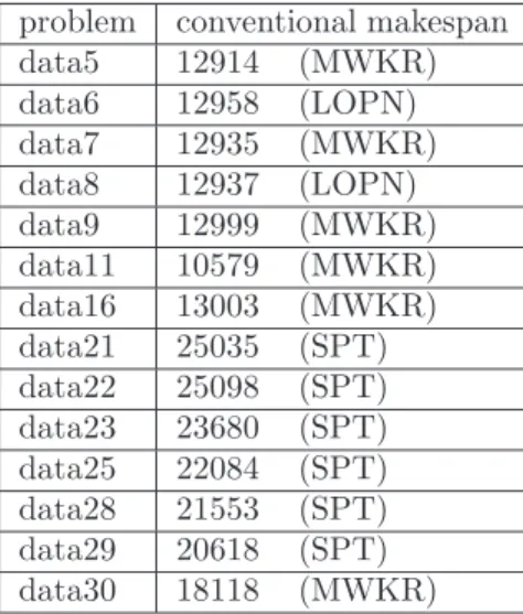
sched-ule. In addition, results of similar sequence problems are worse than results of random sequence problems. Table V shows conventional makespans of same problems. MWKR
TABLE IV
Makespan of method II-1 (100-job-100-machine)
mean (variance) problem 10/10 3/10 5/10 data5 12551 12643 (52.6) 12639 (0.0) data6 12613 12767 (0.0) 12834 (0.0) data7 12531 12740 (36.8) 12545 (0.0) data8 12603 12783 (0.0) 12687 (0.0) data9 12650 12966 (23.0) 12709 (0.0) data11 10183 10254 (41.5) 10514 (0.0) data16 12733 12904 (0.0) 12864 (0.0) data21 24054 24192 (144.7) 24149 (0.0) data22 24668 *25961 (149.0) 24815 (19.3) data23 23473 *25030 (0.0) *24723 (0.0) data25 21271 *23973 (0.0) 21518 (0.0) data28 20400 *21882 (0.0) 21031 (525.4) data29 19976 *21119 (0.0) 20299 (84.3) data30 16682 17245 (0.0) 17111 (0.0) TABLE V Conventional makespan
problem conventional makespan data5 12914 (MWKR) data6 12958 (LOPN) data7 12935 (MWKR) data8 12937 (LOPN) data9 12999 (MWKR) data11 10579 (MWKR) data16 13003 (MWKR) data21 25035 (SPT) data22 25098 (SPT) data23 23680 (SPT) data25 22084 (SPT) data28 21553 (SPT) data29 20618 (SPT) data30 18118 (MWKR)
tends to give good results for random sequence problems and SPT tends to give good results for similar sequence problems.
B.4 Effect of Processing Sequence
It is effective to apply SPT rule for early scheduled chines and to apply SLACK rule for late scheduled ma-chines. LetAk be an index of earliness of processing order
in operations in machinek. Ak is defined as
Ak =−(Rk−RAV E)Mktk
MAV E , (5)
whereRkdenotes the average processing order in machine kfor all jobs. RAV Edenotes the average of allRk. Mk de-notes the number of remaining operations in machinek. tk
denotes the average processing time of operations in ma-chinek for all jobs. Ak >0 means the average processing
order in machinekis early, andAk<0 means the average
TABLE VI
Makespan of method II-2 (100-job-100-machine)
mean (variance) problem 10/10 3/10 5/10 data5 12557 12646 (57.3) 12646 (57.3) data6 12656 12805 (0.0) 12841 (0.0) data7 12601 12698 (78.3) 12834 (62.9) data8 12597 12737 (0.0) 12736 (89.7) data9 12651 12886 (0.0) 12686 (46.4) data11 10174 10292 (25.2) 10234 (11.0) data16 12804 12929 (5.2) 12952 (0.0) data21 24255 24515 (246.8) 24439 (227.3) data22 25023 *26098 (239.3) 25017 (0.0) data23 23515 *23964 (192.8) *23902 (46.1) data25 21460 22038 (90.4) 21962 (84.6) data28 20484 20978 (0.0) 20978 (0.0) data29 20275 20607 (147.2) *20645 (166.7) data30 17022 17617 (270.9) 17744 (31.9)
processing order in machine kis late. The modified UJR rule considering the new factorAk is defined as
U
j=˛˛˛˛(lk−pj)−(l1+l2+· · ·+ (lk−pj) +· · ·+lm
m −Ak)
˛˛ ˛˛. (6)
Due to the factorAk, if the average order in machinek
is early, SPT is preceded. If the average order in machine
kis middle,Ak has a small value.
Table VI presents the result of the combined rule Uj.
By comparing Table IV with Table VI, a number of the mark “*” is fewer than Table IV. Decrease of the mark “*” means an improvement in a combined rule. Therefore, this combined rule can give good results by determining the parameterh1 andh2 in early stage of the schedule.
C. Proposed Method III
From Table V, it is clear that MWKR is effective in random sequence problems, and SPT is effective in similar sequence problems. We propose the third combined rule that predetermine the parameterh1as follows.
C.1 Predetermination of Weight of Rules In a proposed method III,h1 is given by
h1= Rk/RAV E
2 . (7)
Ifh1 is bigger than 1/2, SPT becomes dominant. Other-wise, SLACK becomes dominant.
C.2 Simulation of Method III
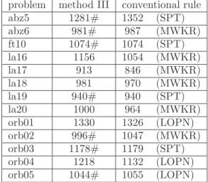
Table VII and Table VIII present the result of the pro-posed method III for 10-job-10-machine and 100-job-100-machine problems. In this table, a mark “#” denotes that the makespan of the proposed method III is better than the best among the conventional four rules.
The proposed method III yields better makespans for 12 problems out of 27 problems, i. e., the method is more
TABLE VII
Makespan of method III (10 job 10 machine)
problem method III conventional rule abz5 1281# 1352 (SPT) abz6 981# 987 (MWKR) ft10 1074# 1074 (SPT) la16 1156 1054 (MWKR) la17 913 846 (MWKR) la18 981 970 (MWKR) la19 940# 940 (SPT) la20 1000 964 (MWKR) orb01 1330 1326 (LOPN) orb02 996# 1047 (MWKR) orb03 1178# 1179 (SPT) orb04 1218 1132 (LOPN) orb05 1044# 1055 (LOPN) TABLE VIII
Makespan of method III (100 job 100 machine)
problem method III conventional rule data5 12728# 12914 (MWKR) data6 12969 12958 (LOPN) data7 12864# 12935 (MWKR) data8 13390 12937 (LOPN) data9 13107 12999 (MWKR) data11 10980 10579 (MWKR) data16 13024 13003 (MWKR) data21 24378# 25035 (SPT) data22 25853 25098 (SPT) data23 24146 23680 (SPT) data25 23536 22084 (SPT) data28 21378# 21553 (SPT) data29 21409 20618 (SPT) data30 17731# 18118 (MWKR)
general than the conventional rules. From the result, it is clear that the proposed method III is effective.
IV. Conclusion
We have proposed three combined rules. The first rule is the rule that combines two simple dispatch rules which are often adopted in actual production systems. The proposed rule gives better result than that of any single dispatch rule.
The second rule is the rule that keeps balance of remain-ing load of all machines. In this rule, the weight parameter
h1andh2is decided in early stage of the schedule. It gives
good solutions with high probability. The method is effec-tive in the case of large scale problems.
The third rule is the rule that predetermines the weight parameter h1, which accompanies a sequence of
opera-tions. This rule often gives better results than any other dispatch rules. Since it is possible to decide the weight parameterh1 before scheduling, method III is simple and
effective.
References
[1] R. Haupt, “A Survey of Priority Rule-Based Scheduling”, OR Spektrum, vol. 11, pp. 3-16 (1989)
[2] J. E. Beasley: “OR-Library: Distributing Test Problems by Elec-tronic Mail”, J. Opl. Res. Soc, Vol. 41, No. 11, pp. 1069-1072 (1990)
[3] S. A. Cook: “The Complexity of Theorem-Proving Procedures”, Proceedings of the Third Annual ACM Symposium on Theory of Computing, pp. 151-158 (1971)
[4] R. M. Karp: “Reducibility among combinatorial problems”, Com-plexity of Computation (R. E. Miller and J. W. Thacher, Eds.), Plenum Press, pp. 85-104 (1972)
[5] S. J. Morton and D. Pentico: “Heuristic Scheduling Systems”, Wiley (1993)
[6] I. M. Ovacik and R. Uzsoy: “Decomposition Methods for Com-plex Factory Scheduling Problems”, Kluwer Academic Publishers (1997)