DOI 10.13069/jacodesmath.79416
Journal of Algebra Combinatorics Discrete Structures and Applications
A further study for the upper bound of the cardinality
of Farey vertices and application in discrete geometry
∗
Research Article
Daniel Khoshnoudirad
∗∗Abstract: The aim of the paper is to bring new combinatorial analytical properties of the Farey diagrams of order(m, n), which are associated to the(m, n)-cubes. The latter are the pieces of discrete planes occurring in discrete geometry, theoretical computer sciences, and combinatorial number theory. We give a new upper bound for the number of Farey verticesF V(m, n)obtained as intersections points of Farey lines ([14]):
∃C >0,∀(m, n)∈N∗2,
F V(m, n) ≤Cm
2
n2(m+n) ln2(mn)
Using it, in particular, we show that the number of(m, n)-cubesUm,nverifies:
∃C >0,∀(m, n)∈N∗2,
Um,n
≤Cm
3
n3(m+n) ln2(mn)
which is an important improvement of the result previously obtained in [6], which was a polynomial of degree 8. This work uses combinatorics, graph theory, and elementary and analytical number theory.
2010 MSC:05A15, 05A16, 05A19, 05C30, 68R01, 68R05, 68R10
Keywords: Combinatorial number theory, Farey diagrams, Theoretical computer sciences, Discrete planes, Diophantine equations, Arithmetical geometry, Combinatorial geometry, Discrete geometry, Graph theory in computer sciences
1.
Introduction
Discrete geometry is the meeting point between several domains of mathematics and computer sciences: combinatorics, graph theory and number theory. To understand better the images, one studies
∗
The subject of this research was initiated at the University of Strasbourg under the contract Conv 10, Blanc-205 of the A.N.R.
The research was precised, pursued, and accomplished after the end of the contract by my own means. ∗∗
very advanced theoretical problems coming from pure mathematics. In 2D, many progresses have been done. In 3D, there is a very active research in understanding the discretization of planes. This article brings progress to the combinatorial studies of 3D-patterns. Paul Erdös obtained many results in the field of combinatorial geometry for some particular configurations (see [9] for example). One particular instance of configurations are the Farey diagrams. These diagrams and Farey sequences have many applications. In particular, Farey sequences and Farey diagrams are directly involved in medicine. For instance, in cardiology to modelize optimized systems for pacemakers, or in research against cancer, in imagery and surgery [28]. A very active field of research is the tomography and reconstruction, in which Farey sequences and Farey diagrams also apply [12]. Another example of application to vision is given in [20]. They can also be used for the detection of pieces of discrete planes in 3D-image. For example in [28]. Tomás proves in [27] and [26] that there is an important link between accelerator physics and Farey diagrams. We notice that the Farey diagram of order(n, n)has the same degree as the resonance diagram of order n. The asymptotic behaviour of the two different structures only differs by a factor. There are some similarities between (m, n)-cubes, that we redefine below, and threshold functions on a two-dimensional rectangular grid, for which an asymptotic value for the cardinality of these functions has been derived in [11]. And Farey diagrams are used, since long time in computer science: for example, they are also used when we study the preimage of a discrete piece of plane in discrete mathematics, and the Farey diagram for discrete segments were studied by McIlroy in [19]. Some problems related to Farey diagrams remain unsolved. We are going to focus on this field to study the Farey diagrams from the point of view of combinatorics and number theory.
In [6], one of the strategies for the enumeration of pieces of discrete planes, was to estimate the number of vertices in a Farey diagram. This work, combined with a basic property of graph theory, yields an upper bound. This upper bound is an homogeneous polynomial of degree 8: m3n3(m+n)2. In her thesis [7], Debled-Rennesson also studied this problem. Another step forward has been taken by Domenjoud, Jamet, Vergnaud, and Vuillon in [8] where an exact formula (from combinatorial number theory) for the cardinality of the (2, n)-cubes has been derived. In [14], I found that the number of straight Farey lines is asymptotically mn(m+n)
ζ(3) whenmand ngo to infinity.
Henceforth, the strategy consisting in focusing on Farey lines to study Farey vertices combinatorics is not sufficient if we want to have a deeper understanding of the combinatorics of the(m, n)-cubes, and we can directly focus on the Farey vertices [14] with some tools of number theory. In the following, I derive an upper bound of degree strictly lower than 6, and not 6, as it was the case in [6].
2.
Preliminaries
LetJ−m, mKdenote the set{−m, . . . ,−1,0,1, . . . , m}of consecutive integers between−mandm.
Definition 2.1. [14](Farey lines of order (m, n)) A Farey line of order (m, n) is a line whose equation is uα+vβ+w= 0 with(u, v, w)∈J−m, mK×J−n, nK×Z, and which has at least 2 intersection points
with the frontier of [0,1]2. (u, v, w) are the coefficients. (α, β) are the variables. Let denote the set of Farey lines of order (m, n)by F L(m, n).
Definition 2.2. [14](Farey vertex) A Farey vertex of order(m, n)is the intersection of two Farey lines. We will denote the set of Farey vertices of order (m, n), obtained as intersection points of Farey lines of order (m, n), byF V(m, n).
Definition 2.3. [14](Farey diagrams for the pieces of discrete planes of order(m, n)(or (m, n)-cubes)) The Farey diagram for the (m, n)-cubes of order (m, n) is the diagram defined by the passage of Farey lines in [0,1]2.
We recall thatb c denotes the integer part, andh idenotes the fractional part.
Figure 1. Farey lines of order(3,3)
ϕdenotes the Euler’s totient function. Card(A)denotes the cardinality of the setA.
Definition 2.4. [10](Farey sequences of ordern) The Farey sequence of order nis the set
Fn=
n
0o [
p
q,
1≤p≤q≤n, p∧q= 1
.
We mention [10] as a forthcoming modern reference work on the Farey sequences. Several standard variants of the notion of Farey diagram are mentioned there.
Definition 2.5. [14](Farey edge) A Farey edge of order(m, n)is an edge of the Farey diagram of order
(m, n). We denote the set of Farey edges byF E(m, n).
Definition 2.6. [14](Farey graph) The Farey graph of order (m, n) is the graph GF(m, n) = (F V(m, n), F E(m, n)).
Definition 2.7. (Farey facet) A Farey facet of order(m, n)is a facet of the Farey graph of order (m, n). We will denote the set of Farey facets of order (m, n) byF F(m, n).
Let mand nbe two positive integers. We let Fm,n denote the set =J0, m−1K×J0, n−1K. Um,n
Definition 2.8. [6]((m, n)-pattern) Let m and n be two positive integers. A (m, n)-pattern is a map
w:Fm,n −→Z. m×n is called the size of the (m, n)-pattern w. The set of the (m, n)-patterns will be
denoted byMm,n.
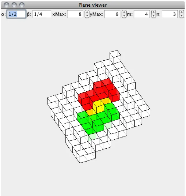
Definition 2.9. [6]((m, n)-cube, see figure 2) The (m, n)-cube wi,j(α, β, γ) at the position (i, j) of a discrete plane Pα,β,γ is the(m, n)-patternw defined by:
w(i0, j0) =pα,β,γ(i+i0, j+j0)−pα,β,γ(i, j)for all (i0, j0)∈ Fm,n
=bα(i+i0) +β(j+j0) +γc − bαi+βj+γc for all (i0, j0)∈ Fm,n
where pα,β,γ(i, j) =bαi+βj+γcandn(i, j, pα,β,γ(i, j)),
(i, j)∈Z
2odefines the discrete planeP α,β,γ.
This definition shows that:
∀(i, j)∈Z2,∀(α, β, γ)∈R3, wi,j(α, β, γ) =w0,0(α, β, αi+βj+γ).
Now, we recall some results obtained in [6], and some direct consequences of this result.
Proposition 2.10. (Recall [6])
1. The(k, l)-th point of the(m, n)-cube at the position(i, j)of the discrete planePα,β,γ can be computed by the formula :
wi,j(α, β, γ) (k, l) =
(
bαk+βlc if hαi+βj+γi< Ck,lα,β bαk+βlc+ 1 else
whereCk,lα,β= 1− hαk+βli.
2. The (m, n)-cube wi,j(α, β, γ) only depends on the interval [Bhα,β, Bhα,β+1[ containing hαi+βj+γi where theBhα,β are the numberCk,lα,β ordered by ascending order.
3. For allh∈J0, mn−1K, if[Bhα,β, Bhα,β+1[is non-empty, then there existsi, jsuch thathαi+βj+γi ∈
[Bhα,β, Bhα,β+1[. Such a way, the number of (m, n)-cubes in the discrete plane Pα,β,γ is equal to
cardnCk,lα,β
(k, l)∈ Fm,n o
≤mn.
Corollary 2.11. ([6])
1. ∀(α, β, γ)∈[0,1]2×R, w0,0(α, β, γ) =w0,0(α, β,hγi).
2. ∀(α, β, γ)∈[0,1]2×
R,∀(i, j)∈Z2,
wi,j(α, β, γ) =w0,0(α, β, αi+βj+γ)
=w0,0(α, β,hαi+βj+γi).
3. By the Proposition 2.10, the set of(m, n)-cubes of the discrete planesPα,β,γ only depends of(α, β)
and is denoted byCm,n,α,β.
Corollary 2.12. ([6]) LetObe a Farey connected component, thenOis a convex polygon and ifp1, p2, p3 are distinct vertices of the polygonO, then :
• for any pointp∈ O,
Figure 2. Example of two(4,3)-cubes (red and green)
• for any pointp∈ O in the interior of the segment of verticesp1 andp2,
Cm,n,p=Cm,n,p1∪ Cm,n,p2.
By this corollary, all the(m, n)-cubes are associated to Farey vertices. And according to the Propo-sition2.10, there are at mostmn(m, n)-cubes associated to a Farey vertex, therefore
Um,n
≤mn
3.
Fundamental properties
Lemma 3.1. (Reminder of Graph Theory) Let us consider n straight lines. The number of vertices
constructed from these nlines is at most n(n−1)
2 .
We know by [14], that the number of Farey lines, is equivalent to a polynomial of degree 3 inmand
n, when m andn go to infinity. According to Lemma3.1, these lines form a number of vertices, given at most by a polynomial of order6([6]). But this method is far from giving an optimal upper bound for the cardinality of the Farey vertices. In order to obtain a new and more powerful result of combinatorics on this set of vertices, we are going to study the properties of the Farey lines passing through a Farey vertex. Our idea is to use the theorem:
Proposition 3.2. (Reminder of Graph Theory) In a simple graph G= (V, E), we have:
X
x∈V
deg(x) = 2|E|
where V is the set of vertices, andE is the set of edges, anddeg(x)is the degree of the vertexx, that is the number of edges which are adjacent to the vertexx.
Theorem 3.3. (Gauss theorem) If(a, b, c)∈Z3, such that a|bc, anda∧b= 1. Then,a|c.
4.
Modeling of the problem of Farey vertices of order
(
m, n
)
To have a precise estimate on the number of edges in the Farey graph of order(m, n), it is sufficient to compute the degree of any Farey vertex. Henceforth, below we to study in more detail the mapping defined on F V(m, n): x7→deg(x).
Proposition 4.1. (Upper bound for the number of Farey lines of order (m, n) passing through a Farey
vertex of order(m, n)) LetP =
p
q, p0 q0
be a Farey vertex of order (m, n).
Let us define r, r0, s, s0, d andd0 as follows:
p= (p∧p0)r, q= (q∧q0)s p0= (p∧p0)r0, q0= (q∧q0)s0
d=p∧p0, d0 =q∧q0.
(1)
• If(p, p0)∈N∗2, then we have
deg(P)≤2
"
2
1
dr
mp q +n
p0
q0
+ min2jm
sr0
k
,j n s0r
k
+ 2
1
dr0
mp q +n
p0
q0
+
min2jm
sr0
k
,j n s0r
k
×2
1
d
mp q+n
p0 q0
#
.
• Ifp= 0 then we have
deg
0,p
0
q0
≤
1 +
n
q0
(2m+ 1).
The vertices such thatp= 0, are the vertices of the set
0,p
0
q0
with p
0
q0 ∈Fn
• Ifp0= 0, then we have
deg
p
q,0
≤
1 + 2
m
q
(n+ 1).
The vertices such thatp0 = 0are the vertices of the set
p q,0
with p
q ∈Fm
.
Proof. We can always suppose that in the equation of a Farey line, (of the type: uα+vβ+w = 0, with(u, v, w)∈J−m, mK×J−n, nK×Z), we have v≥0. Because ifv <0, it is sufficient to multiply the equation by−1. And we obtain the same line, but(−u,−v,−w)∈J−m, mK×J0, nK×Z.
First, we handle the case where p= 0or p0 = 0.
p= 0⇒p0v+q0w= 0⇒
(
v=q0k
w=−p0k ⇒0≤k≤ n
q0 (because of the preliminary).
There are at most 1 +
n
q0
such integers. And there are 2m+ 1integers in the interval J−m, mK. The vertices such that p= 0, are the vertices of the set
0,p
0
q0
with p
0
q0 ∈Fn
.
p0= 0⇒pu+qw= 0⇒
(
u=qk
w=−pk ⇒0≤ |k| ≤ m
q.
There are at most1 + 2
m
q
such integers. The vertices such thatp0 = 0, are the vertices of the set
p q,0
with p
q ∈Fm
.
Now, we can handle the general case remaining:
(p, p0)∈N∗2
In GF(m, n), because a Farey line generates at most 2 edges passing through the Farey vertex P, we have:
deg(P)≤2×CardnFarey Lines passing throughPo (2)
So, we are looking for an optimal bound for the cardinality of (u, v, w)∈J−m, mK×J1, nK×Zsuch
that
up q +v
p0
q0 =−w⇔
upq0+vp0q
qq0 =−w
(with the condition u∧v∧w= 1), that is
u(p∧p0)r(q∧q0)s0+v(p∧p0)r0(q∧q0)s
(p∧p0)(q∧q0)urs 0+vr0s
(q∧q0)2ss0 =−w.
After simplification:
(p∧p0)urs 0+vr0s
(q∧q0)ss0 =−w.
(p∧p0)(urs0+vr0s) =−w(q∧q0)ss0
(p∧p0)urs0=−w(q∧q0)ss0−(p∧p0)vr0s ⇒s|(p∧p0)urs0
Ass∧[(p∧p0)rs0] = 1, the Gauss theorem (Theorem3.3) implies thats|u. So,
(
∃u0∈
Zsuch thatu=su0
∃v0∈Zsuch thatv=s0v0.
So,
0≤ |u0| ≤ m
s and1≤v
0≤ n
s0.
(p∧p0)su
0rs0+s0v0r0s
(q∧q0)ss0 =−w⇒(p∧p
0)u0r+v0r0 (q∧q0) =−w
(theorem of Gauss)
⇒(p∧p0)|wand(q∧q0)|u0r+v0r0.
Whenwis fixed, the consequence of the hypothesis of primality enables to solve this diophantine equation: Let us fix w,
u0 =u0
− w
p∧p0(q∧q 0)
+r0k
v0=v0
− w
p∧p0(q∧q 0)
−rk fork∈Z
(3)
where (u0, v0)is a particular solution of the diophantine equation in(x, y): rx+r0y= 1.
The determinant of this system in
w
p∧p0, k
is:
u0q∧q0r+v0(q∧q0)r0= (q∧q0)[u0r+v0r0] =q∧q0.
So, one can determine
w p∧p0, k
by the Cramer formulas:
w p∧p0
k
!
=
− r q∧q0 −
r0
q∧q0
v0 −u0
u0 v0
.
As in [14], we can always suppose thatv≥0(else we mutiplyuα+vβ+w= 0, by−1). Moreover, we have seen that as we have:
|w| ≤mp q+n
and as p∧p0 |w, we can deduce that there existsw0 such thatw=w0(p∧p0). So,
0≤ |w0| ≤
1
p∧p0
mp q +n
p0 q0
.
As for a Farey line, (u, v)6= (0,0), we deduce that (u0, v0)6= (0,0). First we handle the case wherev= 0⇒v0= 0⇒v0
w
p∧p0
q∧q0+rk= 0⇒p|w. Asru0+r0v0= 1,
we deduce by the Bezout theorem that r∧v0 = 1. In addition to it, we have r∧(q∧q0) = 1. So, r∧(v0(q∧q0)) = 1. And by the Gauss theorem, we have that r|
w
d. In this case, it is impossible that w= 0, elsek= 0andu=v=w= 0.
So, there are at most
2
1
p
mp q+n
p0
q0
.
Farey lines passing through the Farey vertex.
In the second case, v >0, so we have
−jm s
k
≤u0 ≤jm s
k
,
1≤v0 ≤jn s0
k
.
Whenwis fixed,
r0k =u0+u0
w
p∧p0
q∧q0,
rk= v0
− w p∧p0
q∧q0−v0 fork∈Z.
So,
−jm s
k
+u0
w p∧p0
q∧q0 ≤r0k≤jm s
k
+u0
w p∧p0
q∧q0,
−jn s0
k
+v0
− w p∧p0
q∧q0 ≤rk≤ −1−v0
w
p∧p0
q∧q0 fork∈Z.
Now, we distinguish 2 cases:
• Ifw= 0, the number of suitable integers kis bounded by
min2jm
sr0
k
,j n s0r
k
.
• w6= 0
– The case wherer0k=u0
w p∧p0
q∧q0 ⇒r0|
w p∧p0
.
Then, the number of suitable w
dr0 is at most2
1
dr0
mp q +n
p0 q0
.
– Else
r0k6=u0
w
p∧p0
q∧q0,
so the number of suitable integerskis bounded by
min2jm
sr0
k
,j n s0r
and the number ofk,w d
is bounded by:
min2jm
sr0
k
,j n s0r
k
×2
1
d
mp q+n
p0
q0
.
And, of course, the existence of such couples implies that:
min2jm
sr0
k
,j n s0r
k
×2
1
d
mp q +n
p0 q0
≥1.
In particular,
jm
sr0
k
≥1
j n
s0r
k
≥1. (4)
So
CardnFarey Lines passing throughPo≤2
1
dr
mp q +n
p0 q0
+ min2jm
sr0
k
,j n s0r
k
+
2
1
dr0
mp q +n
p0 q0
+ min2jm
sr0
k
,j n s0r
k
×2
1
d
mp q +n
p0 q0
and by (2), we have
deg(P)≤2
"
2
1
dr
mp q+n
p0 q0
+ min2jm
sr0
k
,j n s0r
k
+ 2
1
dr0
mp q +n
p0 q0
+
min2jm
sr0
k
,j n s0r
k
×2
1
d
mp q+n
p0 q0
#
which proves the claim.
5.
Bound for
|
F V
(
m, n
)
|
The equations in (1) are:
r= p
p∧p0, s=
q q∧q0,
r0 = p 0
p∧p0, s 0 = q0
q∧q0,
Proposition 5.1. Let
A(m, n, p, q, p0, q0) = 2 min2jm
sr0
k
,j n s0r
k
B(m, n, p, q, p0, q0) = 4
1
dr0
mp q +n
p0 q0
C(m, n, p, q, p0, q0) = 4
1
dr
mp q+n
p0 q0
D(m, n, p, q, p0, q0) = 2
1
d
mp q +n
p0 q0
E(m, n, p, q, p0, q0) = 2A(m, n, r, r0, s, s0, d0)×D(m, n, r0, p, q, p0, q0)
A0(m, n) = X
0≤p<q≤2mn p∧q=1
X
0≤p0<q0≤2mn p0∧q0=1
A(m, n, p, q, p0, q0)
B0(m, n) = X
1≤p<q≤2mn p∧q=1
X
1≤p0<q0≤2mn p0∧q0=1
B(m, n, p, q, p0, q0)
C0(m, n) = X
1≤p<q≤2mn p∧q=1
X
1≤p0<q0≤2mn
p0∧q0=1
C(m, n, p, q, p0, q0)
D0(m, n) = X
0≤p<q≤2mn p∧q=1
X
0≤p0<q0≤2mn p0∧q0=1
D(m, n, p, q, p0, q0)
E0(m, n) = X
0≤p<q≤2mn p∧q=1
X
0≤p0<q0≤2mn p0∧q0=1
E(m, n, p, q, p0, q0)
We have:
2|F E(m, n)| ≤A0(m, n) +B0(m, n) +C0(m, n) +E0(m, n) + X p0
q0∈Fn deg
0,p
0
q0
+ X
p q∈Fm
deg
p
q,0
.
Proof. By the Proposition3.2, we have: 2|F E(m, n)| ≤P
x∈F V(m,n)deg(x)
P(α, β)∈F V(m, n)⇒ ∃
p q, p0 q0 such that
α= p
q withp∧q= 1, p≤q≤2mn β = p
0
q0 withp
0∧q0 = 1, p0 ≤q0≤2mn.
2|F E(m, n)| ≤ X 0≤p<q≤2mn
p∧q=1
X
0≤p0<q0≤2mn p0∧q0=1
deg p q, p0 q0
Lemma 5.2.
p
q, p0 q0
∈F V(m, n)⇒1≤q∨q0≤2mn.
Proof.
p
q, p0 q0
∈F V(m, n)⇒
(
∃((u, u0),(v, v0),(w, w0))∈J−m, mK 2×
J−n, nK 2×
Z2
u0v−uv06= 0
such that:
p q,
p0 q0
=
|w0v−wv0| |uv0−u0v|,
|wu0−w0u| |uv0−u0v|
.
So,q∨q0 | |uv0−u0v|.In particular,q∨q0≤2mnwhich proves the claim.
Therefore, as we remember that∀(a, b)∈N∗2,(a∧b)×(a∨b) =abwe can rewriteq∨q0=
qq0 q∧q0 =
ss0d0 ≤2mn.
We need to recall another theorem:
Theorem 5.3. [2](Asymptotic development of the harmonic series) Ifx≤1, then
X
n≤x
1
n = logx+C+O(
1
x)
where C is Euler’s constant.
We can apply this theorem and we are able to say in particular:
Corollary 5.4. There existsK >0 such that,∀n∈N\ {0,1}, we have
n
X
i=1
1
i ≤Klogn.
Proposition 5.5.
∃K >0,∀(m, n)∈N∗2, A0(m, n)≤Km2n2(m+n) ln2(mn).
Proof.
A0(m, n) = X
1≤p<q≤2mn p∧q=1
X
1≤p0<q0≤2mn p0∧q0=1
A(m, n, p, q, p0, q0)
≤ X
1≤p<q≤2mn p∧q=1
X
1≤p0<q0≤2mn p0∧q0=1
2 min2jm
sr0
k
,j n s0r
k
≤2 X
1≤p<q≤2mn p∧q=1
X
1≤p0<q0≤2mn p0∧q0=1
j n
s0r
k
≤2
2mn
X
q=1 q
X
p=0 p∧q=1
2mn
X
q0=1
q0
X
p0=1
p0∧q0=1
j n
s0r
k
I point out that I chose j n
s0r
k
, and after jm
sr0
k
, in order to obtain a symmetric upper bound. In the following, we use the boundaries forr, r0, s, s0 given by:
q=d0s so 1≤s≤ 2mn d0
q0 =d0s0 so 1≤s0≤ 2mn d0
p=dr so 1≤r≤ d
0s
d p0=dr0 so 1≤r0 ≤d
0s0
d .
Now, we can continue the calculation ofA0(m, n). For this purpose, let us permute the sums and let us change the variables by using, as before,
r = p
p∧p0, s=
q q∧q0
r0 = p 0
p∧p0, s 0 = q0
q∧q0
d =p∧p0, d0=q∧q0.
In particular,
r≤d
0s
d r0≤ d
0s0
d
⇒d≤
min
d0s
r , d0s0
r0
.
A0(m, n)≤2
2mn X q=1 q X p=0 p∧q=1
2mn
X
q0=1
q0 X
p0=1 p0∧q0=1
j n
s0r
k
≤ m+n
X
d=1 2mn
X
d0=1
b2mn d0 c
X
s=1 b2mn
d0sc
X
s0=1
d0s d
X
r=1
d0s0 d
X
r0=1 j n
s0r
k
≤ 2mn
X
d0=1
b2mn d0 c X
s=1 b2mn
d0sc
X
s0=1
d0s
X
r=1 d0s0
X
r0=1 j n
s0r
k
j min(d0s
r ,d
0s0
r0 )
k
X
d=1
1.
Now, we have to distinguish the case whered0s= 1and the cased0s >1 in the sums in order to use the Corollary5.4 (and the same ford0s0).
A0≤ 2mn
X
d0=1
b2mn d0 c
X
s=1 b2mn
d0sc
X
s0=1
d0s
X
r=1 d0s>1
d0s0
X
r0=1 d0s0>1
d0 n
rr0 +Km
2n3ln2
(mn)
≤K0nln2(mn)
2mn
X
d0=1
d0 b2mn
d0 c
X
s=1 b2mn
d0sc
X
s0=1
1 +Km2n3ln2(mn)
≤K0nln2(mn)
2mn
X
d0=1
d0 b2mn
d0 c
X
s=1
2mn d0s +Km
≤K0nln2(mn)
2mn
X
d0=1
b2mn d0 c
X
s=1
2mn
s +Km
2n3ln2(mn)
≤K0nln2(mn)
2mn
X
s=1 b2mn
s c
X
d0=1
2mn
s +Km
2n3ln2
(mn)
≤K0m2n3ln2(mn)
2mn
X
s=1
1
s2 +Km 2n3ln2
(mn)
≤K”m2n3ln2(mn)
A0(m, n) = X
1≤p<q≤2mn p∧q=1
X
1≤p0<q0≤2mn p0∧q0=1
A(p, q, p0, q0)
≤ X
1≤p<q≤2mn p∧q=1
X
1≤p0<q0≤2mn
p0∧q0=1
4jm
sr0
k
≤4 X
1≤p<q≤2mn p∧q=1
X
1≤p0<q0≤2mn p0∧q0=1
jm sr0 k ≤4 2mn X q=1 q X p=1 p∧q=1
2mn
X
q0=1
q0
X
p0=1
p0∧q0=1
jm
sr0
k
≤ m+n
X
d=1 2mn
X
d0=1
b2mn d0 c X
s=1 b2mn
d0sc
X
s0=1
d0s d
X
r=1
d0s0 d
X
r0=1 jm sr0 k ≤ 2mn X
d0=1
b2mn d0 c X
s=1 b2mn
d0sc
X
s0=1
d0s
X
r=1 d0s0
X
r0=1 jm
sr0
k
j min(d0s
r , d0s0
r0 )
k X d=1 1 ≤ 2mn X
d0=1
b2mn d0 c
X
s=1 b2mn
d0sc
X
s0=1
d0s
X
r=1 d0s0
X
r0=1
m sr0
d0s r
≤ 2mn
X
d0=1
b2mn d0 c
X
s=1 b2mn
d0sc
X
s0=1
d0s
X
r=1 d0s>1
d0s0
X
r0=1 d0s0>1
d0m rr0 +Kn
2m3ln2(mn)
≤K0mln2(mn)
2mn
X
d0=1
d0 b2mn
d0 c X
s=1 b2mn
d0sc
X
s0=1
1 +Kn2m3ln2(mn)
≤K0mln2(mn)
2mn
X
d0=1
b2mn d0 c
X
s=1
2mn d0s +Kn
2m3ln2(mn)
≤K0m2nln2(mn)
2mn
X
d0=1
b2mn d0 c
X
s=1
1
s+Kn
≤K”n2m3ln2(mn).
Proposition 5.6.
∃K >0,∀(m, n)∈N∗2, B0(m, n)≤Km2n2(m+n) ln2(mn).
Proof.
B0(m, n) = X
1≤p<q≤2mn p∧q=1
X
1≤p0<q0≤2mn p0∧q0=1
B(p, q, p0, q0)
≤ X
1≤p<q≤2mn p∧q=1
X
1≤p0<q0≤2mn p0∧q0=1
4
1
dr0
mp q +n
p0
q0
≤K[B01(m, n) +B20(m, n)]
where
B10(m, n) =m X 1≤p<q≤2mn
p∧q=1
X
1≤p0<q0≤2mn
p0∧q0=1 r r0sd0
B20(m, n) =n X 1≤p<q≤2mn
p∧q=1
X
1≤p0<q0≤2mn p0∧q0=1
1
d0s0
B01(m, n)≤m 2mn
X
q=1 q
X
p=1 p∧q=1
2mn
X
q0=1
q0
X
p0=1 p0∧q0=1
r r0sd0
≤m 2mn
X
d0=1
b2mn d0 c
X
s=1 b2mn
d0sc
X
s0=1
d0s
X
r=1 d0s0
X
r0=1
j min(d0s
r ,d
0s0
r0 )
k
X
d=1
r r0sd0
≤m 2mn
X
d0=1
b2mn d0 c X
s=1 b2mn
d0sc
X
s0=1
d0s
X
r=1 d0s0
X
r0=1
1
r0
Now, we have to distinguish the case whered0s0 = 1and the cased0s0>1in the sum in order to use the Corollary5.4.
B10(m, n)≤K0m 2mn
X
d0=1
b2mn d0 c
X
s=1 b2mn
d0sc
X
s0=1
d0sln(d0s0) +Km3n2ln2(mn)
≤K0mln(2mn)
2mn
X
d0=1
b2mn d0 c
X
s=1
d0s2mn d0s +Km
≤K0m2nln(2mn)
2mn
X
d0=1
b2mn d0 c X
s=1
1 +Km3n2ln2(mn)
≤K0m2nln(2mn)
2mn
X
d0=1
2mn d0 +Km
3n2ln2(mn)
≤K”m3n2ln2(mn).
B20(m, n)≤n 2mn
X
q=1 q
X
p=1 p∧q=1
2mn
X
q0=1
q0
X
p0=1 p0∧q0=1
1
d0s0
≤n 2mn
X
d0=1
b2mn d0 c
X
s=1 b2mn
d0sc
X
s0=1
d0s
X
r=1 d0s0
X
r0=1
j min(d0s
r , d0s0
r0 ) k
X
d=1
1
d0s0
≤n 2mn
X
d0=1
b2mn d0 c
X
s=1 b2mn
d0sc
X
s0=1
d0s
X
r=1 d0s0
X
r0=1
1
r0
≤K0n 2mn
X
d0=1
b2mn d0 c X
s=1 b2mn
d0sc
X
s0=1
d0sln(d0s0) +Kn3m2ln2(mn)
≤K0nln(2mn)
2mn
X
d0=1
b2mn d0 c
X
s=1
d0s2mn d0s +Kn
3m2ln2(mn)
≤K0n2mln(2mn)
2mn
X
d0=1
b2mn d0 c
X
s=1
1 +Kn3m2ln2(mn)
≤K0n2mln(2mn)
2mn
X
d0=1
2mn d0 +Kn
3m2ln2
(mn)
≤K”n3m2ln2(mn).
Proposition 5.7.
∃K >0,∀(m, n)∈N∗2, C0(m, n)≤Km2n2(m+n) ln2(mn).
Proof.
C0(m, n) = X
1≤p<q≤2mn p∧q=1
X
1≤p0<q0≤2mn p0∧q0=1
C(p, q, p0, q0)
≤ X
1≤p<q≤2mn p∧q=1
X
1≤p0<q0≤2mn p0∧q0=1
4
1
dr
mp q +n
p0 q0
where
C10(m, n) =m X 1≤p<q≤2mn
p∧q=1
X
1≤p0<q0≤2mn p0∧q0=1
1
sd0
C20(m, n) =n
X
1≤p<q≤2mn p∧q=1
X
1≤p0<q0≤2mn p0∧q0=1
r0
rd0s0.
C10(m, n)≤m 2mn X q=1 q X p=1 p∧q=1
2mn
X
q0=1
q0
X
p0=1 p0∧q0=1
1
sd0
≤m 2mn
X
d0=1
b2mn d0 c
X
s=1 b2mn
d0sc
X
s0=1
d0s
X
r=1 d0s0
X
r0=1
j min(d0s
r , d0s0
r0 ) k X d=1 1 sd0 ≤m 2mn X
d0=1
b2mn d0 c
X
s=1 b2mn
d0sc
X
s0=1
d0s
X
r=1 d0s0
X
r0=1
1
r
≤K0m 2mn
X
d0=1
b2mn d0 c X
s=1 b2mn
d0sc
X
s0=1
d0s0ln(d0s) +Km3n2ln2(mn)
≤K0mln(2mn)
2mn
X
d0=1
b2mn d0 c
X
s0=1
d0s02mn d0s0 +Km
3n2ln2
(mn)
≤K0m2nln(2mn)
2mn
X
d0=1
b2mn d0 c
X
s0=1
1 +Km3n2ln2(mn)
≤K0m2nln(2mn)
2mn
X
d0=1
2mn d0 +Km
3n2ln2
(mn)
≤K”m3n2ln2(mn).
C20(m, n)≤n 2mn X q=1 q X p=1 p∧q=1
2mn
X
q0=1
q0
X
p0=1 p0∧q0=1
r0 rd0s0
≤n 2mn
X
d0=1
b2mn d0 c X
s=1 b2mn
d0sc
X
s0=1
d0s
X
r=1 d0s0
X
r0=1
j min(d0s
r , d0s0
r0 )
k
X
d=1
r0 rd0s0
≤n 2mn
X
d0=1
b2mn d0 c
X
s=1 b2mn
d0sc
X
s0=1
d0s
X
r=1 d0s0
X
r0=1
r0 rd0s0
≤K0n 2mn
X
d0=1
b2mn d0 c X
s=1 b2mn
d0sc
X
s0=1
d0s0ln(d0s) +Kn3m2ln2(mn)
≤K0nln(2mn)
2mn
X
d0=1
b2mn d0 c
X
s0=1
d0s02mn d0s0 +Kn
3m2ln2
(mn)
≤K0n2mln(2mn)
2mn
X
d0=1
b2mn d0 c
X
s0=1
1 +Kn3m2ln2(mn)
≤K0n2mln(2mn)
2mn
X
d0=1
2mn d0 +Kn
3m2ln2
(mn)
≤K”n3m2ln2(mn).
Proposition 5.8.
∃K >0, ∀(m, n)∈N∗2, E0(m, n)≤Km2n2(m+n) ln(mn).
Proof.
E0(m, n) = X
1≤p<q≤2mn p∧q=1
X
1≤p0<q0≤2mn p0∧q0=1
E(p, q, p0, q0)
≤ X
1≤p<q≤2mn p∧q=1
X
1≤p0<q0≤2mn p0∧q0=1
2A(m, n, r, r0, s, s0, d0)×D(m, n, r0, p, q, p0, q0)
≤K X
1≤p<q≤2mn p∧q=1
X
1≤p0<q0≤2mn p0∧q0=1
min2jm
sr0
k
,j n s0r
k1
d
mp q +n
p0 q0
≤K[E10(m, n) +E02(m, n)]
with the condition (4).
E10(m, n) =mn X 1≤p<q≤2mn
p∧q=1
X
1≤p0<q0≤2mn
p0∧q0=1
1
s0r 1
d p q.
E20(m, n) =mn X 1≤p<q≤2mn
p∧q=1
X
1≤p0<q0≤2mn p0∧q0=1
1
sr0 1
d p0 q0.
Let us study further E10(m, n), then the results forE
0
2(m, n)are computed in a similar manner.
E10(m, n)≤mn X 1≤p<q≤2mn
p∧q=1
X
1≤p0<q0≤2mn
p0∧q0=1
1
s0 1
q
≤mn X
1≤p<q≤2mn p∧q=1
X
1≤p0<q0≤2mn p0∧q0=1
1
≤mn 2mn
X
d0=1
b2mn d0 c X
s=1 b2mn
d0sc
X
s0=1
d0s
X
r=1 bn
s0rc≥1 d0s0
X
r0=1 bm
sr0c≥1
j min(d0s
r ,d
0s0
r0 )
k
X
d=1
1
ss0d0
≤mn 2mn
X
d0=1
b2mn d0 c X
s=1 b2mn
d0sc
X
s0=1
d0s
X
r=1 bn
s0rc≥1 d0s0
X
r0=1 bm
sr0c≥1
d0s0 r0
1
ss0d0
≤mn 2mn
X
d0=1
b2mn d0 c X
s=1 b2mn
d0sc
X
s0=1
d0s
X
r=1 bn
s0rc≥1 d0s0
X
r0=1
bm sr0c≥1 d0s0>1
1
r0s+Km
2n3ln(mn)
≤K0mn2ln(mn)
2mn
X
d0=1
b2mn d0 c X
s=1 b2mn
d0sc
X
s0=1
1
ss0 +Km
2n3ln(mn)
≤K0m2n3ln(mn)
b2mn d0 c
X
s=1 b2mn
d0sc
X
s0=1
1
s2s02 +Km
2n3ln(mn)
≤K”m2n3ln(mn).
The computation is exactly the same for E20(m, n).
It remains to treat the two simple cases wherep= 0orp0= 0 of the Proposition4.1:
Proposition 5.9.
∃K >0,∀(m, n)∈N∗2, X
p0 q0∈Fn
deg
0,p
0
q0
+ X
p q∈Fm
deg
p
q,0
≤Kmn(m2+n2).
Proof. • 1 + n q0
(2m+ 1)
≤2m+ 1 + 2nm+n≤5mn+ 1
X
p0 q0∈Fn
deg
0,p
0
q0
≤ X
p0 q0∈Fn
1 + n q0
(2m+ 1)
≤ X
p0 q0∈Fn
(5mn+ 1)≤(5mn+ 1)|Fn|
•
1 + 2
m
q
(n+ 1)
≤n+ 1 + 2mn+ 2m≤5mn+ 1
X
p q∈Fm
deg
p
q,0
≤ X
p q∈Fm
1 + 2
m
q
(n+ 1)
≤ X
p q∈Fm
(5mn+ 1)≤(5mn+ 1)|Fm|
We know [29] that
|Fn|= 1 +
n
X
k=1
ϕ(k) ∼ +∞
n2
So there exists K >0 such that
X
p0 q0∈Fn
deg
0,p
0
q0
+ X
p q∈Fm
deg
p
q,0
≤Kmn(m2+n2).
Hence, we have:
∃K >0,∀(m, n)∈N∗2, 2|F E(m, n)|= X
x∈F V(m,n)
deg(x)≤Km2n2(m+n) ln2(mn).
So, we can say that:
∃K≥0, |F E(m, n)| ≤Km2n2(m+n) ln2(mn).
Hence, in the Farey graph of order(m, n), we have:
Proposition 5.10.
∃K >0,∀(m, n)∈N∗2, |F E(m, n)| ≤Km2n2(m+n) ln2(mn).
Moreover, as the Farey graph of order(m, n)is planar, we can apply to it the Euler’s Formula:
Theorem 5.11. (Recall)(Euler’s formula for the connex planar graphs) In a connex planar multi-graph, having V vertices, E edges, and F facets, we have: V −E+F = 2.
In particular, this involves that we haveV ≤E+ 2.
∃K >0,∀(m, n)∈N∗2, |F V(m, n)| ≤Km2n2(m+n) ln2(mn).
This greatly improves the upper bound previously found in [6]. And we can add:
∃K >0,∀(m, n)∈N∗2, |F F(m, n)| ≤Km2n2(m+n) ln2(mn).
Corollary 5.12. (Upper bound for the(m, n)-cubes)
∃K >0,∀(m, n)∈N∗2, |Umn| ≤Km3n3(m+n) ln2(mn).
6.
Summary-conclusion
In order to improve the upper bound for
Um,n
, an interesting work using combinatorics, graph
theory, and number theory, has been to focus on the diophantine aspects of Farey diagrams, combined with some other arguments of graph theory to estimate better the cardinality of Farey vertices. And in this work, we obtained two important results:
•
∃C >0,∀(m, n)∈N∗2,
F V(m, n) ≤Cm
2n2(m+n) ln2
(mn)
• And we obtained:
∃C >0,∀(m, n)∈N∗2, Um,n
≤Cm
3n3(m+n) ln2
(mn)
whereas the previous published result existing was a polynomial of degree 8 [6].
Acknowledgment: I dedicate this work to the memory of my beloved father, who did his best for me and for the science. I also want to thank my brother(and his wife) and my sister(and her husband) for their support during the preparation of this article. I am thankful to Grégory Apou for his help. I also would like to thank the Professor Andre Leroy for his meaningful help, his expertise in algebra, and for having given to me an invitation to give a successful seminar on Combinatorics and Number Theory, and their applications to Computer Sciences, in the L.M.L. of the University of Artois, on January, 2015. I also thank the director of the I.M.B., the Professor Alain Bachelot for his help, and two other persons: Professor Hugues Talbot, and Professor Pierre Villon for their great kindness. And I also thank the experts of Number Theory: Henri Cohen and Yuri Bilu for their advises. My gratitude also goes to David, and Jacques(and his wife) the friends of my father, for their encouragement to publish this article. This work could not take his final version without the meaningful help of the anonymous referees to whom I express my sincere acknowledgements for their insightful remarks, as they carefully reviewed my work and gave generously of their time and their expertise.
References
[1] D. M. Acketa and J. D. Žunić,On the number of linear partitions of the (m, n)-grid, Inform. Process. Lett., 38(3), 163-168, 1991.
[2] T. M. Apostol,Introduction to Analytic Number Theory, Springer-Verlag, 1976.
[3] T. Asano and N. Katoh, Variants for the hough transform for line detection, Comput. Geom., 6(4), 231-252, 1996.
[4] J. M. Chassery, D. Coeurjolly and I. Sivignon, Duality and geometry straightness, characterization and envelope, Discrete Geometry for Computer Imagery, Springer, 1-16, 2006.
[5] J. M. Chassery and A. Montanvert, Geometrical representation of shapes and objects for visual perception, Geometric Reasoning for Perception and Action, Springer, 163-182, 1993.
[6] A. Daurat, M. Tajine and M. Zouaoui, About the frequencies of some patterns in digital planes application to area estimators, Comput. Graph., 33(1), 11-20, 2009.
[7] I. Debled-Rennesson,Etude et reconnaissance des droites et plans discrets, PhD thesis, 1995. [8] E. Domenjoud, D. Jamet, D. Vergnaud and L. Vuillon, Enumeration formula for (2, n)-cubes in
discrete planes, Discrete Appl. Math., 160(15), 2158-2171, 2012.
[9] E. Szemerédi and W. T. Trotter Jr.,Extremal problems in discrete geometry, Combinatorica, 3(3-4), 381-392, 1983.
[10] A. Hatcher, Topology of numbers, Unpublished manuscript, in preparation; see http://www.math.cornell.edu/~hatcher/TN/TNpage.html.
[11] P. Haukkanen and J. K. Merikoski, Asymptotics of the number of threshold functions on a two-dimensional rectangular grid, Discrete Appl. Math., 161(1), 13-18, 2013.
[12] W. Hou and C. Zhang, Parallel-beam ct reconstruction based on mojette transform and compressed sensing, International Journal of Computer and Electrical Engineering, 5(1), 83-87, 2013.
[13] Y. Kenmochi, L. Buzer, A. Sugimoto and I. Shimizu,Digital planar surface segmentation using local geometric patterns, Discrete Geometry for Computer Imagery, Springer, 322-333, 2008.
[14] D. Khoshnoudirad,Farey lines defining Farey diagrams, and application to some discrete structures, Appl. Anal. Discrete Math., 9(1), 73-84, 2015.
[15] A. O. Matveev,A note on Boolean lattices and Farey sequences, Integers, 7, A20, 2007.
[17] A. O. Matveev,Neighboring fractions in Farey subsequences, arXiv:0801.1981, 2008. [18] A. O. Matveev,A note on Boolean lattices and Farey sequences II, Integers, 8, A24, 2008.
[19] M. D. McIlroy,A note on discrete representation of lines, AT&T Technical Journal, 64(2), 481-490, 1985.
[20] E. Remy and E. Thiel, Exact medial axis with euclidean distance, Image and Vision Computing, 23(2), 167-175, 2005.
[21] E. Remy and E. Thiel,Structures dans les spheres de chanfrein, RFIA, 483-492, 2000.
[22] I. Svalbe and A. Kingston, On correcting the unevenness of angle distributions arising from integer ratios lying in restricted portions of the Farey plane, Combinatorial Image Analysis, Springer, 110-121, 2005.
[23] G. Tenenbaum, Introduction to analytic and probabilistic number theory, 46, Cambridge University Press, 1995.
[24] E. Thiel, Les distances de chenfrein en analyse d’images : fondements et applications, Thélse de doctorat, UJF Grenoble, 1994.
[25] E. Thiel and A. Montanvert, Chamfer masks: Discrete distance functions, geometrical properties and optimization, Pattern Recognition, Vol. III. Conference C: Image, Speech and Signal Analysis, Proceedings., 11th IAPR International Conference on, IEEE, 244-247, 1992.
[26] R. Tomás,Asymptotic behavior of a series of Euler’s totient functionϕ(k)times the index of1/k in a Farey sequence, arXiv:1406.6991, 2014.
[27] R. Tomás,From farey sequences to resonance diagrams, Physical Review Special Topics-Accelerators and Beams, 17(1), 014001, 2014.
[28] V. Trifonov, L. Pasqualucci, R. Dalla-Favera and R. Rabadan, Fractal-like distributions over the rational numbers in high-throughput biological and clinical data, Scientific reports, 1, 2011.