STATISTICAL METHODS
FOR COMPETING RISKS IN CASE-COHORT STUDIES
Adane Fekadu Wogu
A dissertation submitted to the faculty at the University of North Carolina at Chapel Hill in partial fulfillment of the requirements for the degree of Doctor of Philosophy in the Department of
Biostatistics in the Gillings School of Global Public Health.
Chapel Hill 2020
Approved by: Jianwen Cai Hazel B. Nichols Chirayath Suchindran Donglin Zeng
c
2020
ABSTRACT
Adane Fekadu Wogu: Statistical Methods for Competing Risks in Case-Cohort Studies
(Under the direction of Jianwen Cai)
The case-cohort study design is a cost-effective study design for large-scale follow-up studies, especially when the events are rare. Large-scale follow-up studies are also subject to competing risks – a situation where there are multiple causes of failure and the occurrence of one type of event prohibits the occurrence of the other types of events. There are two families of regression models in studying time to event data with competing risks: modeling for the cause-specific hazard or modeling the subdistribution (also called cumulative incidence function) of a competing risk. In this dissertation, we consider modeling the subdistribution of competing risk in case-cohort studies. We consider semiparametric proportional subdistribution hazards (PSH) and additive subdistribution hazards (ASH) models for an event of interest in the presence of competing risks in case-cohort studies. We propose estimating equations for each of the two models utilizing inverse probability weighting (IPW) techniques for the estimation of regression parameters. For both proposed methods of PSH and ASH models, the resulting estimators from their respective estimating equations are shown to be consistent and asymptotically normal under some regularity conditions. Further, simulation studies are carried out for both methods to examine the finite sample properties of the estimators. For illustration, the proposed methods are applied to case-cohort data from the Sister Study (Sandler et al. 2017).
ACKNOWLEDGEMENTS
I would like to express my deepest gratitude to my dissertation advisor, Dr. Jianwen Cai, for her invaluable guidance, encouragement and tremendous assistance throughout my dissertation research. I feel fortunate to have worked with her on my dissertation; and she has set an example of excellence as an advisor, researcher, instructor, and role model. I am also very thankful for her financial support.
I am greatly indebted to Dr. Chirayath Suchindran, my academic advisor, for his unwavering support and guidance. I would also like to thank my committee members, Drs. Hazel Nichols, Donglin Zeng, and Shanshan Zhao, whose constructive feedback and suggestions have strengthened this dissertation immeasurably. I would especially like to thank Dr. Shanshan Zhao for her remarkable comments on this dissertation as well as helping me get the Sister Study data from the National Institute of Environmental Health Sciences (NIEHS). My gratitude also goes to NIEHS and Dr. Dale Sandler for providing the Sister Study data. I am sincerely thankful to Veronica Stallings and Melissa Hobgood, who always had my back and helped me overcome difficulties during my study. I am extremely thankful for your support through the ups and downs of my academic career. My words would become inadequate if I were to miss acknowledging the Department of Biostatistics and my professors. Without their help, I would not have been able to achieve this degree.
I am especially grateful to my loving wife, Masti, for being my inspiration through what has been arduous years of doctoral study. I cannot thank you enough for your love, patience and emotional support. I must also thank my son, Ethan, who has never considered his dad anything but student, I suppose. To my parents and siblings, thank you for your unconditional trust, continuous encouragement, and limitless patience. There are not enough words to describe how thankful I am to all of you. To my friends, thank you for encouraging me in all of my pursuits and inspiring me to follow my dreams.
TABLE OF CONTENTS
LIST OF TABLES . . . . viii
LIST OF FIGURES . . . . ix
CHAPTER 1: INTRODUCTION . . . . 1
CHAPTER 2: LITERATURE REVIEW . . . . 5
2.1 Case-Cohort Study Design . . . 5
2.2 The Proportional Hazards Model . . . 7
2.2.1 Proportional hazards model for cohort studies . . . 8
2.2.2 Proportional hazards model for case-cohort studies . . . 10
2.3 Additive Hazards Model for Case-Cohort Studies . . . 21
2.4 Statistical Approaches for Competing Risks . . . 25
2.4.1 Latent failure times approach . . . 25
2.4.2 Cause-specific hazards approach . . . 26
2.4.3 Subdistribution hazards approach . . . 28
2.4.4 Cause-specific hazards model versus subdistribution hazards model . . . 29
2.4.5 Proportional hazards model for the subdistribution of a competing risk . . . 30
2.4.6 Competing risk analysis in case-cohort studies . . . 32
2.5 Testing the Proportional Hazards Assumption . . . 36
2.5.1 Assessing the proportional hazards assumption using the partial and weighted residuals . . . 37
2.5.2 Regression approach to assess nonproportionality . . . 38
CHAPTER 3: PROPORTIONAL SUBDISTRIBUTION HAZARDS MODEL FOR COMPETING RISKS IN CASE-COHORT STUDIES . . . . 42
3.1 Introduction . . . 42
3.2 Data Structure and Model . . . 44
3.2.1 Data structure with competing risks . . . 44
3.2.2 Case-cohort sampling design in the presence of competing risks . . . 45
3.2.3 The proportional subdistribution hazards model . . . 45
3.4 Asymptotic Properties . . . 47
3.5 Simulation Studies . . . 52
3.6 Application to the Sister Study . . . 54
3.7 Concluding Remarks . . . 56
3.8 Proofs of Theorems . . . 57
CHAPTER 4: ADDITIVE SUBDISTRIBUTION HAZARDS REGRESSION FOR COMPETING RISKS DATA IN CASE-COHORT STUDIES . . . . 83
4.1 Introduction . . . 83
4.2 Data Structure and Model . . . 85
4.2.1 Data structure with competing risks . . . 85
4.2.2 Case-cohort sampling design in the presence of competing risks . . . 86
4.2.3 The additive subdistribution hazards model . . . 87
4.3 Estimation . . . 87
4.4 Asymptotic Properties . . . 90
4.5 Simulation Studies . . . 93
4.6 Application to Sister Study . . . 95
4.7 Concluding Remarks . . . 98
4.8 Proofs of Theorems . . . 99
CHAPTER 5: ASSESSING THE PROPORTIONAL HAZARDS ASSUMP-TION OF FINE-GRAY MODEL IN CASE-COHORT STUDIES . . . . 117
5.1 Introduction . . . 117
5.2 Methods . . . 119
5.2.1 Data structure . . . 119
5.2.2 Correlation test based on Schoenfeld-type residuals . . . 120
5.2.3 Regression approach for nonpropotionality tests: Score test . . . 122
5.3 Simulation Studies . . . 123
5.4 Application to the Sister Study . . . 126
5.5 Concluding Remarks . . . 128
5.6 Supplementary Materials . . . 128
CHAPTER 6: SUMMARY AND FUTURE CONSIDERATIONS . . . . 139
LIST OF TABLES
3.1 Summary of simulation results for ( ˆβ11,βˆ12) when (β11, β12) = (0.5,0.5),
Z1 ∼N(0,1), Z2 ∼N(0,1),p= 0.3,and n= 4,000 . . . 79 3.2 Summary of simulation results for ( ˆβ11,βˆ12) when (β11, β12) = (1.0,0.5),
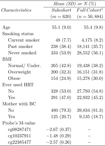
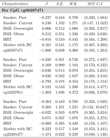
Z1 ∼Bin(0.5),Z2 ∼N(0,1),p= 0.5,and n= 4,000 . . . 80 3.3 Baseline characteristics of Sister Study (the subcohort and the full cohort) . . . 81 3.4 Estimated coefficients and standard errors in models for invasive breast
cancer in the Sister Study . . . 82 4.1 Summary of simulation results for ( ˆβ11,βˆ12) when (β11, β11) = (0.5,0.5),
Z1 ∼U(0,1), Z2 ∼U(1,2),p= 0.4,and n= 4,000 . . . 114 4.2 Summary of simulation results for ( ˆβ11,βˆ12) when (β11, β11) = (1.0,0.5),
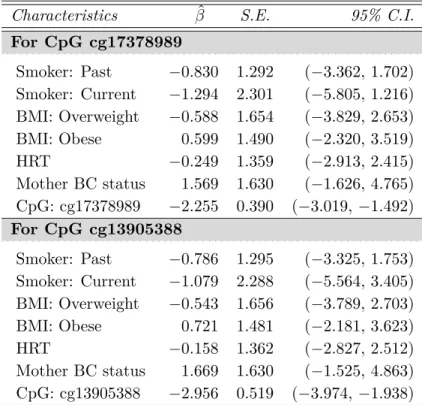
Z1 ∼Bin(0.5),Z2 ∼U(1,2),p= 0.4,and n= 4,000 . . . 115 4.3 Analysis of Sister Study; CpGs: cg17378989 (ERCC1 gene) and
cg13905388 (CDCA4 gene) . . . 116 5.1 Subcohort sizes (approximate) of the case-cohort sampled from the full
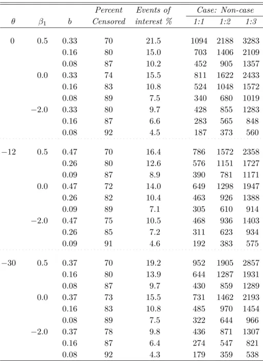
cohorts (N = 4,000) for the PSH models under the three scenarios: (i)β(t) =β1 (i.e., θ= 0), (ii)β(t) =β1+θtwith θ=−12,and (iii)β(t)
=β1+θt2 withθ=−30.In all scenarios,γ = 1.4 and ϕ=−3.5.
Censo-ring times were generated fromU nif[0.05, b]. . . 132 5.2 Empirical Type I errors from the proposed methods to assess
nonpropo-rtionality by testingH0:θ= 0 for PSH models under the scenario: β(t)
=β1 (i.e.,θ= 0). We setγ = 1.4 and ϕ=−3.5.. . . 133 5.3 Empirical Type I errors from the proposed methods to assess
nonpropo-rtionality by testingH0:θ= 0 for PSH models under the two scenarios: (i)β(t) =β1+θtwith θ=−12,and (ii)β(t) =β1+θt2 withθ=−30.
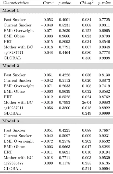
We set γ = 1.4 andϕ=−3.5 in both scenarios. . . 134 5.4 Tests of the proportionality assumption in three PSH models for invasive
breast cancer in the Sister Study (case-cohort data) based on two
LIST OF FIGURES
5.1 Plots of Schoenfeld-type residuals in PSH models for invasive breast
can-cer in the Sister Study (CpG: cg08287471/ NEK6) . . . 136 5.2 Plots of Schoenfeld-type residuals in PSH models for invasive breast
can-cer in the Sister Study (CpG: cg10237911/ANKRA2) . . . 137 5.3 Plots of Schoenfeld-type residuals in PSH models for invasive breast
CHAPTER 1: INTRODUCTION
Epidemiologic cohort studies and disease prevention trials typically require the follow-up of several thousand subjects for a number of years before yielding useful results, and hence can be prohibitively expensive (Prentice, 1986). Such studies involving costly or time-consuming methods to obtain covariate information, such as interviews, use of precious biological specimens, collecting hospital or employment records, or genotyping, can be carried out more efficiently by oversampling cases because cases contain more information on disease risk, especially when the event rate is low (Breslow and Day, 1987; Barlow, 1994; Cologne et al., 2012). For prospective studies with rare diseases, Prentice (1986) proposed the adequate and cost effective study design, known as the case-cohort study design.
function) for which estimation and inference procedures can be carried out by implementing the partial likelihood principle and weighting techniques.
In this dissertation, we propose statistical techniques for the proportional as well as additive subdistribution hazards models in the presence of competing risks in case-cohort study designs. Proportional Subdistribution Hazards Models in the Presence of Competing Risks in Case-Cohort Studies
A case-cohort study design involves the collection of covariate information for all failures in the entire cohort and a random sample of the cohort, or “subcohort” which is designated prospectively as the source of comparison observations for the observed failures (Prentice, 1986; Barlow et al., 1999). Prentice (1986) presented the application of proportional hazards regression model for case-cohort studies and, through pseudolikelihood approach which mimics the form of partial likelihood, proposed an estimating equation for the estimation of regression parameters. A variance estimator, which requires computation of covariances among score components arising from the sampling design, was also proposed. Self and Prentice (1988), with a slight modification of the pseudolikelihood function, subsequently provided a revised variance estimator and justified the asymptotic normality of the estimator under mild regularity conditions. Following Prentice (1986) and Self and Prentice’s (1988) breakthrough of the analysis of data from case-cohort study designs, proportional hazard models for such study designs when there is a single, possibly censored failure time on each subject have been extensively studied in literature (Barlow, 1994; Therneau and Li, 1999; Borgan et al., 2000; Chen, 2001; Kalbfleisch and Prentice, 2002; Kong and Cai, 2009; Kim et al., 2013).
In time-to-event data analysis in cohort studies, the original cohort may have such important aspect that the failure on a subject may be one of several distinct failure types. That is, each subject may fail one of theK (K ≥2) causes, called competing risks (competing causes of failure). Considering the broad use of the cumulative incidence function (also known as the subdistribution and the marginal probability function) especially in predictive models, Fine and Gray (1999) proposed a semiparametric approach to directly model the subdistribution of an event of interest under the proportional hazards formulation and derived estimation as well as inference procedures for the regression parameters using the partial likelihood principle and weighting techniques.
primarily favored statistical approach (compared to the additive hazards model) for time-to-event data with explanatory covariates, the first part of this dissertation aims at developing statistical approaches for the proportional subdistribution hazards model in case-cohort studies in presence of competing risks. The proposed methods will be assessed in numerical studies through simulations followed by the analysis of a dataset from the Sister Study of the Environmental and Genetic Risk Factors for Breast Cancer, a nationwide study conducted by the National Institute of Environmental Health Sciences (NIEHS).
Additive Subdistribution Hazards Models in the Presence of Competing Risks in Case-Cohort Studies
In Cox proportional hazard regression models, the hazard function is assumed to be related to the covariates multiplicatively in such a way that the model quantifies the joint effects of exposures on the relative risk of disease. This model is popular and has been the first method of choice for time-to-event data because it is intuitive, possess straightforward application of the partial likelihood approach, its results have simple interpretation and statistical software packages are largely available for analysis (Lin and Ying, 1994). While the role of multiplicative models, such as the Cox proportional hazards models, is unequivocal, there are a number of situations in epidemiology or disease prevention studies in which addressing the absolute difference in hazards or the change in hazard function due to the exposure is of the main interest.
A well-recognized but less often used method for analyzing time-to-event data which considers the absolute difference in hazards is an additive hazards regression model. The additive hazards regression model linearly relates the conditional hazard function of the failure time to the covariates. Lin and Ying (1994) proposed a semiparametric approach for additive hazards model which possesses simple procedures with high efficiencies for making inference about the regression parameters. The proposed techniques resemble those of the proportional hazards model as they characterize the martingale feature of the partial likelihood score function used in Cox proportional hazards model (Cox, 1972). Kulich and Lin (2000a) demonstrated the use of case-cohort data to estimate the regression parameters of the additive hazards model and the estimator is shown to be consistent and asymptotically normal with an easily estimated variance.
models for the cumulative incidence function in the presence of competing risks in case-cohort study designs. In the second part of this dissertation, we propose statistical methods for additive subdistribution hazards model in the presence of competing risks in case-cohort study designs. The proposed methods will be assessed through data simulations and the analysis of a dataset from the Sister Study.
Goodness-of-Fit Assessment in Proportional Subdistribution Hazards Models in the Presence of Competing Risks in Case-Cohort Studies
The enormous success and extensive utilization of the Cox proportional hazards model have made a way to the importance of model checking, especially testing the proportional hazards assumption. In literature, a number of procedures have been proposed to check and verify the proportional hazards assumption in full cohort studies (Schoenfeld, 1982; Andersen, 1982; Gray, 1990; Lin et al., 1993; Grambsch and Therneau; 1994). Further, Zhou et al. (2013) proposed a goodness-of-fit test for proportional subdistribution hazards model in cohort studies, specifically to test the proportionality assumption of the proportional subdistribution hazards model in the presence of competing risks (i.e., the Fine-Gray model). Aside from cohort studies, Xue et al. (2013) established a method to assess proportional hazards assumption in case-cohort studies by extending the approach used for similar assessment in standard Cox proportional hazards model. Noting the importance of checking the assumption, we propose two approaches to assess the proportionality assumption in the proportional subdistribution hazards model in presence of competing risks in case-cohort study designs, for which we proposed parameter estimation and inference procedures. The proposed assessment methods will be investigated using simulation studies as well as by applying them on a dataset from the Sister Study.
CHAPTER 2:LITERATURE REVIEW
2.1 Case-Cohort Study Design
A case-cohort study design was first introduced by Ross L. Prentice in 1986 in order to reduce the cost of large cohort studies when there is only one event of interest, the failure rate is considerably low (e.g. rare disease) and some exposures are expensive to measure. The case-cohort design involves the selection of a random sample, or a stratified random sample, of the entire cohort, called subcohort, and collection of covariate information only for the sampled random subcohort and for all cases (Prentice, 1986). Note that: (1) the cases in the entire cohort are included in the case-cohort design with probability one and these cases are overrepresented in the case-cohort sample compared to the original cohort, and (2) the cases and the non-cases are nested within the parent cohort. Conceptual illustrations of a case-cohort study design with respect to the entire cohort can be found in Kulathinal et al. (2007) and Sharp et al. (2014).
With a cohort design, although follow-up for the disease is still necessary for the entire cohort, covariate data on the expensive variables are collected from the case-cohort sample. Since it is impossible to know in advance which subjects will fail, the potential to assess covariates information for all members of the full cohort must exist (Barlow, 1994; Onland-Moret et al., 2007; Sanderson et al., 2013; Sharp et al., 2014). The selected subcohort can fulfill two purposes: it can be used as the comparison group for studying different diseases, and it provides a basis for covariate monitoring during the course of the cohort follow-up (Prentice, 1986; Self and Prentice, 1988).
2005; Aalen et al., 2009) and do not apply to case-cohort sampling. This is mainly because, in case-cohort sampling, certainσ-algebras (or, sets on which the counting process probability measure is defined) were not nested due to the cases outside the subcohort (Self and Prentice, 1988; Cologne et al., 2012).
In univariate time-to-event analysis, study subjects are under the risk of experiencing one event of interest and, for each subject, the time until the occurrence of that particular event is considered as the outcome variable. However, in many studies, there could be other events which prevent observation of the event of interest. For example, if the event of interest is coronary heart disease (CHD) in elderly population, the time until a person in this age group develops the event of interest, i.e. CHD, is the outcome variable. A person who dies from diabetes mellitus without CHD is no longer at risk of death attributable to CHD and hence, regardless of how long the follow-up time is extended, a subject will not be observed to experience the event of interest once he/she died from diabetes mellitus without CHD. For another example, in a cancer clinical trial, the main outcome of interest is usually time to death due to a specific cancer under study. However, in such studies, other events such as local recurrence, distant metastases, or second primary cancer could occur before the main event of interest is observed. In other words, the main event of interest is either precluded from occurring or modified by other competing events (Dignam et al., 2012). In general, it is not uncommon for a participating subject in a study to be at risk for more than one type of event. In such situations, subjects are under the risk of experiencing (or, failing from) one of the two or more mutually exclusive types of events, commonly known as failure types, and these different types of events are called competing risks (Pintilie, 2011; Austin et al., 2016).
The definition of competing risks in studying time-to-event outcome should be diligent with two notions. First, a competing risk is an event whose occurrence prevents the primary event of interest from occurring, rather than just preventing the researcher from observing it to happen (censoring). Second, at any time before experiencing any event, subjects should be at risk of both events — the event of interest and the competing event. In the CHD study example, individuals who died of CHD should be at risk of dying from diabetes at any time before they died from CHD. If another event made it impossible or very unlikely to observe an individual getting diabetes, this event may be considered as an additional competing event (Noordzij et al., 2013).
cumula-tive incidence, the log-rank test for comparison of cumulacumula-tive incidence curves, and the standard Cox model for the assessment of covariates, focus on time-to-event data that have a single type of failure, often referred to as univariate failure time data with independent censoring (Satagopan et al., 2004; Austin et al., 2016; Andersen et al., 2012). The KM method is intended to estimate the time to a single event that will eventually occur for everyone and it does not account for the competing events which may either preclude or alter the probability of occurrence (hazard) of the event of interest. The method rather assumes subjects who experience the competing events have the same chance of experiencing the event of interest as those lost to follow-up. However, if one is interested in estimating the probability of failure among all patients under study and competing events are present, then hazards for each type of event should be taken into consideration. Hence, the number of failures from the competing events will influence the number of failures from the event of interest, and consequently the estimate of the probability of failure from this event. Unlike the KM estimate, which is a function of the hazard of the event of interest and does not depend on the hazard of the competing event, the cumulative incidence (CI) estimate is a function of the hazard of the event of interest and the hazard of the competing event. As a result of this, the CI is interpretable as an estimate of the probability of failure from the event of interest when competing events are present (or absent), and therefore is the appropriate tool to use for estimating hazard (Gooley et al., 1999; Lacny et al., 2015). An illustration of the CI function in the presence of competing events can be found in Kalbfleisch and Prentice (2002).
In this chapter we review the literature on relevant statistical methods for: 1) time-to-event data with independent censoring, and 2) time-to-event data in the presence of competing risks. In Sections 2.2 and 2.3, we review the proportional hazards and additive hazards regression model, respectively, for case-cohort studies. In Section 2.4, we review the proportional hazards regression model in the presence of competing risks. Finally, we review literature on proportional hazards tests and diagnostics in Section 2.5.
2.2 The Proportional Hazards Model
as well as in disease prevention trials.
2.2.1 Proportional hazards model for cohort studies
Suppose there arendistinct observations in the study (i.e., a cohort of sizen). Leti= 1, . . . , nbe the index of each subject in the study. LetTi be the time of event (i.e., failure time) of theithsubject, which is random and non-negative; Ci be the censoring time (positive); Xi = min(Ti, Ci) be the observed time; ∆i =I(Ti < Ci) be event indicator (i.e., whether the subject has failed or censored); Zi(t) be p×1 dimensional vector of bounded covariates measurements, possibly time-dependent, of the ith subject at time t. Thus, the observed data are {Xi,∆i,Zi(t)} which are independent and identically distributed for i= 1, . . . , n.
Consider a stochastic counting process Ni∗(t) =I(Ti < t). Let Ni(t) = I(Xi < t,∆i= 1), i.e., a counting process indicating the event of interest has been observed, withE(Ni(t))<∞. Note that Ni(t) is a right-continuous process, takes value zero prior to the subject’s failure and value one thereafter. Let Yi(t) =I(Xi ≥t), i.e., ‘at risk’ process or, simply, risk indicator. Note that Yi(t) is a left-continuous process, takes value one when the subject is alive and uncensored (i.e., the subject is still observed and at risk) and value zero otherwise.
Let λ(t|Z) denote the hazard function of interest at timetfor a subject with covariate history Z(t) and let S(t|Z) =P(T > t|Z) be the survival function. Then, the hazard function, or failure rate of interest at timet, denoted by λ(t), is defined as
λ(t|Z) = lim dt→0+
1
dtP(t≤T < t+dt|T ≥t,Z), (2.1)
in which, λ(t|Z)≥0 for t≥0. The Cox proportional hazards (PH) model (Cox, 1972) takes the form
λ(t|Z) =λ0(t) expβT0Z(t) , (2.2)
λ0(t) is a nuisance parameter. The survival function based on model (2.2) is given by
S(t|Z) =
S0(t) exp
{βT
0Z(t)}. (2.3)
Because of the presence of a completely unspecified (infinite dimensional) baseline hazard rate,
λ0(t) in model (2.2), ordinary likelihood approach is not applicable to estimateβ0. As a result, Cox (1975) proposed the partial likelihood approach to remove the nuisance parameterλ0(t) from the
estimating equation of β0.
The partial likelihood can be considered as the value at t=∞ of the process
L(β;t) = n
Y
i=1
Y
0≤u≤t
(
Yi(u) exp{βTZi(u)} n
P
j=1
Yj(u) exp{βTZj(u)}
)∆Ni(u)
, (2.4)
where ∆Ni(t) takes value one if Ni(t) −Ni(t−) = 1, and value zero otherwise (Fleming and Harrington, 2005). The relevance of using the partial likelihood is that this function depends only onβ, the parameter of interest, and is free of the baseline hazardλ0(t), which is infinite-dimensional nuisance function.
Let S(r)(β;t) =n−1
n
X
i=1
Yi(t)Zi(t)⊗rexp{βTZi(t)}, r = 0,1,2, where, for a column vector v, v⊗0 = 1,v⊗1 =v, and v⊗2 =vvT. The partial likelihood in (2.4) implies that the score vector U(β) = ∂∂βlogL(t;β) is defined as the value att=∞of the process
U(β;t) = n
X
i=1
Z t
0
n
Zi(u)−
S(1)(β;u)
S(0)(β;u)
o
dNi(u), (2.5)
and hence the maximum partial likelihood estimator of the regression parameters, say ˆβ, can be found by solving score equation,U(β;∞) = 0.
Let V(β) =−n−1 ∂
2
∂β∂β0 logL(β;t). Under some regularity conditions,n
2.2.2 Proportional hazards model for case-cohort studies
Prentice (1986) proposed case-cohort design which involves covariate data only for cases experi-encing failure and for members of a randomly selected subcohort. For this design, Prentice (1986) suggested a pseudolikelihood that mimics the partial likelihood used for the estimation of Cox PH model.
For the ith subject in the full cohort, define the time ti of failure or censorship as ti = min{t|Yi(u) = 0; all u > t}, while the failure indicator ∆i takes value one if Ni(ti) 6= Ni(ti−) and value zero otherwise. Under independent censorship, the partial likelihood function given in (2.4) can be re-written as
L(β) = n
Y
i=1
(
Yi(ti) exp{βTZi(ti)} n
P
l=1
Yl(ti) exp{βTZl(ti)}
)∆i
. (2.6)
Now suppose the subcohort Ce of size m(m≤n) is randomly selected from the full cohort C,
and covariate histories are available for members of theCe as well as the individuals who failed (i.e.,
the cases), regardless of their being in the subcohort or not. Moreover, suppose {Ni, Yi} processes are available for members of the entire cohort. Let D(t) ={i:Ni(t)6=Ni(t−), i= 1, . . . , n}, i.e.,
D(t) is empty unless a failure occurs at time t. LetRe(t) =D(t)∪Ce, i.e., a set of individuals in the
subcohort and individuals that failed at timet. The ‘pseudolikelihood’ function for the estimation of β0 in model (2.2) under the case-cohort design is given by
˜
L(β) = n
Y
i=1
(
Yi(ti) exp{βTZi(ti)}
P
l∈Re(ti)
Yl(ti) exp{βTZl(ti)}
)∆i
. (2.7)
The pseudolikelihood in (2.7) differs from the partial likelihood in (2.6) in such a way that the
ith denominator factor is the sum over subjects at risk inRe(ti) rather than over subjects at risk in
the entire cohort. That is, the “likelihood" relies on the available data only (omitting the unobserved part) and hence named ‘pseudolikelihood’ (Prentice, 1986).
Let rli = Yl(ti)r βTZl(ti), for a fixed function r(u) with r(0) = 1 (thus, for Cox model,
r(u) =eu). By taking ∂
∂βlogLe(β), the score function of the pseudolikelihood is
f
U(β) =∂logLe(β)
∂β= Pn
i=1
= n
P
i=1 ∆i
cii− P l∈Re(ti)
bli
. P
l∈Re(ti) rli
,
where bli=Yl(ti)Zl(ti)r0 βTZl(ti), cli =blir−1 βTZl(ti), and r0(u) =∂r(u)/∂u.
The maximum pseudolikelihood estimates of β0, sayβe, can be obtained by solving the system
of equations fU(β) = 0.
2.2.2.1 Asymptotic properties of βe
The estimators βe from the pseudolikelihood function in (2.7) are shown to be consistent,
asymptotically normal and the score statistic fU(β) can be used to obtain the variance estimators
(Self and Prentice, 1988). Prentice (1986) informally asserted an asymptotic normal distribution for
√
n(βe−β). According to Prentice (1986), one can argue that, by starting from a Taylor expansion
about the true value β0 evaluated atβe which gives
n−12fU(β0) =n−1I(β∗)n
1
2(βe−β0)
forβ∗ betweenβ0 andβe, and introducing sufficient conditions to require n−
1
2fU(β0) to converge
weakly to a normal variate with mean zero and variance matrix by A, and to require n−1I(β∗) = −n−1∂2log
e
L(β∗)∂β∗∂β∗T to consistently estimate a positive definite matrix Ωfor any random
β∗ between β0 and βe, the term
√
n(βe−β) asymptotically converges, in distribution, to a normal
vector with mean0 and a variance matrixS=Ω−1AΩ−1 which is consistently estimated by
ˆ
S=nI(βe)−1Vf(βe)I(βe)−1
where
f
V(β) = n
X
j=1
δj
n
υjj + 2 ˜∆(tj)
X
{k|tk<tj} δkυkj
o
, (2.8)
in which ˜ ∆(t) =
1, if the subject failed at timetwas outside the subcohortCe
0, otherwise
υkj =− P i∈Re(tj)
B
k+bjk−bik
Rk+rjk−rik
T
cij −BRjj
rijR−j1, in which,
Bj = P
l∈Re(tj)
blj and Rj = P
l∈Re(tj) rlj
Prentice (1986) proposed an estimator for the cumulative baseline hazard function, Λ0(t), as
ˆ Λ0(t) =
m n
Z t
0
X
l∈Ce
Yl(u) exp{βeTZl(u)}
−1
dN¯(u),
where ¯N =N1+...+Nn.
The pseudolikelihood approach proposed by Prentice (1986) can be extended to the situation in which the main cohort is stratified and subsamples are randomly selected from the strata. Suppose that the entire cohort is partitioned into q strata and that the Cox PH regression model
λs(t) =λ0s(t)r(βsTZ(t)) for s= 1, ...q
is specified for the disease incidence rate in each stratum in the cohort C. A case-cohort design approach would involve a random selection of a subcohort from each stratum, Ces, in which the
sampling rates can be allowed to vary among the strata, and the assessment of covariate histories for cases and subcohort members. For the estimation of the parameters β = (β01, ...,βq0), a pseudolikelihood function can be written as a product of (2.7) over the strata as
˜
Lq(β) = q
Y
s=1 ns
Y
i=1
rsii
. X
l∈Res(tsi) rsli
!∆si
(2.9)
where rsli =Ysl(tsi)exp(β 0
sZsl(tsi)),
∆si =
1, ifNsi(tsi)6=Nsi(tsi−)
0, otherwise
e
Rs(t) =Ds(t)∪Ces in which Ds(t) ={s, i:Ns
i(t)6=Nsi(t−)}.
The score statistic corresponding to the pseudolikelihood function in (2.9) has mean zero and variance which can be estimated by ˜Vq(βe) =
q
X
s=1 ˜
Vs(βes), where ˜Vs(βes) has analogous definition as
in (2.8).
Self and Prentice (1988) considered the properties of an estimator, βe∗, defined as a solution to
the estimating equation∂logL∗e (β)/∂β=0, where
logL∗e (β) = X
i∈C
Z t
0
logr{βTZi(u)}dNi(u)−
Z t
0 log
" X
l∈Ce
Yl(u)r{βTZl(u)}
#
dN¯(u).
It should be noted that the definition of βe∗ involves covariate measurements only on subjects that
fail (i.e.,Ni(t)>0) and on members of the subcohortCe.
The only difference between Prentice (1986) estimator βeand Self and Prentice (1988) estimator e
β∗ lies on the formation of comparison risk set at time t. While Prentice (1986) included all
subcohort members as well as cases who are not in the subcohort but failed at time t, Self and Prentice (1988) included only the subcohort members at risk at timet. Self and Prentice (1988) also showed in detail that the estimatorβe∗ is generally asymptotically equivalent to the maximum
pseudolikelihood estimator βedefined in Prentice (1986).
For a large cohort with rare events, the efficiency with whichβmay be estimated depends strongly on the number of subjects experiencing failure whereas the contribution to the analysis from the nonfailure (i.e., censored) subjects is little; and hence the loss in efficiency of the parameter estimator under Self and Prentice (1988) proposal relative to the maximum pseudolikelihood estimator by Prentice (1986) will be minimal provided that there is an adequate subcohort size at each uncensored failure times (Lin and Ying, 1993).
The estimator βe∗ is shown, using a Taylor expansion of∂logL∗e (β)/∂β, to have an asymptotic
normal distribution with meanβand varianceΣ−1+Σ−1ΘΣ−1under some unrestrictive conditions. The matrix Σ is consistently estimated by the information matrix which is obtained from the function L∗e (β). That is, Σ(β) =− lim
n→∞∂
2log
e
L∗(β)/∂β2 evaluated at βe∗. The matrixΘreflects
the contribution of the covariance among score components induced by the sampling procedure (Barlow, 1994) and its consistent estimator is given in Self and Prentice (1988).
The estimator for the cumulative baseline hazard function Λ0(t) =
Z t
0
λ0(u)duis given by
e
Λ∗(t) =mn−1
Z t
0
" X
i∈Ce
Yi(u) exp{βe∗TZi(u)} #−1
which, again, involves covariate measurements only on subcohort members and failures. It is also shown thatn1/2(βe∗−β) andn1/2(Λe∗−Λ0) converge weakly and jointly to normal random variables
with mean zero and limiting covariance matrices provided in detail in Self and Prentice (pp. 67–75). 2.2.2.2 Alternative variance estimations
The estimation of the variance for βb, i.e. the estimate of the regression coefficient in (2.2), is
complex because of the existence of correlations among score statistic contributions at distinct failure times (Prentice, 1986). A bootstrap estimation method was proposed by Wacholder et al. (1989) to ease the estimation of the variance forβe∗ which has been adopted for the proportional hazards as
well as accelerated failure time models (Kong and Cai, 2009). The bootstrap estimate of the variance of βe∗ circumvents direct estimation of Θ in Self and Prentice (1988) varianceΣ−1+Σ−1ΘΣ−1.
The method imitates the original sampling scheme by resampling separately cases and non-cases in the subcohort (the bootstrap procedure described in Section 2.2 in Wacholder et al., 1989).
The bootstrap variance estimation method proposed by Wacholder et al. (1989) is not only computationally intensive but also fixes the case numbers in the subcohort and full cohort. That is, after bootstrapping a sample of D cases by sampling with replacement from the original D
cases, a fixed sample of Q cases are assigned to subcohort and the remaining D−Q fall outside the subcohort (see steps iand ii of the sampling scheme, Section 2.2 of Wacholder et al., 1989). However, fixing the case numbers in the subcohort and original cohort during bootstrap sampling lacks theoretical justification and the method introduced by Wacholder et al. (1989) may not always perform as presumed. Huang (2014) proposed a novel nonparametric bootstrap that involves only a single-stage resampling, after establishing an equivalent sampling scheme for the case-cohort study design. Unfortunately, especially when it comes to large studies, the bootstrap methods for variance estimation proposed by Wacholder et al. (1989) and Huang (2014) are still computationally intensive and time consuming.
asymptotically normal under reasonable conditions but also efficient relative to the MPLE. Further, the Lin and Ying (1993) APLE proposal is particularly designed to serve as a general approach to the problem of missing covariate data under Cox PH regression model.
Considering the Cox PH model given in (2.2) to illustrate the APLE ofβ and the asymptotic theory, Lin and Ying (1993) presented the data from case-cohort study design in a slightly different form so that the missingness information in the covariate data (i.e., censored subjects that are not sampled into the subcohort) can be incorporated. Suppose that the data consists of random quintuplets {Xi,∆i,Zi(·), H0i(·),Hi(·)}, which are independently and identically distributed for
i = 1, ..., n, where Zi(·) = {Z1i(·), ..., Zpi(·)}T may not be completely observed. H0i(·) is an indicator function, H0i(t) = 1 if and only if the ith subject belongs to the subcohort at time
t. Further, H0i(t) determines whether or not the ith subject is included in the estimation of ¯
Z(β;t) = S(1)(β;t)
S(0)(β;t). In addition, Hi(·) is a p ×p diagonal matrix with indicator functions{H1i(·), ..., Hpi(·)} as the diagonal elements and, notice that, for the original case-cohort design, Hi(·) = Ip, the p×p identity matrix. Thus, for partially incomplete covariate vectors
Hji(·), j= 1, ..., p is availability indicator for thejth covariate of theith subject. That is,Hji(t) = 1 ifZji(t) is available and Hji(t) = 0 otherwise, forj= 1, ..., p. FromH0i(·) and Hji(·), we see that
H0i(t) = IHji(t) = 1,for all j = 1, . . . , p . Here also, note that Hji(t) indicates whether or not the ith subject contributes directly to thejth component of the estimating function. For illustration of the main features of partially incomplete covariate vectors, Examples 1.1–1.3 in Lin and Ying (1993) can be referred.
Assume that, conditional on {Xi ≥t}, the missing indicators Hji(·), j= 0,1, ..., pare indepen-dent of all other observed and unobserved variables, that is, consider missing completely at random (MCAR) assumption. Let, forr = 0,1,2,
SH(r)(β;t) = 1
n
n
X
i=1
H0i(t)Yi(t)Zi(t)⊗rexp{βTZi(t)}and E(β;t) =
S(1)H (β;t)
SH(0)(β;t)
.
Then the approximate partial likelihood score function can be written as
f
UH(β) = n
X
i=1
The APLE of β, denoted by βe, is defined as the solution to the estimating equationfUH(β) =0.
Note that
∂fUH(β)/∂β=−
n
X
i=1
∆iHi(Xi){SH(2)(β;Xi)/SH(0)(β;Xi)−E(β;Xi)⊗2}.
To provide a general overview of the asymptotic theory for the APLE βe, let
An=−n−1∂UeH(β)/∂β,A(β) = lim
n→∞An and suppose that A(β) is nonsingular,
B(β) =E[W1(β)⊗2],
where Wi(β) = ∆iHi(Xi){Zi(Xi)−e(β;Xi)}
−
Z Xi
0
{h(t)/h0(t)}H0i(t) exp{βTZi(t)} × {Zi(t)−e(β;t)}λ0(t)dt, in which e(β;t) =s(1)(β;t)/s(0)(β;t); s(r)(β;t) =E{S(r)
H (β;t)}; h(t) =E{H1(t)};
h0(t) =E(H01(t)); and H0i(t) =I{Hji(t) = 1 for all j= 1, ..., p}.
Under some regularity conditions, the random vector n1/2(βe−β) is asymptotically normal with
mean 0 and covariance matrix Var(βe) = A−1(β)B(β)A−1(β)0. This limiting covariance matrix
can be consistently estimated by var(˜ βe) = A−n1(βe)Bn(βe)A−n1(βe)0 where Bn(β) is a consistent
estimator of B(β) and given byBn(β) =−n−1Pni=1Wˆi(β)⊗2 in which ˆ
Wi(β) = ∆iHi(Xi){Zi(Xi)−E(β;Xi)}
−n−1
n
X
l=1
∆lYi(Xl)H0i(Xl)Hl(Xl) exp{βTZi(Xl)}
×{Zi(Xl)−E(β;Xl)}/S (0)
H (β;Xl).
There are two fundamental advantages of the variance estimator proposed by Lin and Ying (1993) compared to those proposed by Prentice (1986) and Self and Prentice (1988) previously.
First, the variance estimator ˜var(βe) =A−n1(βe)Bn(βe)A−n1(βe)0 is much easier to calculate than the
Prentice (1986), or Self and Prentice (1988) estimators, especially in the presence of time-dependent covariates. Second, ˜var(βe) remains unchanged under multiple subcohort augmentations (Lin and
Ying, 1993). Note also that incomplete covariate measurements on the cases are allowed in Lin and Ying’s (1993) estimation technique.
The estimator of the cumulative baseline hazard function Λ0(t) is given by
˜
Λ(βe) =n−1
n
X
i=1
I(Xi ≤t)∆iH0i(Xi)
SH(0)(βe;Xi)
Note that ∆iI(Xi≤t) =Ni(t). It is presented in Theorem 2.3 in Lin and Ying (1993) and proved using Taylor expansion of ˜Λ(βe) atβ0 that the processn1/2( ˜Λ(βe)−Λ0) converges weakly to a normal
random process with mean 0 and limiting covariance function by formula (8) in the paper. Further, Lin and Ying (1993) recommend that, ifH0i(Xi) = 0 for most of the non-zero ∆i’s, the estimator in (2.12) may not be the best choice; rather the one given previously in (2.10) which is proposed by Self and Prentice (1988) should be used. If the subcohort membership varies over time due to augmentation, then the following estimator is recommended:
˜
Λ(βe) =n−1
n
X
i−1
I(Xi≤t)∆iPnl=1H0i(Xi)Yl(Xi)
SH(0)(βe;Xi)Pnl=1Yl(Xi)
and the processn1/2( ˜Λ(βe)−Λ0) converges to a normal random process with mean 0 and limiting
covariance function which can be found by extending the covariance function found for the estimate ˜
Λ in (2.12).
On the contrary to the asymptotic variance estimators and the bootstrap variance estimation presented above, Barlow (1994) proposed a relatively simple robust variance estimator, which accommodates more sampling mechanisms and yet computationally efficient estimator, by measuring the estimated influence of each individual on the overall score for subject iat time t, ultimately on the variance estimator. Conceptually, Barlow’s (1994) proposal differs from that of Prentice (1986) in a way that it is concerned with the contribution of the score function of each subject over failure times, rather than contributions at each failure time summed over subjects. Lets(t) be the number of disease-free subjects in the cohort C at risk time t, ˜s(t) be the number of disease-free subjects in the subcohort Ce at risk time t and dNi(t) = Ni(t)−Ni(t−), the
indica-tor of failure. Weight is defined in such a way that it reflects membership and current failure status as:
ρi(t) =
1, ifdNi(t) = 1,
s(t)/s˜(t), ifdNi(t) = 0 and i∈C,e
0, ifdNi(t) = 0 and i /∈C.e
the conditional probability that subject ifailed at failure timetj given that someone failed attj is given by
pi(tj) =
Yi(tj)ρi(tj) exp{βTZi(tj)}
Pn
k=1Yk(tj)ρk(tj) exp{βTZk(tj)} = Yi(tj)ρi(tj) exp{β
TZ i(tj)}
Yi(tj)ρi(tj) exp{βTZi(tj)}+Pk
e
C k6=i
Yk(tj)ρk(tj) exp{βTZk(tj)}
,
(2.13)
which can be viewed as the contribution of a failure by subject iat time tj. In the denominator of the rightmost part of (2.13), the first term is the contribution by the failure subjects (i.e., the cases) and the second term is the summation over the nonfailure (i.e., censored) subjects in the subcohortCe. A case outside the subcohort is considered to benot at risk until just before its failure
and is not included in earlier risk sets (Barlow et al., 1999). Based on (2.13), the logarithm of the pseudolikelihood function is P
t
P
iNi(t)log(pi(t)) and the conditional expectation of the covariates at timetj is given by ¯Zρ(β;t) =Pni=1pi(t)Zi(t).
The main difference between Barlow (1994) and Prentice (1986) pseudolikelihood proposals is that Prentice (1986)’s pseudolikelihood uses an indicator function for weight, i.e., ρi(t) = 1 if Ni(t) = 1 or i ∈ Ce and ρi(t) = 0 otherwise. On the other hand, Self and Prentice (1988)
pseudolikelihood accounts only subcohort members in the denominator. Further, Barlow’s (1994) pseudolikelihood preserves the correct expectation for the denominator at each failure time, which requires enumeration of the full cohort at every failure time. In the conditional probabilitypi(t), the weight s(t)/s˜(t) could be estimated by (m/n)−1, i.e., the inverse of the sampling fraction. Based on these proceedings, Barlow et al. (1999) proposed three different weighting schemes which differ from each other in how the nonsubcohort case is engaged at the time of failure and how subcohort controls (i.e., nonfailures) are weighted.
The estimator of the vector of parameters, ˆβ, can be derived directly by taking the solution of the estimating equation based on the logarithm of the pseudolikelihood, i.e.,∂{P
t
P
The influence of an individual observation on the overall score for subjectiat timet0 is given by
ci(t0) =
Z t0
0
Yi(t)[dNi(t)−λi(t)][Zi(t)−Z¯ρ(β;t)]dN¯(t),
which is a p−dimensional vector and is estimated by
ˆ ci(t0) =
Z t0
0
Yi(t)[dNi(t)−pˆi(t)][Zi(t)−Zˆρ( ˆβ;t)]dN¯(t),
where ˆpi(t) and ˆZρ(t; ˆβ) are the consistent estimates ofpi(t) and ¯Zρ(t;β), respectively.
The effect of deletion of subject ion the vector of estimated parameters ˆβ, i.e., the change in ˆβ if theith subject is deleted, is estimated by
ˆ
ei = ˆβ−βˆ−i =I−1( ˆβ) ˆci(t),
where ˆβ−i is the parameter estimates computed after deleting subjecti andI( ˆβ) is the information matrix estimate which is given by
I( ˆβ) =X t
X
i ˆ
pi(t)[Zi(t)−Zˆρ( ˆβ;t)]⊗2.
Finally, the robust variance estimator of ˆβ, using the infinitesimal jackknife estimator of the variance of the influence functionc(t0), is given by
ˆ
var( ˆβ) =I( ˆβ)−1Vˆ( ˆβ)I( ˆβ)−1= 1
n
n
X
i=1 ¯ e⊗i 2,
where ˆV( ˆβ) is the estimator of the variance of c(t0), i.e., V(β) = 1nPni=1ci(t0)⊗2, which is given by ˆV( ˆβ) = 1nPn
i=1cˆi(t0)⊗2. The estimate var( ˆˆ β) can be computed easily since many computer programs and statistical software packages can compute ˆei.
be used in estimating equations, the information in all case samples is completely rather than only partially utilized. Borgan et al. (2000) considered some potential strategies, in the spirit of Prentice (1986), for analyzing data from case-cohort design in which the subcohort is selected by stratified random sampling. They introduced three possible methods, in which the estimators are derived from weighted partial likelihoods where weights are inverse sampling fractions for the stratified subcohort. The methods proposed by Borgan et al. (2000) perform well in general conditions, even in situations where some strata are disproportionately represented.
Therneau and Li (1999) and Langholz and Jiao (2007) illustrated how the proposed parameter estimates and their variance estimates in case-cohort study designs, especially those proposed by Self and Prentice (1988), by Lin and Ying (1993) and by Barlow (1994), can be obtained using standard statistical software packages, with SAS and S-Plus as particular examples.
Chen (2001) introduced the generalized case-control sampling which covers a class of sampling designs including case-cohort (CC), classical case-control (CCC) and nested case-control (NCC) designs, and proposed estimators of Cox PH model parameters that are found from estimating equations in which the estimating functions use a local average of observed covariates to estimate each missing covariate (i.e., the sample reuse approach).
For the stratified case-cohort design presented by Borgan et al. (2000), Samuelsen et al. (2007) introduced a simpler form of the variance estimators. Specifically, by considering the covariance matrix which can be split into two parts–the cohort covariance matrix and a covariance matrix due to sampling the subcohort from the full cohort, which depends on the stratum specific covariance matrix of score influence terms, Samuelsen et al. (2007) proposed that the covariance matrix due to sampling to be calculated from estimated influence terms (commonly known as ‘DFBETAS’) which are routinely calculated in the standard statistical software for Cox PH regression.
studies with multiple outcomes.
Following Kang and Cai’s (2009) method for case-cohort studies with multiple disease outcomes, Kim et al. (2013) considered both joint and separate analyses for the multiple diseases and developed more efficient estimators for univariate (Borgan et al., 2000) as well as multivariate (Kang and Cai, 2009) failure times. The methods proposed by Borgan et al. (2000) and Kang and Cai (2009) do not use the covariate information collected on subjects with other diseases outside the subcohort. Kim at al. (2013) considered pseudolikelihood equations by implementing a new weight which takes the failure status of other diseases into consideration and hence the proposed estimators would use the available covariate information for other diseases. Further, they proposed a more efficient version of the Kang and Cai (2009) test of association across multiple diseases noting that it is often of interest to compare the effect of a risk factor on different disease outcomes.
2.3 Additive Hazards Model for Case-Cohort Studies
Another statistical method for analyzing time-to-event data is the additive hazards regression model. In contrary to the proportional hazards model which estimates the relative risk in the form of hazard ratios, an additive hazards model estimates the risk difference. The additive hazards model specifies that the hazard function associated with a set of possibly time-varying covariates is the sum of, rather than the product of, the baseline hazard function and the regression function of covariates (Lin and Ying, 1994). That is,
λ(t|Z) =λ0(t) +β0TZ(t). (2.14)
Lin and Ying (1994) introduced a simple semiparametric estimating function forβ0 which mimics the martingale feature of the partial likelihood score function in Cox PH model. The resulting estimator from the semiparametric estimating function has an explicit form and is consistent as well as asymptotically normal with an easily estimated covariance matrix. They also presented an estimator for the cumulative baseline hazard function under the additive hazards model which is analogous to the Breslow (1972) estimator for the corresponding quantity under the Cox PH model.
(k ≥1 strata) with fixed sample size. We outline their proposal only for subcohort selected by simple random sampling with single stratum (k= 1) of fixed sample size.
Let ξi, i = 1,2, ..., n, be the subcohort sampling indicator, that is, whether the ith subject is selected into the subcohort Ce or not. Notice that, because of the fixed sample size m of the
subcohort,ξ1, ..., ξnare correlated. Further, letpi, i= 1, ..., n,be the subcohort sampling probability for the ith subject in the cohort. Due to the sampling scheme, each subject in the cohort has equal probability of being selected into the subcohort, i.e.,pi =p(ξi = 1) =m/n. Covariate measurements are available only on the cases (i.e., ∆i = 1) and on the subcohort members (i.e., ξi = 1). The observable data for the ith subject is {Xi,∆i, ξi,Zi(t), 0 ≤ t ≤ Xi} if ξi = 1 or ∆i = 1, and
{Xi,∆i, ξi} ifξi = 0 and ∆i = 0. Further, let τ <∞ denotes the time when the follow-up ends. If the data were completely observed, then the estimator of the regression parameters β0 of the model given in (2.14), sayβbA, could be obtained by solving the root of the pseudo-score function
UA(β) = n
X
i=1
Z τ
0
Zi(t)−Z¯(t) dNi(t)−βTZi(t)Yi(t)dt , (2.15)
where ¯Z(t) =Pn
i=1
Yi(t)Zi(t) Pni=1Yi(t) (Lin and Ying, 1994). Unlike the score function of the Cox PH model, there exists an explicit solution to the estimating equations for UA(β) = 0p×1, taking the following form
b
βA=
n
X
i
Z τ
0
Zi(t)−Z¯(t)
⊗2
Yi(t)dt
−1 n X
i
Z τ
0
Zi(t)−Z¯(t) dNi(t)
.
A fundamental difference betweenUA(β) in (2.15) and the partial likelihood’s score function of the Cox PH model, given in (2.5), is that the former includes one term for each subject no matter the subject is a case or not, whereas the latter includes cases only. For case-cohort data, since Zi(·)’s are not available for censored subjects outside the subcohort, the pseudo-score function in (2.15) cannot be computed (Kang et al., 2013). An approach different from that of Prentice (1986) and Self and Prentice (1988) is required to adapt UA(β) to additive hazards model for case-cohort study design. Kulich and Lin (2000a) defined weighted availability indicators
the subcohort and value zero otherwise. Based on this weight definition, Kulich and Lin (2000a) proposed a modified pseudo-score function as
UH(β) = n
X
i=1
ρi
Z τ
0
Zi(t)−Z¯H(t) dNi(t)−βTZi(t)Yi(t)dt , (2.16)
where ¯ZH(t) = n
X
i=1
ρiYi(t)Zi(t)
n
X
i=1
ρiYi(t).
The resulting estimator, ˆβH, for the vector of hazards regression parametersβ0 from this function possesses a closed form given by
ˆ βH =
n
X
i
ρi
Z τ
0
Yi(t)
Zi(t)−Z¯H(t)
⊗2
dt
−1 n X
i
ρi
Z τ
0
Zi(t)−Z¯H(t) dNi(t)
. (2.17)
Under some regularity conditions (Appendix 1 of Kulich and Lin, 2000a), by Taylor series expansion, n1/2( ˆβH −β0) converges in distribution to a zero-mean normal random vector with covariance matrixD−A1(ΣA+ΣH)D−A1, where
DA=E
Z τ 0
Z1(t)−e(t)
⊗2
Y1(t)dt
, in whiche(t) =E{Z1(t)Y1(t)}E{Y1(t)},
which is the probability limit of −n−1∂U
H(β0)∂β. A consistent estimator ofDA is
c
DA=n−1 n
X
i=1
ρi
Z τ
0
Zi(t)−Z¯H(t)
⊗2
Yi(t)dt.
In the covariance matrix D−A1(ΣA+ΣH)DA−1, ΣA is the full cohort covariance matrix, whereas ΣH is the ‘extra’pseudo-score covariance matrix. Their respective consistent estimators are given below.
A natural estimator for the cumulative baseline hazard function Λ0(t) =
Z t
0
λ0(u)duis given by
b
Λ0(t) =
Z t
0
Pn
i=1dNi(u)
Pn
j=1ρjYj(u)
−
Z t
0 ˆ
βHTZ¯H(u)du,