Estimating an Implied Paid Tail Factor:
An Application of Shepard’s Method
by Devan Griffith
ABSTRACT
This paper proposes a method to derive paid tail factors using
incurred tail factors and historical payout patterns. Traditionally, a
ratio of paid-to-incurred losses—and its reciprocal, the conversion
factor—may be used to convert payments at a specific maturity to
incurred losses, prior to attaching an incurred tail factor. The implied
paid tail factor would be the product of the incurred tail factor
and the selected conversion factor. However, relying on averages
of historical ratios of paid-to-incurred losses for conversion may
lead to unreasonable ultimate loss predictions. Shepard’s method of
inverse-distance weighting provides a distribution-free prediction of
the conversion factor, utilizing historical payout patterns that most
closely resemble the year being projected to the point of tail
attach-ment. This application should more reliably incorporate information
from case reserves when deriving implied paid tail factors. In this
paper, the application of Shepard’s method is compared to traditional
conversion factor approaches (using various averaging techniques).
In addition, the theoretical basis for the method and an example of
the potential impact on ultimate loss projections are presented.
KEYWORDS
opment period. In response to the range of P/I ratios observed in Figure 1, common practice is to use an average to provide more temperate results. In Table 1, several alternatives are shown.
The use of each alternative averaging method implies an assumption about how losses on an imma-ture year will ultimately be paid. As the number of years included in the average increases (decreases), the less (more) volatile the calculated conversion factor may become. With these averages, two poten-tial issues arise: the calculated conversion may not reflect individual payout patterns of the more imma-ture years, and if new years with largely different payout patterns enter the conversion calculation, the predicted ultimate loss values may abruptly change.
2.2. Applying Shepard’s method
to historical P/I ratios
Common averaging techniques of historical P/I ratios rely on a weak assumption that all imma-ture years will pay out similarly to the average payout pattern of the historical years. The distance-weighting of the historical years’ information under-lying Shepard’s method may produce conversion factors that better predict the future payout patterns of currently immature years.
To produce a conversion factor for an immature year, we weigh P/I ratios from historical years using their similarity to the immature year. The develop-ment periods used to measure similarity will be the most recently available for the immature year. The historical years included in the distance-weighting should provide a sufficient range of potential payout patterns and avoid historical years that may be less relevant to current patterns. Factors that should be considered include, but are not limited to, changes in claim handling, legal reforms that may have affected claim payment patterns, or large shifts in the risk profile of a portfolio.
In Table 2, P/I ratios by development quarter for one immature and 10 historical policy years are compared. The four quarters displayed are the most recently available for the immature year.
1. Introduction
Traditional chain-ladder methods are typically based on paid losses or incurred losses, i.e., the sum of paid losses and case reserves. When based on paid losses, an incurred loss tail factor may be used. To do this, the paid loss projection must be converted to an incurred value prior to attaching the tail factor.1
In other words, the paid tail factor must be implied using the incurred tail factor and a payout pattern assumption. One simple method to calculate the paid-to-incurred conversion factor is with an aver-age of historical paid-to-incurred (P/I) ratios—the conversion ratio. “Historical” is defined as a year that has reached a development period at or later than the point of conversion.
The application of Shepard’s method2 in
determin-ing the P/I conversion factor is a distance-weightdetermin-ing of historical P/I ratios, where the distance is based on how closely each historical payout pattern resembles that of a more recent/less mature year.
2. Estimating conversion factors
2.1. The issue of using averages
of historical P/I ratios to estimate
conversion factors
Let us consider a workers compensation port-folio. For this portfolio, the development triangle is used explicitly for the first 20 years, and then a tail factor is attached to arrive at an ultimate loss amount. The paid loss estimate at the end of the 20th year is converted using historical paid-to-incurred ratios prior to attaching the tail factor. The loss payout rate for any individual year may differ from the overall average rate of payout. In Figure 1, 10 P/I ratios are shown at each of the first 20 annual development periods.
Conversion ratios applied to the immature years are based on historical P/I ratios at the 20th
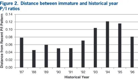
most closely resemble those of the immature year are those with the smallest distances (Years 1988, 1990, and 1991).
Note that the four quarters included in the above calculations contain claim reserve reviews throughout the year. The comparison can be done with more quarters (say 8 or 12) but would lose responsiveness to a changing pattern. On the other hand, using more quarters may increase the stability of the comparison between valuations.
Compared with the latest historical years (1992– 1996), the relatively lower P/I ratios for the imma-ture year suggest that 2010 may have a relatively slower rate of loss payout. This indicates that using a short-term P/I ratio average for the immature year may be sub-optimal.
To quantify these intuitive conclusions, we must establish a “distance” to use to compare the quarterly P/I ratios for each historical year to those observed for the immature year. Historical years whose P/I ratios are closest to those observed in the immature year should be most heavily weighted in the calcula-tion of the average P/I ratio.
In Figure 2, the distances (see formula in section 2) between the immature year and each historical year are displayed. The historical years with P/I ratios that
Table 1. Conversion ratio averages and conversion factors
Conversion Ratio Conversion Factor
1-Year Low 0.8703 1.1490
3-Year Average 0.9331 1.0717
5-Year Average 0.9230 1.0835
5-Year ex-HILO 0.9143 1.0941
10-Year Average 0.9145 1.0935
1-Year High 0.9672 1.0339
Table 2. Historical and immature year P/I ratios
Quarter
Policy Year 21 22 23 24
1987 0.7467 0.7683 0.7808 0.7825
1988 0.7287 0.7426 0.7566 0.7642
1989 0.7018 0.7027 0.7122 0.7225
1990 0.7323 0.7527 0.7676 0.7575
1991 0.7009 0.7211 0.7283 0.7466
1992 0.7439 0.7603 0.7738 0.7822
1993 0.7652 0.7799 0.7893 0.8035
1994 0.7752 0.7865 0.8009 0.8122
1995 0.7694 0.7863 0.7988 0.8075
1996 0.7451 0.7627 0.7767 0.7928
2010 0.7481 0.7333 0.7323 0.7316
Paid-to-Incurred Ratio
0% 10%
1 2 3 4 5 6 7 8 9 10 11 12 13 14 15 16 17 18 19 20
20% 30% 40% 50% 60% 70% 80% 90% 100%
Development Period
period. This is the estimated P/I ratio for the imma-ture year. The inverse of that ratio will be the selected conversion factor.
This method explicitly reflects the expected pay-out pattern of the immature year, while addressing a primary concern with using traditional P/I ratio averaging techniques when determining the paid- to-incurred conversion factor. Also, based on its construction, the Shepard method may produce results that are less volatile when a year with a largely different payout pattern enters the historical development periods.
2.3. Limits of applying Shepard’s method
This section explores two issues that may arise when using Shepard’s method to estimate conversion factors. First, the immature year’s payout pattern may differ from all the historical years. Second, one With the distances above, Shepard’s method3,4 can
be used to assign weights to each of the historical years based on the inverse of their relative distance to the largest distance calculated. The largest distance in Figure 2 is observed in 1994, so it will receive zero weight. Weights for the other historical years are determined using the respective relative dis-tances to the immature year (see Section 2 for addi-tional detail).
Figure 3 presents the weights derived from the distances in Figure 2. The historical years with the smallest distances (Years 1988, 1990, and 1991) receive the most weight.
Using the weights in Figure 3, we calculate a weighted average of the P/I ratios at the conversion
Distance from Recent P/I Pattern 0.00
0.02 0.04 0.06 0.08 0.10 0.12 0.14
'87 '88 '89 '90 '91 '92 '93 '94 '95 '96
Historical Year
Figure 2. Distance between immature and historical year P/I ratios
Prediction Weight
'87 '88 '89 '90 '91 '92 '93 '94 '95 '96
Historical Year
0% 5% 10% 15% 20% 25% 30% 35%
Figure 3. Inverse-distance weights for historical P/I ratios
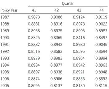
weights will be allocated heavily to the years with the lowest P/I ratios. In this scenario, any average P/I ratio using the historical years will be closer to 1.0000 than it likely should be. The Shepard method conversion factor may still understate true ultimate losses, albeit less so than common averaging tech-niques. The exact weighting of the historical years in Table 3 is shown in Figure 4.
2.3.2. Unstable historical P/I ratio patterns A historical year may have major, abrupt shifts in its P/I ratio over time. This can happen for several reasons, including large claim emergence, low volume sensitive to small claim fluctuations, reopened claims, and large settlements. Providing significant weight to unstable historical P/I ratios may provide non-intuitive results and/or cause large fluctuations in P/I ratio estimates between valuations.
Applying Shepard’s method will control for this if the development quarters used in the distance calculation are those with large shifts in the payout pattern. The squared distance between P/I ratios for the immature year and those in the historical year will be large—resulting in relatively less weight assigned to that historical year’s information. If, instead, the historical year has large shifts after the quarters used in the distance calculation, it may produce an unreasonable P/I ratio estimate. For example, an immature year developed to Quarter 20 will weigh historical years based on Quarters 20 and prior. If or more of the historical payout patterns could be
unstable and unfit for prediction.
2.3.1. Unique P/I ratio pattern
Applying Shepard’s method in this context assumes that the future payout pattern of an imma-ture year will be within the range of those observed in the historical years. When the payout pattern of an immature year is outside the historical range, inverse-distance weighting will heavily weigh one end of the range. This result may not provide a reason-able P/I ratio estimate for the immature year. Treason-able 3 presents an example of this scenario.
In this case, the immature year has comparatively lower P/I ratios than each of the historical years. The Table 3. Historical and immature year (P/I) ratios
Quarter
Policy Year 41 42 43 44
1987 0.9073 0.9086 0.9124 0.9119
1988 0.8831 0.8916 0.8973 0.9022
1989 0.8958 0.8975 0.8995 0.8983
1990 0.8325 0.8365 0.8416 0.8497
1991 0.8887 0.8943 0.8980 0.9045
1992 0.8516 0.8583 0.8595 0.8594
1993 0.8979 0.8983 0.8964 0.8994
1994 0.8934 0.8977 0.8942 0.8963
1995 0.8897 0.8938 0.8921 0.8948
1996 0.8874 0.8906 0.8833 0.8892
2005 0.8095 0.8137 0.8130 0.8115
Prediction Weigh
t
0% 10% 20% 30% 40% 50% 60% 70% 80% 90%
'87 '88 '89 '90 '91 '92 '93 '94 '95 '96
Historical Year
tion period until the point of conversion. If there is a large difference between the estimated value one evaluation period prior to conversion and the actual value at conversion, the ultimate loss projection could change significantly.
To limit the ultimate loss volatility entering the tail development periods, the latest quarterly P/I ratio for the immature year can be weighed with the Shepard’s method estimate. Over the last four quar-ters prior to tail attachment (Quarquar-ters 76–79), the immature year’s latest actual P/I ratio will receive an increasing weight.
The workers compensation portfolio presented in Table 4 (Portfolio 2) demonstrates this conversion factor smoothing.
In this example, the immature year is fully paid out, while all historical years remain active. Any aver-age P/I ratio using these historical years, including one derived with the method described in this paper, will be less than one and would likely overstate the conversion factor and ultimate loss projection. At Quarter 80 and subsequent, the ultimate loss projec-tion will incorporate the actual P/I ratio. This would result in a decrease in ultimate loss in the first tail development period because the applied P/I would be increased.
To minimize any large change in ultimate loss projection, NCCI has implemented a smoothing a historical year closes a large claim in Quarter 30,
Shepard’s method could incorrectly allocate weight based on the slower payout periods.
The risk of volatile payout patterns in conversion factors is not a new problem. The simpler/traditional averaging techniques will include unstable or other-wise unreasonable P/I ratios if they are the earliest available. In the next section, the NCCI approach to identify abrupt changes in historical P/I ratios will be discussed.
2.4. NCCI’s approach to address
the limits of applying Shepard’s method
The following sections will present NCCI’s cur-rent approach to address the previously mentioned limitations of applying Shepard’s method. NCCI’s approach was guided by metrics measuring the predictive accuracy and stability of ultimate loss projections based on NCCI’s workers compensation loss reserving portfolios.
2.4.1. Smoothing conversion factor prediction for unique P/I ratio pattern
As seen in section 1.3.1, when an immature year’s payout pattern is unlike those in historical years, Shepard’s method will provide an estimate at one end of the historical P/I ratio range. This over- or under-estimation will continue for each new
evalua-Table 4. Portfolio 2 P/I ratio patterns
Quarter
Policy Year 73 74 75 76 77 78 79 80
1987 0.9604 0.9612 0.9617 0.9620 0.9629 0.9522 0.9606 0.9850
1988 0.9775 0.9778 0.9772 0.9775 0.9779 0.9783 0.9777 0.9779
1989 0.9060 0.9057 0.9514 0.9397 0.9541 0.9546 0.9554 0.9562
1990 0.8323 0.8341 0.8375 0.8421 0.8442 0.8626 0.8665 0.8870
1991 0.9436 0.9444 0.9458 0.9460 0.9466 0.9474 0.9482 0.9484
1992 0.8616 0.8624 0.8551 0.8584 0.8608 0.8770 0.8789 0.8572
1993 0.8159 0.8175 0.8344 0.8359 0.8347 0.8585 0.8596 0.8644
1994 0.9861 0.9867 0.9867 0.9870 0.9872 0.9875 0.9853 0.9845
1995 0.7635 0.7653 0.7669 0.7709 0.7722 0.7742 0.7762 0.7783
1996 0.9396 0.9403 0.9409 0.9643 0.9649 0.9653 0.9655 0.9660
conversion factor estimation. A stable payout pattern is one that steadily progresses the P/I ratio toward one over time, with limited large changes or reversals. NCCI’s approach to measure payout pattern stability is to fit a curve to the historical P/I ratios and to compare the sum of squared errors to those of the surrounding years.
Figure 5 shows the P/I ratios for a historical year (1988) that contains a noticeable shift at Quarter 74. A logarithmic curve was fit to these ratios to recog-nize that P/I ratios generally increase to unity at a decreasing rate. The fit uses the latest four develop-ment years (16 quarters) to mitigate against large changes commonly observed in early quarters and for easier curve-fitting.
Table 6 displays the results of fitting curves to the P/I ratios for 10 historical years. If one historical year has a relatively large percentage of the total sum of squared errors observed across the entire 10-year historical period, it may suggest that that year is procedure beginning four evaluations prior to the
point of conversion, quarter 80. A demonstration of this can be seen in Table 5.
The final conversion—which includes weighting the Shepard method result with the latest actual P/I ratio—spreads the total impact of the incurred value change across each valuation quarter. The percent-age sliding scale is a judgmental selection. Four quarters are smoothed because the P/I ratio is not expected to change much prior to Quarter 80. The earlier the smoothing is applied, the more likely the final estimated conversion factor is overstated. Using the Shepard conversion alone would result in a 2% decrease in ultimate loss at Quarter 80, caused entirely by the conversion factor.
2.4.2. Removing unstable historical P/I ratio patterns
In section 1.3.2, we discussed the impact that unstable historical P/I ratio patterns can have on Table 5. Conversion factors by valuation
Valuation Quarter QTRs Used Shepard P/I Ratio(1) Latest P/I Ratio(2) Shepard Weight(3) (4) = (1)
p (3) + (2) p [1 – (3)]
Final Conversion Ratio
(5) = 1/(4) Final Conversion
Factor
12/31/2015 73–76 0.9812 1.0000 100% 0.9812 1.0192
3/31/2016 74–77 0.9810 1.0000 75% 0.9858 1.0145
6/30/2016 75–78 0.9804 1.0000 50% 0.9902 1.0099
9/30/2016 76–79 0.9798 1.0000 25% 0.9950 1.0051
P/I rati
o
0.85 0.88 0.90 0.93 0.95
65 66 67 68 69 70 71 72 73 74 75 76 77 78 79 80
Quarter
which are represented by periods of development time. The focal point of this application will be the inverse-distance weighting formula that determines which surrounding points are most similar to the one being estimated. The surrounding points, in this context, will be the P/I ratios for years that have reached the point of conversion. The estimated point will be the (unknown) P/I ratio at conversion for the immature year.
This method is simple to implement and efficient to calculate.
The conversion ratio is estimated at a selected tail attachment point. Ultimate losses for an immature year are estimated by developing observed paid losses with the product of paid link ratios prior to the tail attachment point, the conversion factor, and an incurred loss tail factor. To begin, we define:
Ps,i Paid loss value at year s and devel-opment time i
fi,A Paid cumulative development factor for development from time i to tail factor attachment point A
Is,i Incurred loss value at year s and development time i
, ,
,
Q P
I
s i s i s i =
Observed P/I ratio at year s and
development time i
Qˆs,A Estimated conversion ratio at year s and the tail factor attachment point A
Ts,A Incurred tail factor for loss valued at year s and tail factor attachment point A ˆ , , , R T Q s A s A s A =
Implied paid tail factor for year s at development time A
An ultimate loss projection is defined:
. .
., , ,
ULs=Ps i fi A Rs A
The major assumption for actuarial use is that the historical payout patterns are relevant to the patterns of the immature years. It is up to the discretion of the actuary to judge the reasonableness of this notably less stable than the others; in this case, NCCI
reduces the weight factor calculated using Shepard’s method to zero. This is accomplished by incorporat-ing a penalty factor that is either one (stable year) or zero (unstable year). After a review of accuracy and stability metrics using several percentage thresholds, NCCI chose a threshold of 40%. This resulted in pre-dictions that were largely unbiased, more accurate, and provided stability of ultimate loss projections between valuations.
Historical year 1988 is shown in Figure 5. While this was the least stable of the historical years, it did not comprise more than 40% of the total error and, therefore, was not excluded from the distance-weighting method.
3. Theory and formulas
In this section, we will outline the general formulas for applying Shepard’s method to estimate conver-sion factors.
Shepard’s method was initially created to inter-polate points in irregularly spaced data to create smooth surface models.5 This was done with a
two-dimensional space and could be generalized for a three-dimensional space. In our case, we will generalize the method to any number of dimensions, Table 6. Logarithmic fit parameters and residual value
Policy Year
Logarithmic Fit
RSS % Total Penalty Factor
a b
1987 –0.1965 1.7651 0.0006 18.3% 1
1988 0.1514 0.2680 0.0011 32.5% 1
1989 0.0872 0.5165 0.0000 1.3% 1
1990 0.0668 0.5875 0.0005 13.0% 1
1991 –0.0638 1.1896 0.0001 3.1% 1
1992 0.0438 0.6797 0.0005 12.8% 1
1993 0.1077 0.4620 0.0002 5.2% 1
1994 –0.0255 1.0445 0.0002 5.8% 1
1995 0.1225 0.3706 0.0002 6.3% 1
1996 0.0444 0.7744 0.0001 1.6% 1
This application of Shepard’s method provides a specific Qˆ value for each of the years at develop-ment periods prior to the tail attachdevelop-ment point. The favorable characteristics of Shepard’s inverse-distance weighting to estimate P/I ratios include:
1. The weighting of P/I ratios will be limited to those in the portfolio’s history.
2. Distance formulas provide an intuitive recognition of historical payout patterns that resemble those observed in the immature year.
3. Distance formulas are efficient to calculate and easy to implement.
4. Inverse-distance interpolation can be applied to any number of dimensions, i.e., development periods.
5. Distance formulas that include multiple develop-ment periods capture the direction of the payout pattern, or whether the P/I ratio is currently moving closer to or farther from unity.
6. Euclidean distance7 provides greater penalties
to volatile historical patterns than Manhattan dis-tance,8 though any distance function can be used.
7. The number of development periods used in the distance formula should be low, avoiding issues with Euclidean distances in high-dimensional analysis.9
8. Shepard’s weighting formula can be imple-mented across multiple portfolios without further assumptions.
9. Shepard’s method is distribution-free.
4. Complete example and results
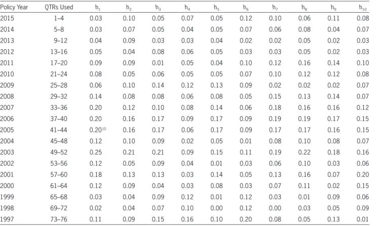
In this section, we will provide a full example esti-mating conversion factors for the initial example portfolio above. For the sake of brevity, the triangle of P/I ratios is suppressed. Table 7 shows the distances assumption. Dramatic changes in claim payoutprac-tices may result in distortions. This is similarly true for chain-ladder methods.
Now, we can present the formulas for applying Shepard’s method to P/I ratio prediction. The first step in applying Shepard’s method is to calculate the distance between P/I ratios for the more immature years and those in the historical years for all s and t:
, , ,
2
max 1 max
hs t Qs x Qt x
x i t n i t
∑
(
)
= − ( ) ( ) ( ) = − −where hs,t represents a distance calculated using n development time periods.6 This is calculated for
each of the N historical years, s, and a fixed imma-ture year t.
After the distances have been calculated, weight factors are derived for all s:
.
, ,
, 2
W R h
R h
s t s t s t
= −
where R = max(h1,t, . . . , hN,t).
The incorporation of penalty factors, Ps, as dis-cussed in section 1.4.2, can be used to produce adjusted weights that are rescaled to sum to unity:
w W xP
W xP
s t s t s s t s s N
∑
= = , , , 1The final estimated P/I ratio is then calculated as
.
ˆ .
, 1 , ,
Qt A s ws t Qs A
N
∑
= =
As noted in section 1.4.1, the final conversion ratio may be adjusted to limit the influence of his-torical ratios when immature years’ payout patterns appear largely different than the range observed in the historical years.
6The operator, |, restricts the summation to the development times, i,
conditioned on a given year, t.
7Euclidean distance (L
2) is defined as d(x, y) = (x1−x2)2+(y1−y2)2. 8Manhattan distance (L
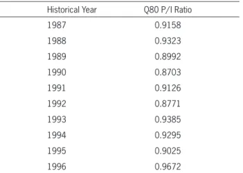
These weights are then applied to the histori-cal year P/I ratios at Quarter 80 shown in Table 10, providing an estimated P/I ratio for each immature year. With the estimated Quarter 80 P/I ratios, we can calculate the final conversion factors. The pay-out patterns near the conversion development period were within historical ranges, so smoothing was unnecessary.
The boundaries of potential conversion factors (see Table 1) suggest a 3%–15% increase to the paid projection at Quarter 80. In Table 11, we can see that applying Shepard’s method to weigh the historical years’ P/I ratios allows the full range of potential factors to be applied to the differing payout patterns. In contrast, using various averages of historical P/I ratios (see Table 1) would produce results similar to Shepard’s method in only a few years, potentially overstating or understating losses in most years.
To expand on these results, we can look across mul-tiple portfolios. A retrospective test was performed between the P/I ratios for each immature year and
each of 10 historical years. The distances rely on the most recent four P/I ratios. An example in policy year 2005 is calculated in a footnote.
Next, we will show the R values, which are the maximal h values for each row above. With these, we can calculate the weighting factors.
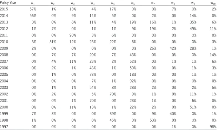
At this point, the actuary may apply a penalty factor for unstable historical years that are unfit for prediction. For this data, no outlying historical years exceeded the 40% error tolerance described in sec-tion 1.4.2, and therefore no penalty factors were used. In Table 9, we show the inverse-distance weights calculated using the weighting factors in Table 8. Note that all rows sum to 100% but may display otherwise due to rounding.
Table 7. Four-dimensional distances
Policy Year QTRs Used h1 h2 h3 h4 h5 h6 h7 h8 h9 h10
2015 1–4 0.03 0.10 0.05 0.07 0.05 0.12 0.10 0.06 0.11 0.08
2014 5–8 0.03 0.07 0.05 0.04 0.05 0.07 0.06 0.08 0.04 0.07
2013 9–12 0.04 0.09 0.03 0.03 0.04 0.02 0.02 0.05 0.02 0.03
2012 13–16 0.05 0.04 0.08 0.06 0.05 0.03 0.03 0.05 0.02 0.03
2011 17–20 0.09 0.09 0.01 0.05 0.04 0.10 0.12 0.16 0.14 0.10
2010 21–24 0.08 0.05 0.06 0.05 0.05 0.07 0.10 0.12 0.12 0.08
2009 25–28 0.06 0.10 0.14 0.12 0.13 0.09 0.02 0.02 0.02 0.07
2008 29–32 0.14 0.08 0.08 0.06 0.08 0.05 0.15 0.13 0.14 0.07
2007 33–36 0.20 0.12 0.10 0.08 0.14 0.06 0.18 0.16 0.16 0.12
2006 37–40 0.20 0.16 0.17 0.09 0.17 0.09 0.19 0.19 0.17 0.15
2005 41–44 0.2010 0.16 0.17 0.06 0.17 0.09 0.17 0.17 0.16 0.15
2004 45–48 0.12 0.10 0.09 0.02 0.05 0.01 0.08 0.10 0.08 0.07
2003 49–52 0.25 0.21 0.21 0.09 0.15 0.11 0.19 0.22 0.18 0.16
2002 53–56 0.12 0.05 0.09 0.04 0.01 0.03 0.06 0.10 0.03 0.06
2001 57–60 0.18 0.13 0.13 0.03 0.14 0.05 0.13 0.16 0.07 0.20
2000 61–64 0.12 0.09 0.04 0.03 0.08 0.03 0.07 0.11 0.02 0.15
1999 65–68 0.03 0.04 0.09 0.12 0.01 0.12 0.03 0.01 0.09 0.06
1998 69–72 0.02 0.04 0.07 0.10 0.00 0.12 0.00 0.03 0.05 0.09
1997 73–76 0.11 0.09 0.15 0.16 0.10 0.20 0.08 0.05 0.13 0.01
10Using data in Table 3 for policy year 2005,
0.20 .9073 .8095 .9086 .8137 .9124 .8130 .9119 .8115 .
1
2 2
2 2
h ( ) ( )
( ) ( )
= = − + −
Table 8. Shepard’s method weighting factors
Policy Year R W1 W2 W3 W4 W5 W6 W7 W8 W9 W10
2015 0.12 476 5 109 35 140 0 3 55 1 14
2014 0.08 512 1 82 130 44 1 16 0 131 3
2013 0.09 149 0 309 600 219 1,071 886 75 1,964 311
2012 0.08 39 220 0 25 49 310 638 65 1,626 350
2011 0.16 27 29 6,198 184 408 16 4 0 1 14
2010 0.12 20 183 73 135 128 34 2 0 0 17
2009 0.14 96 7 0 1 0 15 1,075 1,761 1,188 63
2008 0.15 0 33 36 101 35 215 0 2 0 72
2007 0.20 0 10 25 49 5 111 0 2 1 13
2006 0.20 0 1 1 37 1 43 0 0 1 2
2005 0.20 0 1 1 150 1 35 1 1 1 2
2004 0.12 0 1 4 1,559 110 19,257 14 3 11 30
2003 0.25 0 1 1 47 7 24 2 0 2 4
2002 0.12 0 119 10 270 3,813 485 67 3 586 68
2001 0.20 0 6 8 904 4 293 8 1 73 0
2000 0.15 2 20 437 524 42 881 62 7 2,052 0
1999 0.12 681 330 8 0 3,867 0 865 3,962 7 72
1998 0.12 1,126 319 47 2 47,342 0 56,602 513 124 10
1997 0.20 19 40 3 1 22 0 49 218 7 21,390
Table 9. Shepard’s method weights
Policy Year w1 w2 w3 w4 w5 w6 w7 w8 w9 w10
2015 57% 1% 13% 4% 17% 0% 0% 7% 0% 2%
2014 56% 0% 9% 14% 5% 0% 2% 0% 14% 0%
2013 3% 0% 6% 11% 4% 19% 16% 1% 35% 6%
2012 1% 7% 0% 1% 1% 9% 19% 2% 49% 11%
2011 0% 0% 90% 3% 6% 0% 0% 0% 0% 0%
2010 3% 31% 12% 23% 22% 6% 0% 0% 0% 3%
2009 2% 0% 0% 0% 0% 0% 26% 42% 28% 1%
2008 0% 7% 7% 20% 7% 43% 0% 0% 0% 14%
2007 0% 4% 11% 23% 2% 52% 0% 1% 1% 6%
2006 0% 2% 1% 43% 1% 50% 0% 0% 1% 3%
2005 0% 1% 0% 78% 0% 18% 0% 0% 1% 1%
2004 0% 0% 0% 7% 1% 92% 0% 0% 0% 0%
2003 0% 1% 1% 54% 8% 28% 2% 0% 2% 5%
2002 0% 2% 0% 5% 70% 9% 1% 0% 11% 1%
2001 0% 0% 1% 70% 0% 23% 1% 0% 6% 0%
2000 0% 0% 11% 13% 1% 22% 2% 0% 51% 0%
1999 7% 3% 0% 0% 39% 0% 9% 40% 0% 1%
1998 1% 0% 0% 0% 45% 0% 53% 0% 0% 0%
on a mix of small, medium, and large workers com-pensation portfolios. P/I ratios were estimated using various averaging methods and Shepard’s method for all available years. In Figure 6, we summarize the distributions of squared error percentage values in these estimates across methods. In the error formula on the y-axis, “A” represents the actual P/I ratio at Quarter 80 and “E” represents the expected P/I ratio in prior periods based on the method on the x-axis. Table 10. Quarter 80 P/I ratios
Historical Year Q80 P/I Ratio
1987 0.9158
1988 0.9323
1989 0.8992
1990 0.8703
1991 0.9126
1992 0.8771
1993 0.9385
1994 0.9295
1995 0.9025
1996 0.9672
Table 11. Conversion ratios and conversion factors
Policy Year Conversion RatioShepard Conversion FactorShepard
2015 0.9131 1.0952
2014 0.9064 1.1033
2013 0.9044 1.1057
2012 0.9164 1.0912
2011 0.8995 1.1117
2010 0.9071 1.1025
2009 0.9242 1.0820
2008 0.8968 1.1151
2007 0.8874 1.1268
2006 0.8784 1.1385
2005 0.8739 1.1443
2004 0.8770 1.1403
2003 0.8829 1.1326
2002 0.9076 1.1018
2001 0.8747 1.1433
2000 0.8932 1.1195
1999 0.9230 1.0834
1998 0.9266 1.0792
1997 0.9666 1.0346
(A–E)^2 /
A
0.0000 0.0025 0.0050 0.0075 0.0100
3YR 5xHL 5YR 10YR Shepard
Method
Acknowledgments
I would like to express my gratitude to several people who made my research successful:
My manager, Ia Hauck, and the NCCI Actuarial & Economic Services Division’s leadership for sup-porting my research into this topic, as well as helping me present it at multiple actuarial forums.
Damon Raben, for his extensive review and sugges-tions throughout the research, writing, and presentation processes. He consistently challenged and improved my work.
Jay Rosen, Barry Lipton, Kirt Dooley, Sean Cooper, and Erik Miller for their assistance in the final stages of editing and review of the paper.
All the members of the Actuarial Reserving team, who helped to not only review but also implement this new method at NCCI.
References
Aggarwal, C. C., A. Hinneburg, and D. A. Keim, “On the Surprising Behavior of Distance Metrics in High Dimensional Space,” Database Theory—ICDT 2001 Lecture Notes in Computer Science, 2001, pp. 420–434.
CAS Tail Factor Working Party. “The Estimation of Loss Devel-opment Tail Factors: A Summary Report,” Casualty Actuarial Society E-Forum, Fall 2013, pp. 17–25.
Franke, R., and G. Nielson, “Smooth Interpolation of Large Sets of Scattered Data,” International Journal for Numerical Methods in Engineering 15: 11, 1980, pp. 1691–1704. Franke, R., “Scattered Data Interpolation: Tests of Some
Methods,” Mathematics of Computation 38: 157, 1982, pp. 181–200.
Shepard, D., “A Two-Dimensional Interpolation Function for Irregularly-Spaced Data,” Proceedings of the 1968 23rd ACM National Conference, 1968, pp. 517–523.
The box plots condensed closest to zero suggest the greatest predictive accuracy.
The results of the Shepard method are superior to every averaging method presented, with a reduced median and maximum error.
5. Conclusion
When using paid loss chain-ladder methods to estimate ultimate losses, an incurred loss tail factor can be used with a paid-to-incurred conver-sion factor to convert developed paid losses to an incurred basis. This implies a paid tail factor from a combination of the incurred factor and the year’s loss payout pattern. We showed that relying on common averaging techniques of the most recent historical years’ P/I ratios may not appropriately reflect the payout pattern of the relatively immature years. Also, large unwarranted changes in P/I esti-mates may arise when a new year enters the historical averages.