Research Note
Three-Dimensional Data Transfer
Operators in Plasticity Using SPR
Technique with C
0
, C
1
and C
2
Continuity
A.R. Khoei
1;and S.A. Gharehbaghi
1In this paper, the data transfer operators are developed in three-dimensional elasto-plasticity using the Superconvergent Patch Recovery (SPR) method. The transfer operators are dened for mapping of the state and internal variables between dierent meshes. The internal variables are transferred from Gauss points of old mesh to the nodal points. The variables are then transferred from the nodal points of old mesh to the nodal points of new mesh. Finally, the values are computed at the Gauss points of new mesh using their values at the nodal points. Aspects of the transfer operators are presented in a three-dimensional superconvergent path recovery technique, based on C0, C1 and C2 continuity. Finally, the eciency of the computational algorithms is demonstrated using a circular tube subjected to internal pressure.
INTRODUCTION
In a large class of nonlinear problems, the optimal mesh conguration changes continuously throughout the deformation process requiring data transfer during analysis. In addition to data transfer, error estimation procedures play a crucial role in quality assurance by providing a reliable nite element solution to be used as a basis for the industrial decision-making process. In fact, the error estimation leads to an optimum mesh conguration, which can be used as a new mesh for the data transfer at any step of the analysis. Error estimation and data transfer have been extensively performed in 2D elasticity problems [1-6]. Among numerous contributions, the basic ideas and numerical strategies are introduced in [7-10]. On the contrary, although some advances have been recorded for certain classes of nonlinear problem [9], there is very little published work on adaptive strategies for history-dependent nonlinear problems in solid mechan-ics. Notable exceptions are contributions by Johnson and Hansbo [11], Ladeveze et al. [12], Samuelsson and Wiberg [13] and Lee and Bathe [14].
The Superconvergent Patch Recovery (SPR)
1. Center of Excellence in Structures and Earthquake Engi-neering, Department of Civil EngiEngi-neering, Sharif Univer-sity of Technology, P.O. Box 11155-9313, Tehran, Iran. *. To whom correspondence should be addressed. E-mail:
method was rst introduced by Zienkiewicz and Zhu [1-3]. In the SPR method, a continuous and accurate stress can be obtained over the entire domain by the recovery of nodal stresses. The nodal stresses are evaluated by determining a polynomial expansion over a patch of elements sharing the node, which t the raw FEA results in a set of sampling points inside the patch in a least square manner. In the original SPR method, the superconvergent points are used as sampling points. As the stress information is only available at the integration points, these points are then used as sampling points to recover the stresses in history dependent problems [15]. Gu et al. [16] modied the original SPR method to capture more accurate results. An application of the SPR technique was implemented in liquefaction problems by Tang and Sato [17].
In the present paper, the SPR method is extended to three-dimensional nonlinear problems, based on C0, C1and C2 continuity. The technique is then employed to transfer the variables from the old mesh to a new one. The procedure of data transfer is performed in three dierent stages by transferring the internal variables from old Gauss points to old nodal points, the mapping of variables from old nodal points to new nodal points and, nally, transferring the new nodal points to new Gauss points. The eects of each variant of C0 , C1 and C2 continuity are investigated using the relevant estimated error. It is shown how the new algorithm of the 3D SPR technique can be applied to
accurately recover the stresses. Finally, a circular tube, subjected to internal pressure, is analyzed, in order to demonstrate the performance of the 3D SPR method in nonlinear problems using tetrahedral meshes. 3D DATA TRANSFER OPERATORS
In a non-linear adaptive procedure, one usually starts from a mesh with a reasonable distribution of elements. The non-linear analysis will be carried out at dierent load steps until the estimated error exceeds the pre-scribed value. At this time, a new mesh is generated using an appropriate renement criterion. The non-linear analysis must be performed on the new mesh starting from the beginning of the load step (i.e. load step n). In this case, the information at the end of the previous load step (load step n 1) must be transferred to the new mesh. Since this information is history dependent, the data transfer between the old and new meshes is one of the most challenging parts of nonlinear analysis. It is important that the transfer of information from old to new meshes is achieved with minimum discrepancy in equilibrium and constitutive relations.
Ortiz and Quigley [18] developed a, so-called, consistent transfer operator, using an appropriate Hu-Washizu functional. The method simply implements a discontinuous distribution of history dependent pa-rameters using local interpolation functions. These functions are chosen so that the interpolated eld results in exact values at the integration points. This was achieved by employing the local shape functions having unit values at integration points. In other words, the method is performed based on the interpo-lation of values at the integration points when the new Gauss points (in new mesh) are inside the group of old Gauss points in a particular element and extrapolating the values when the new Gauss point is outside the group of old Gauss points but not outside the old element. Clearly, the discontinuity of the eld along the boundaries of elements creates some diculties in the evaluation of values at those new Gauss points located on the element edges. In order to solve the problem, a specic form of remeshing has been applied, using the Delaunay triangulation. In this case, the old element is divided into smaller elements, so that the new Gauss points will always be inside the group of old ones in the old element. However, the methodology of data transfer fails when a general new mesh is used [19,20]. A similar procedure has been employed by Lee and Bathe [14] and Peric et al. [21]. In this approach, the history dependent variables in the old mesh are rst projected to nodal points. The values of new nodal points in the new mesh are then computed by the simple interpolation of old nodal values, using the shape-functions. In order to have a self-consistent
condition, Lee and Bathe [14] transferred only a few parameters between two meshes, i.e. the eective plastic strain and trial elastic deformation gradients, while the other parameters are computed from the con-stitutive relation. A similar procedure was performed by Peric et al. [21], where the transferred value of displacements at the end of load step n in the old mesh is considered a trial solution of the new mesh for load step n. There is an argument about the necessity of self-consistency of the history dependent parameters in the last two approaches. In fact, by transferring the information to the nodes and recalculating them at new Gauss points, the equilibrium of the system will be violated. In fact, even if the mesh is not changed, the above procedure will violate the equilibrium of the system. It is worthwhile to note that, even in elastic solutions, the elastic constitutive relations are approximately satised in order to achieve a more accurate solution.
In this study, the two-dimensional Supercon-vergent Patch Recovery (SPR) method presented by Khoei et al. [22,23] is extended to three-dimensional plasticity problems with several improvements, which demonstrates its capability of recovering data from Gauss points to nodal points. Firstly, it is necessary to represent two concepts related to the mapping of internal variables between two nite element meshes, called M1 and M2. This mapping is an essential part of any adaptive strategy employed in the simulation of history-dependent material processes on evolving general unstructured meshes. The mapping of internal variables is formally denoted by the transfer operator, T1. In addition, a transfer operator is employed that transfers the displacement eld from the old to a new mesh. In the context of the backward Euler scheme, where a solution is sought at time instant tn+1, this transfer provides a trial solution. The mapping of displacement is formally denoted as transfer operator T2.
Let uM1
n , "M1n ,P"M1n , nM1, qnM1, denote values of the displacement, strain tensor, plastic strain tensor, stress tensor and a vector of internal variables at time tn for the mesh M1 (Box 1). For simplicity of notation, a state array, M1
n = (uM1n ; "M1n ;P"M1n ; nM1; qnM1) is dened. Furthermore, let it be assumed that the
estimated error of solution M1
n respects the prescribed criteria, while these are violated by the solution M1
n+1. In this case, a new mesh, M2, is generated and a new solution, M2
n+1, needs to be computed. As the backward Euler scheme is adopted here, the plastic strain,p"M2
n , and the internal variables, qnM2, for a new mesh, M2, at time tn, need to be evaluated. In this way, the state, ~M2
n = (P"M1n ; qnM1), is constructed, where the symbol, , is used to denote a reduced state array. It should be noted that this state characterizes the history of the material and, in the case of a fully implicit scheme, provides sucient information for the computation of a new solution, M2
n+1. Data Transfer Operator T1
Consider T1to be the transfer operator between meshes M1 and M2, dened by:
(p"M2
n ; qM2n ) = T1(p"M1n ; qnM1): (1) The variables, (p"M1
n ; qnM1), specied at quadrature points of the mesh, M1 are transferred by the operator, T1, to any point in domain . In order to evaluate the variables, (p"M2
n ; qM2n ), at the quadrature points of the new mesh, M2, the operator, T1, can be constructed in dierent ways. Firstly, a simple version of the transfer operator may be constructed by taking constant values over the area associated with each quadrature point. Note that this construction is local. Secondly, it is possible to construct a solution, which is continuous, for instance, using a least-square method, or a suitable projection ofp"M1
n , which satises the following: Z
F [( P "M1
n ;qM1n ) (P"M1n ; qM1n )]dx = 0; (2) where F is the so-called projection matrix. This type of transfer operator can be global or local. In this study, a local transfer method is dealt with, which is simple and, of course, general in application.
The basic steps of the implementation procedure, which is applicable for any type of nite element mesh, are described as follows. The continuous plastic strain tensor, p"M1
n , and the internal variable vector, qM1
n , are obtained by projecting the Gauss point components, p"M1
n;G and qM1n;G, to the nodal points, i.e., p"M1
n;N and qM1n;N. In order to project the values of Gauss points to nodal points, three variants of the 3D SPR method are applied here, as described in the following section. The nodal values of the plastic strain tensor, p"M1
n;N, and the internal variable vector, qM1n;N, of mesh M1 are then transferred to the nodes of the new mesh, M2, resulting in components, p"M2
n;N, and the internal variable vector, qM2
n;N. The values of the Gauss points in the new mesh, M2, i.e.,p"M2
n;G and qn;GM2, are nally
obtained by interpolation, using the shape functions of the nite elements. The described transfer operation, T1, is schematically presented in Box 2.
Data Transfer Operator, T2
In the context of the backward Euler scheme, with a strain driven format and Newton-Raphson iterative procedure, the transferred displacement eld on a new mesh is used to provide an initial guess (trial solution) for the displacements at the rst iteration of the Newton-Raphson scheme. Hence, the transfer operator, T2, can be dened as:
trialuM2
n+1= T2(uM1n+1): (3)
It means that the trial displacement eld, trialuM2 n+1, can be evaluated by transfer of the displacement eld, uM1
n+1, from the mesh, M1, at time step tn+1. For convenience, a schematic diagram of transfer operator T2 is presented in Box 3. It is important to note that the transfer operator, T2, corresponds to transfer of the displacement eld, uM1
n+1, which is fully described by the nodal values and nite element interpolation functions. Therefore, the same transfer operator, T2, can be used to transfer the displacements and internal
Box 2. The transfer operator T1.
state variables from the nodal points of the old mesh to the nodal points of the new mesh.
3D SUPERCONVERGENT PATCH RECOVERY METHOD
The concept of superconvergence is that, at some points, the approximate solutions are more accurate, or, in other words, the rate of convergence at those points is higher than those of other points. The existence of these points for each element has been discussed in [24] and can be proved by using the relationship between the exact and FEM solutions. Rewriting the governing equation of the system, it can be seen that there is an important relation between the FEM solution and the associated errors as:
Z B
Te
d = 0; (4)
where e is the error of stress and B has its con-ventional denition in FEM formulation. The FEM solution satisfying the above equation minimizes the error of energy dened as:
e= Z
(
h)T(" "h)d 1
2
; (5)
where h and are the FEM and recovered stress elds at the end of time step n, "h = B(un un 1), and " is the recovered incremental strain eld. Now, consider an exact solution with only one order higher than that of shape-functions. From the above statement, it can be concluded that the FFM solution must be exact at least at one (or more) location. In one-dimensional problems, these points can be located easily and it has been shown that the gradients of Gauss quadrature points, used for reduced integration, are superconvergent. In two or more dimensional problems and only for very simple elements, like rectangular elements, it can be shown that the Gauss points used for reduced integration are superconvergent points [25,26].
To construct the gradient eld, one simply writes the new eld as a polynomial with unknown coe-cients, namely, for each component;
= a
0+ a1x + a2y + a3z + + anzn = [1; x; y; z; ; zn][a
0; a1; a2; ; an]T
= P a: (6)
Now, a norm of the dierence between the new eld and the values at superconvergent points are minimized with respect to a as:
=N.S.X i=1
(Pia (hs)i)2; (7)
where (s
h)i represents the gradient at sampling point i with its coordinates (xi, yi, zi). The local coordinate, together with normalized values, with respect to the maximum and minimum dimensions of the patch, is usually used. The minimization process leads to:
a =hXPT i Pi
i 1hX PT
i (sh)i i
: (8)
Having obtained the polynomial coecients, the nodal values can simply be evaluated, as follows:
= P
nodea: (9)
The above procedure can be applied for each vertex of the domain. For quadratic elements with edge points, the gradients are computed by averaging the results of the patches at the side vertices on the edge. As the new eld of gradient is superconvergent, it follows that the new eld must reproduce the exact gradient eld of a problem with an exact solution one order higher than the FEM solution. It is worthwhile to note that the superconvergent property only exists at the position of the sampling points. In the following simple example, it can be shown that the above mentioned procedure, using ordinary integration points, does not give superconvergent answers:
=N.G.X i=1
(Pia (gh)i)2; (10)
where N.G. is the total number of integration points in the patch. As mentioned before, if the exact solution is only one order higher than the FEM solution, the SPR procedure can exactly recover the exact eld. On the other hand, the recovered solution using ordinary inte-gration points cannot reproduce the exact eld, which means that the recovered eld is not superconvergent. It must be mentioned that, although minimization of the following functional in integral form gives answers independent from the number of Gauss points used, it will not result in a superconvergent eld of stresses.
= Z
P
(P a h)2d: (11)
In fact, the functional form of the above equation is the general form of Relation 10, considering appropriate weights for each integration point. In this case, the worst situation happens when the relative length of the two elements in the patch is near to zero (or innity). In this situation, the recovered eld of stress is the same as the FEM solution of the larger element. In a computer-based method, it has been proved that the SPR recovery method gives the most robust error estimation, compared to all other kinds (residual type or etc.) [25,26].
In what follows, the 3D superconvergent path recovery method is illustrated, using three variants based on C0, C1 and C2 continuity. The algorithm is illustrated for both the interior and boundary nodes and the eciency of each variant is described.
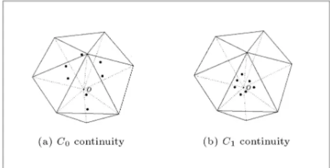
Variant of C0 Continuity
After nite element analysis, a patch is dened for each vertex node inside the domain by the union of elements sharing the node. At each node of the interior patch center, the connected tetrahedral elements, along with their nodes and Gauss points, are obtained, as shown in Figures 1 and 2. In order to perform the polynomial expansion (Equation 6), the Gauss points of a particular patch are determined, as shown in Figure 3. For nodes of the boundary patch center, the connected elements and the nearest connected interior nodes to the center of the patch, together with corresponding elements of that patch, are obtained, as shown in Figure 4. For the 3D SPR method with C0 continuity, the polynomial expansion (Equation 6) can be represented in its simplest form as follows:
= a
0+ a1x + a2y + a3z
= [1; x; y; z][a; a1; a2; a3]T = P a: (12) It can be seen from the above relation that the algorithm has C0 continuity. For a three-dimensional mesh with tetrahedral elements, the SPR patch can
Figure 1. The connected elements at each node for interior patch center.
Figure 2. The Gauss points of connected elements.
Figure 3. The Gauss points for a particular patch.
Figure 4. The connected elements at each node for boundary patch center.
be constructed, based on the procedure described in Tables 1 and 2, for the interior and boundary nodes, respectively. Clearly, in C0continuity, some additional eorts are necessary to be taken into account for boundary nodes, as there may not be enough Gauss points for a particular patch. In this case, a modied algorithm of C0 continuity employed for interior nodes can be applied for boundary nodes, as presented in Table 2.
Variant of C1 Continuity
In order to construct the gradient eld of C1continuity, a polynomial of second order can be considered, as follows:
= a
0+ a1x + a2y + a3z + a4x2+ a5y2 + a6z2+ a7xy + a8yz + a9zx
=[1; x; y; z; x2; y2; z2; xy; yz; zx][a
0; a1; a2; ; a9]T
= P a; (13)
in which ten Gauss points are necessary to construct the curve for a particular patch. In this case, if there are not enough Gauss points for a particular patch, some additional eort must be taken into account, as illustrated in Tables 3 and 4.
Table 1. The SPR algorithm of C0 continuity for interior nodes.
1. Obtain the connected elements at each node for interior patch center, as shown in Figure 1, 2. Determine the nodes of elements obtained in step 1,
3. Obtain the Gauss points of elements indicated in step 1 as shown in Figure 2, 4. Let NGAUS be equal to the number of elements of the patch.
Now, if NGAUS = 1, then use all Gauss points for SPR method otherwise, if NGAUS = 2 use the rst 2*NGAUS nearest Gauss points to the patch center else, nd
the NGAUS nearest Gauss points to the patch center, as shown in Figure 3. Set the CRITICAL NODE ag to TRUE, if there are not
enough Gauss points for this patch. Use simple averaging or other methods for CRITICAL NODES,
5. Normalize all nodes with respect to minimum and maximum coordinates, in order to construct a localcoordinate system for the patch,
6. Obtain all corresponding coecients for the stress and strain components using Equation 12, 7. Finally, calculate the stress and strain components at the center of the patch based on the best tting curve in step 6.
Table 2. The SPR algorithm of C0 continuity for boundary nodes.
1. Obtain the connected elements at each node for boundary patch center, as shown in Figure 4, 2. Determine the nearest connected interior node (to the center of patch) and add all corresponding elements of that patch to those elements obtained in step 1,
3. If step 2 fails, obtain the nearest interior node and add all corresponding elements of that patch to those elements obtained in step 1,
4. If steps 2 and 3 fail, obtain the nearest connected boundary node and add all connected elements of that node to those elements obtained in step 1,
5. If steps 2, 3 and 4 fail, obtain the nearest boundary node and add all connected elements of that node to those elements obtained in step 1,
6. If steps 2 to 5 fail, or there are not enough Gauss points for this patch, set the ag for this node to CRITICAL NODE. Use simple averaging or other methods for CRITICAL NODES,
7. Determine the nodes of elements obtained in previous step (Figure 1),
8. Obtain the Gauss points of elements indicated in previous step, as shown in Figure 2, 9. Let NGAUS be equal to the number of elements of the patch. Now, if NGAUS = 1,
then use all Gauss points for SPR method, otherwise if NGAUS = 2 use the rst 2*NGAUS nearest Gauss points to the patch center else, nd the NGAUS nearest Gauss points to the patch center, as shown in Figure 3,
10. Normalize all nodes with respect to minimum and maximum coordinates, in order to construct a local coordinate system for the patch,
11. Obtain all corresponding coecients for the stress and strain components using Equation 12,
12. Finally, calculate the stress and strain components at the center of the patch based on the best tting curve in previous step.
Table 3. The SPR algorithm of C1 and C2 continuity for interior nodes.
1. Obtain the connected elements at each node for interior patch center, as shown in Figure 1, 2. Determine the nodes of elements obtained in step 1,
3. Obtain the Gauss points of elements indicated in step 1, as shown in Figure 2,
4. Let NGAUS be equal to the number of elements of the patch, which is multiplied by 1 (or 3) for C0
(or C1) tetrahedral elements. If NGAUS < 9, then use all Gauss points for the SPR method, otherwise
obtain the NGAUS nearest Gauss points to the patch center (Figure 3). Set the CRITICAL NODE ag to TRUE, if there are not enough Gauss points for this patch. Use simple averaging or other methods for CRITICAL NODES. It is important to note that one can enhance this method with a better approach based on the C0 variant for CRITICAL NODES,
5. Normalize all nodes with respect to minimum and
maximum coordinates, in order to construct a local coordinate system for the patch,
6. Obtain all corresponding coecients for the stress and strain components using Equation 13 for C1
continuity, or Equation 14 for C2 continuity,
7. Finally, calculate the stress and strain components at the center of the patch based on the best tting curve in step 6.
Table 4. The SPR algorithm of C1and C2 continuity for boundary nodes.
1. Obtain the connected elements at each node for boundary patch center, as shown in Figure 4,
2. Determine the nearest connected interior node (to the center of patch) and add all corresponding elements of that patch to those elements obtained in step 1,
3. If step 2 fails, obtain the nearest interior node and add all corresponding elements of that patch to those elements obtained in step 1,
4. If steps 2 and 3 fail, obtain the nearest connected boundary node and add all connected elements of that node to those elements obtained in step 1,
5. If steps 2, 3 and 4 fail, obtain the nearest boundary node and add all connected elements of that node to those elements obtained in step 1,
6. If steps 2 to 5 fail, or there are not enough Gauss points for this patch, set the ag for this node to CRITICAL NODE. Use simple averaging or other methods for CRITICAL NODES,
7. Determine the nodes of elements obtained in previous step (Figure 1),
8. Obtain the Gauss points of elements indicated in previous step, as shown in Figure 2,
9. Let NGAUS be equal to the number of elements of the patch multiplied by 1 (or 3) for C0 or C1
tetrahedral elements. If NGAUS < 9, then use all Gauss points for the SPR method otherwise, obtain the NGAUS nearest Gauss points to the patch center (Figure 7).
Set the CRITICAL NODE ag to TRUE, if there are not enough Gauss points for this patch. Use simple averaging or other methods for CRITICAL NODES. It is important to note that one can enhance this method with a better approach based on the C0 variant for CRITICAL NODES,
10. Normalize all nodes with respect to minimum and maximum coordinates, in order to construct a local coordinate system for the patch,
11. Obtain all corresponding coecients for the stress and strain components using Equation 13 for C1
continuity, or Equation 14 for C2continuity,
12. Finally, calculate the stress and strain components at the center of the patch based on the best tting curve in previous step.
Variant of C2 Continuity
In order to increase the accuracy of the gradient eld, the following higher order polynomial of C2continuity can be considered:
= a
0+ a1x + a2y + a3z + a4x2+ a5y2+ a6z2 + a7xy + a8yz + a9zx + a10x3+ a11y3+ a12z3 + a13x2y + a14y2z + a15z2x + a16x2z + a17y2x
+ a18z2y + a19xyz; (14)
in which twenty Gauss points are necessary to identify the best curve for a particular patch in C2 continuity. Considering the tetrahedral elements with 10 nodes and four Gauss points, at least ve elements are needed to construct the curve for a particular patch. Tables 3 and 4 illustrate the procedure of the construction of a SPR patch for interior and boundary nodes in C2continuity. NUMERICAL SIMULATION RESULTS In order to demonstrate the eective performance of the proposed data transfer operator in 3D plasticity problems, the implementation of a superconvergent patch recovery in the mapping of variables, using the variants of C0, C1 and C2 continuity, is illustrated. A computer program is prepared, based on the Object Oriented Programming method, to support dierent tetrahedral meshes, including 4-noded and 10-noded elements. There are several numerical requirements in a 3D data transfer operator and recovery algorithm that need to be considered. For example, in the data transfer module, one needs to determine the nodal points of the new mesh by obtaining the relevant element in the old mesh containing the new nodal points. A simple algorithm can be performed using a linear search over the elements of the old mesh, in order to determine the specied element. This, however, consumes a large amount of energy and time. In order to obtain the specied element, here, an enhanced algorithm is used, with an acceptable performance. In addition, special considerations are required when dealing with the 3D geometry of curved boundaries. In this case, some nodes of the new mesh may be located outside elements of the old mesh. An enhanced algorithm is also applied for detecting the best elements of the old mesh for extrapolating the FE results.
In order to illustrate the performance and accu-racy of 3D data transfer operators in plasticity prob-lems, a circular tube, subjected to internal pressure, is analyzed numerically. A serious problem in the adaptive analysis of non-linear problems of plasticity, in which the results are path dependent, is that of data transfer between the various stages of analysis.
In principle, control of the error should be achieved at each load increment separately and this, of course, would necessitate the transfer of history dependent data, such as stresses and strains, etc., from the mesh of the previous step to that used in the next increment. The geometry, boundary conditions and material prop-erties of the circular tube are presented in Figure 5. For the virtue of symmetry, the cylinder is analyzed for one quarter of the specimen. Material parameters are pertinent to the von-Mises yield criterion and 3D numerical simulation is compared with the theoretical result given in [27]. Two dierent meshes of 10-noded tetrahedral elements with four Gauss points, i.e. `coarse' and `ne' meshes, are employed to present the procedure of the mapping of variables between two meshes. The results are obtained at four various load steps of internal pressure, i.e. P = 8, 12, 14 and 18 N/mm2.
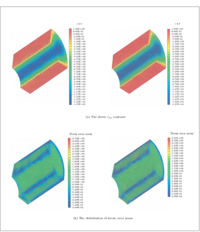
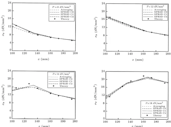
Figures 6 to 8 present the results of data transfer between two dierent meshes, using the 3D SPR method, based on C0, C1and C2continuity at P = 18 N/mm2. As obtained from the results, the maximum value of stress error norm occurs in the radius of 169 mm for P = 18 N/mm2. A good agreement can be observed between `coarse' and `ne' meshes in the contours of stress xy and stress error norm, before and after the transferring of state and internal variables. In Figure 9, the variations of stress, , with the radius of the cylinder are plotted at four various load steps of internal pressure, i.e. P = 8, 12, 14 and 18 N/mm2. The results are obtained by using the averaging method and 3D SPR technique, based on C0, C1 and C2 continuity, and compared with the theoretical solution given in [27]. A good
Figure 5. One-quarter of a circular tube subjected to the internal pressure, geometry, boundary conditions and material properties.
Figure 6. A circular tube; mapping of variables between two dierent meshes using 3D SPR method with C0 continuity
at P = 18 N/mm2.
agreement can be seen between the numerical and analytical results. Variations of the relative energy norm error with the element size are presented in Figure 10, at various load steps of internal pressure. The results demonstrate that the SPR technique based on C1 continuity creates a remarkable improvement in the accuracy of the proposed 3D algorithm. Also,
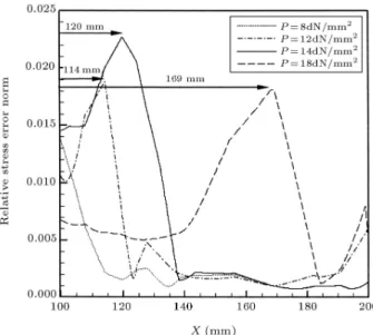
plotted in Figure 11 are variations of the relative stress error norm with the average element size at dierent internal pressures. A remarkable improvement in accuracy can be seen again for the SPR technique using C1 continuity. In Figure 12, the variation of relative stress error norm is presented with the radius of the cylinder at various load steps. This gure presents
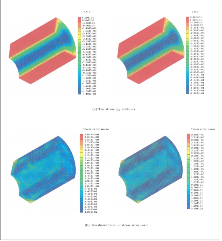
Figure 7. A circular tube; mapping of variables between two dierent meshes using 3D SPR method with C1 continuity
at P = 18 N/mm2.
the location of the maximum relative stress error norm at dierent internal pressures. It can be seen from the graph that the position of maximum error changes from the interior boundary of the cylinder at P = 8 N/mm2 to the exterior boundary at P = 18 N/mm2. Obviously, the results are identical with the maximum values of stress presented in Figure 9. These results
can be used in an automatic adaptive mesh generator to optimize the mesh at each load step.
CONCLUSION
In the present paper, the SPR method was rstly ex-tended to three-dimensional plasticity problems, based
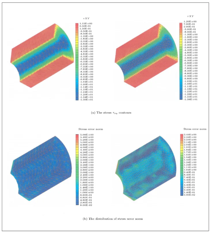
Figure 8. A circular tube; mapping of variables between two dierent meshes using 3D SPR method with C2 continuity
at P = 18 N/mm2.
on C0, C1 and C2 continuity. The technique was then employed to transfer the variables from the old mesh to the new one. The procedure of data transfer was performed in three dierent stages by transferring the internal variables from old Gauss points to old nodal points, mapping of variables from nodal points to new nodal points and, nally, transferring the new nodal
points to the new Gauss points. The eects of each variant of C0, C1 and C2 continuity were investigated using the relevant estimated error. It is shown how the new algorithm of the 3D SPR technique can be applied to accurately recover the stresses. Finally, a circular tube subjected to internal pressure was ana-lyzed numerically in order to illustrate the performance
Figure 9. A comparison between numerical and theoretical results for a circular tube; the variations of stress with
radius at four various load steps of internal pressure; P = 8, 12, 14 and 18 N/mm2.
Figure 10. A circular tube; the variations of relative energy norm error with element size at four various load steps of internal pressure; P = 8, 12, 14 and 18 N/mm2.
Figure 11. A circular tube; the variations of relative stress error norm with average element size at four various load steps of internal pressure; P = 8, 12, 14 and 18 N/mm2.
Figure 12. The variation of relative stress error norm with radius of cylinder at various load steps.
of the 3D SPR method in nonlinear problems using tetrahedral meshes. A good agreement was achieved between the numerical and analytical results. The results demonstrated that the SPR technique based
on C1 continuity gives a remarkable improvement in accuracy of the proposed 3D algorithm. In a later work, it will be shown how the proposed data transfer operators can be used in a three-dimensional automatic adaptive mesh generator to optimize the mesh at each load step.
REFERENCES
1. Zienkiewicz, O.C. and Zhu, J.Z. \The superconver-gence patch recovery and a posteriori error estimates. Part I: The recovery techniques", Int. J. Numer. Meth. Eng., 33, pp 1331-1364 (1992).
2. Zienkiewicz, O.C. and Zhu, J.Z. \The superconver-gence patch recovery and a posteriori error estimates. Part II: Error estimates and adaptivity", Int. J. Nu-mer. Meth. Eng., 33, pp 1365-1380 (1992).
3. Zienkiewicz, O.C., Boroomand, B. and Zhu, J.Z. \Re-covery procedures in error estimation and adaptivity. Part I: Adaptivity in linear problems", Comput. Meth. Appl. Mech. Eng., 176, pp 111-115 (1999).
4. Boroomand, B. and Zienkiewicz, O.C. \Recovery pro-cedures in error estimation and adaptivity. Part II: Adaptivity in nonlinear problems of elasto-plasticity behavior", Comput. Meth. Appl. Mech. Eng., 176, pp 127-146 (1999).
5. Gu, H. and Kitanmra, M. \A modied recovery proce-dure to improve the accuracy of stress at central area of bilinear quadrilateral element", J. Soc. Naval. Arch. Jpn., 188, pp 489-496 (2000).
6. Kitanmra, M., Gu, H. and Nobukawa, H. \A study of applying the superconvergent patch recovery method in large deformation problem", J. Soc. Naval. Arch. Jpn., 187, pp 208-210 (2000).
7. Babuska, I. and Rheinboldt, W.C. \A-posteriori error estimates for nite element method", Int. J. Numer. Meth. Eng., 12, pp 1597-1615 (1978).
8. Bank, R.E. and Weiser, A. \A-posteriori error esti-mator for elliptic partial dierential equations", Math. Comput., 44, pp 283-301 (1985).
9. Babuska, I., Zienkiewicz, O.C., Gago, J. and de Oliveira, E.R., Accuracy Estimates and Adaptive Re-nements in Finite Element Computations, John-Wiley (1986).
10. Zienkiewicz, O.C. and Taylor, R.L., The Finite Ele-ment Method, 1, McGraw-Hill (2000).
11. Johnson, C. and Hansbo, P. \Adaptive nite element methods in computational mechanics", Comput. Meth. Appl. Mech. Eng., 101, pp 143-181 (1992).
12. Ladeveze, E., Cognal, G., Pelle, J.P. \Accuracy of elastoplastic and dynamic analysis", Accuracy Esti-mates and Adaptive Renements in Finite Element Computations, I. Babuska, et al., Eds., John-Wiley, pp 181-203 (1986).
13. Samuelsson, A. and Wiberg, N.E. \Finite element adaptivity in dynamics and elastoplasticity", The Fi-nite Element Method in the 1990's, E. Onate et al., Eds., Springer-Verlag, pp 152-162 (1991).
14. Lee, N.S. and Bathe, K.J. \Error indicators and adaptive remeshing in large deformation nite element analysis", Finite Elem. Anal. Des., 16, pp 99-139 (1994).
15. Babuska, I. and Strouboulis, T. \Validation of a posteriori error estimators by numerical approach", Int. J. Numer. Meth. Eng., 37, pp 1073-1124 (1994). 16. Gu, H., Zong, Z. and Hung, K.C. \A modied
super-convergent patch recovery method and its application to large deformation problems", Finite Elem. Anal. Des., 40, pp 665-687 (2004).
17. Tang, X. and Sato, T. \Adaptive mesh renement and error estimate for 3D seismic analysis of liqueable soil
considering large deformation", J. Natural Disaster Science, 26, pp 37-48 (2004).
18. Ortiz, M. and Quigley, I.V. JJ. \Adaptive mesh renement in strain localization problems", Comput. Meth. Appl. Mech. Eng., 90, pp 781-804 (1991). 19. Camacho, G.T. and Ortiz, M. \Computational
mod-eling of impact damage in brittle materials", Int. J. Solids. Struct., 33, pp 2899-2938 (1996).
20. Camacho, G.T. and Ortiz, M. \Adaptive Lagrangian modeling of ballistic penetration of metallic targets", Comput. Meth. Appl. Mech. Eng., 142, pp 269-301 (1997).
21. Peric, D., Hochard, C., Dutko, M. and Owen, D.R.J. \Transfer operators for evolving meshes in small strain elasto-plasticity", Comput. Meth. Appl. Mech. Eng., 137, pp 331-344 (1996).
22. Khoei, A.R., Tabarraie, A.R. and Gharehbaghi, S.A. \H-adaptive mesh renement for shear band localiza-tion in elasto-plasticity Cosserat continuum", Com-mun. Nonl. Sci. Numer. Simul., 10, pp 253-286 (2005). 23. Khoei, A.R., Gharehbaghi, S.A., Tabarraie, A.R. and Riahi, A. \Error estimation, adaptivity and data transfer in enriched plasticity continua to analysis of shear band localization", Appl. Math. Model., pp 983-1000 (2007).
24. Zlamal, M. \Superconvergence and reduced integration in the nite element method", Math. Comput., 32, pp 663-685 (1978).
25. Babuska, I., Strouboulis, T. and Upadhyay, C.S. \A model study of the quality of a posteriori error esti-mator for linear elliptic problems. Error estimation in the interior of patchwise uniform grids of triangular", Comput. Meth. Appl. Mech. Eng., 114, pp 307-378 (1994).
26. Babuska, I., Strouboulis, T., Upadhyay, C.S. and Gan-garaj, S.K. \Computer-based proof of the existence of superconvergence points in the nite element method. Superconvergence of the derivatives in nite element solution of Laplace, Poisson and elasticity equations", Numer Meth for PDEs, 12, pp 347-392 (1996). 27. Owen, D.R.J. and Hinton, E., Finite Elements in
Plas-ticity: Theory and Practice, Pineridge Press, Swansea (1980).