Case–Control Study
Mark A. Kaelin
Department of Health Professions
Montclair State University
Upper Montclair, New Jersey
and
Manuel Bayona
Department of Epidemiology
University of North Texas
Contents
Lesson Plan . . . .
3
Glossary . . . .
6
Notes for Teachers . . . .
9
Teacher’s Narrative . . . .
16
Transparencies . . . .
30
Worksheet A: Case–Control Studies and Odds Ratio . . . .
40
Worksheet B: Case–Control Studies and Odds Ratio . . . .
43
Assessment (Student Version) . . . .
47
Assessment (Teacher’s Answer Key) . . . .
50
Optional In-Class Exercise (Student Version) . . . .
54
In-Class Exercise (Teacher’s Answer Key) . . . .
59
Copyright © 2004 by College Entrance Examination Board. All rights reserved.
College Board, SAT and the acorn logo are registered trademarks of the College
Entrance Examination Board. Other products and services may be trademarks of
their respective owners. Visit College Board on the Web: www.collegeboard.com.
Lesson Plan
TITLE: Case–Control Study
SUBJECT AREA: Biology, mathematics, statistics, environmental and health sciences
GOAL: To appreciate the value and limitations of the case–control study design
OBJECTIVES:
1. Introduce students to the principles and methods for designing and interpreting the results of a case–control study
3. Apply descriptive and analytical techniques in epidemiology, including the calculation and interpretation of the odds and the odds ratio
4. Understand the differences and the strengths and limitations of case–control studies as compared to other epidemiologic research designs
5. Identify the circumstances in which a case–control study would be an appropriate study design to test a hypothesis
TIME FRAME: Three 60-minute classes, with 2 hours of work outside class and including the optional in-class exercise
PREREQUISITE KNOWLEDGE: Basic knowledge of the cohort study design (see cohort study module), the 2 2 table, risk and relative risk
MATERIALS NEEDED: Copies of article, Worksheets A and B, and a hand calculator
PROCEDURE: The instructional unit has nine different sections:
1. Notes for teachers: Notes with basic concepts and procedures related to case–control studies and the calculation, interpretation and use of the odds ratio as a measure of association.
2. Teacher’s narrative: The teacher’s step-by-step instructions for teaching the module. Includes assigned reading—an article assigned for homework after Class 2 (Shands KN, Schmid GP, Dan BB, et al. Toxic-shock syndrome in menstruating women: association with tampon use and Staphylococcus aureus and clinical features in 52 cases. New England Journal of Medicine. 1980;303:1436–1442).
3. Transparencies: Transparencies that accompany Classes 1 and 2. 4. Worksheet A: In-class questions that accompany Class 1. 5. Worksheet B: In-class questions that accompany Class 2.
6. Assessment: Questions can be used as a quiz, homework assignment or in-class exercise to assess students’ understanding.
7. Assessment key: Suggested answers to assessment questions. 8. In-class exercise.
9. In-class exercise: Suggested answers to in-class exercise.
Recommended References
Friis RH, Sellers TA. Epidemiology for Public Health Practice.Gaithersburg, MD: Aspen Publishers: 1996.
Kelsey LJ, et al. Methods in Observational Epidemiology.2nd ed. Monographs in Epidemiology and Biostatistics. New York: Oxford University Press; 1996.
Lilienfeld DE, Stolley PD. Foundations of Epidemiology.3rd ed. New York: Oxford University Press; 1994. Mausner JS, Kramer S. Epidemiology—An Introductory Text.Philadelphia: WB Saunders; 1985.
NATIONAL SCIENCE EDUCATION STANDARDS: Science As Inquiry
• Abilities necessary to do scientific inquiry • Understanding of scientific inquiry
Science in Personal and Social Perspectives
• Personal and community health • Natural and human-induced hazards
Unifying Concepts and Processes
• Systems, order and organization • Evidence, models and measurement
National Science Education Standards, Chapter 6, available at: http://www.nap.edu/html/6a.html
National Standards for School Health Education:
• Students will comprehend concepts related to health promotion and disease prevention. • Students will demonstrate the ability to access valid health information and
health-promoting products and services.
• Students will analyze the influence of culture, media, technology and other factors on health.
• Students will demonstrate the ability to use goal-setting and decision-making skills to enhance health.
The National Standards for School Health Education available at: http://www.ericfacility.net/ ericdigests/ed387483.html
Glossary
Case–control study An analytical epidemiologic study design in which individuals who have the disease under study, also called cases, are compared to individuals free of disease (controls) regarding past exposures. Exposure differences between cases and controls are helpful to find potential risk or protec-tive factors. The purpose is to determine if there are one or more fac-tors associated with the disease under study.
Contingency table
(2 x 2 table) A table commonly used to display results of epidemiologic studies to calculate measures of disease frequency and association from dichoto-mous categorical variables. A typical 2 x 2 table in epidemiologic stud-ies is as follows:
Cases Noncases
Exposed a b
Nonexposed c d
A 2 2 table is commonly used to calculate the odds ratio (OR =
((a/c)/(b/d)). In cohort studies but not case-control studies, it can also be used to calculate the relative risk (RR = (a/(a + b)/c/(c+ d)).
Incidence rate A calculation of disease frequency that measures the probability of developing a disease in a given period of time. It is calculated by divid-ing the number of new cases by the total number of people susceptible to the disease at the beginning of the study period. As with other rates, the result may be multiplied by a multiple of 10 to obtain a convenient number.
Odds In epidemiology, odds of an attribute can be defined as the result of dividing the proportion of individuals with an attribute by the propor-tion of individuals without the attribute in a populapropor-tion. Odds can be interpreted as the probability of occurrence of an event as compared to the probability of nonoccurrence of an event in a population.
Odds ratio A measure of association typically used to quantify the strength of asso-ciation between a potential risk or protective factor (exposure) and an outcome. The odds ratio (OR) is a measure of the relative magnitude of
the odds of exposure among individuals who have the disease (cases) and the odds of exposure among individuals who do not have the dis-ease (controls): OR = (a/c)/(b/d). From a typical 2 x 2 table:
Cases Noncases
Exposed a b
Nonexposed c d
Odds of exposure among cases: a/c
Odds of exposure among controls: b/d
Odds ratio = (a/c)/(b/d)
Hence, OR = 1 means that the odds of exposure among cases are the same as the odds among the controls. Thus there is no evident associ-ation between exposure and disease. An OR > 1 denotes larger odds of exposure among the cases than among the controls. Thus individu-als who have the disease (cases) have a higher odds of having been exposed in the past than individuals without the disease (controls). This situation illustrates a risk factor. With the same reasoning, an OR < 1 denotes smaller odds of exposure among individuals with the disease as compared to controls, suggesting that controls have a higher odds of having been exposed. Therefore, this situation illus-trates a protective factor.
Onset (disease onset) Beginning of the disease or condition under study.
Prevalence The prevalence is a proportion in which the numerator includes existing cases of a disease or condition, and the denominator includes the pop-ulation from which the cases of disease came. The result is often multi-plied by a multiple of 10 to obtain a convenient number.
Relative risk The relative risk (RR) is a measure of association between a disease or condition and a factor under study. It is calculated by dividing the inci-dence rate of those exposed to the factor by the inciinci-dence rate of those not exposed to the factor.
RR Incidence in the exposed Incidence in the nonexposed
RR cannot generally be calculated in a case-control study because the entire population has not been studied, so incidences are unkown. From a 2 x 2 table of a cohort study the relative risk could also be calculated as follows:
Cases Noncases
Exposed a b
Nonexposed c d
Incidence in the exposed: a/(a+ b)
Incidence in the nonexposed: c/(c + d)
The RR is a measure of the relative magnitude of the incidence in the exposed and the incidence in the nonexposed. RR = 1 means that the incidence in the exposed is the same as the incidence in the nonex-posed, and so there is no evident association between exposure and disease. RR > 1 denotes a larger incidence in the exposed than the non-exposed. Thus exposure to the factor seems to increase the probability of developing the disease. With the same reasoning, RR < 1 denotes a smaller incidence in the exposed as compared to the nonexposed. Thus exposure to the factor seems to decrease the probability of developing the disease.
RR Incidence in the exposed Incidence in the nonexposed
= = a /(a + b)
Notes for Teachers
Definition of a Case-Control Study
A case–control studyis an investigation that compares a group of people with a disease to a group of people without the disease. Like many research designs, it is used by epidemiologists to identify and assess factors that are associated with diseases or health conditions, with the ulti-mate goal of preventing such diseases.
A case–control study begins with a group of cases of a specific disease or condition. A group of people without that disease or condition is selected as control, or comparison, subjects. The investigator then seeks to compare cases and controls with respect to previous exposures to fac-tors of interest. Information about prior exposure may be obtained by a variety of methods, including self-administered questionnaires, interviews and medical examinations. Because in case–control studies, information about exposure is generally collected after the disease has already occurred, these studies are sometimes called retrospective studies.
Case–control studies start with the outcome and look backward for the exposure, unlike cohort studies, which start from the exposure and look forward for the outcome. For example, a
case–control study of asthma in high school students may identify a group of students who suffer from asthma and compare them to a control group of students without asthma in regard to factors such as presence of carpets in the house, presence of household pets and family history of asth-ma. If the odds of exposure to one of these factors are different in the cases and controls, then that factor is associated with asthma and may influence the occurrence of the disease.
Identification of Cases
To conduct a case–control study, we must start by identifying a group of people who have the disease in question, typically called cases. One may identify cases through hospital registries or clinic records listing all patients having a certain disease. We can also locate cases through local health department disease registries. Cases can also be found in a predefined group that includes medical records, such as high schools and some industrial plants, or in a prepaid health insur-ance group.
Identification of Controls
Once individuals with the disease under study (cases) are identified, individuals without the dis-ease (controls) should be identified. Selection of controls for case–control studies is one of the
most difficult design issues in epidemiology because the apparent difference in prior exposure of cases and controls may be thought to be the result of the factors that cause the disease but may actually be the result of the process used to select the controls (an error called selection bias). Controls should be representative of the source population from which cases were derived. Although challenging and often expensive, the surest approach is to draw a random sample of controls from the source population from which the cases came.
Other sources of control groups include special groups such as friends, neighbors or relatives of the cases. Hospital- or clinic-based controls are frequently used but often are not representative of the source population. This happens when the reasons for attending the hospital or clinic may be different for cases and controls. For example, in a case–control study investigating the social and economic factors associated with depression, a certain clinic may be known to have the best physicians specializing in depression in a region. However, physicians with other specialties at the clinic may be no better than their peers in that region. If this is so, and cases and con-trols are both selected from that clinic, cases of depression may be representative of the whole region, whereas the controls represent only the local neighborhood, which may have different social and economic characteristics.
Analysis of the Data
Once the person planning a case–control study has identified the outcome of interest (disease or health condition) and the factors to be studied, a method for collecting information (e.g., a self-administered questionnaire, an interview form or a medical examination form) is developed. Data should include information about the outcome of interest (e.g., presence or absence of asthma) and the factors under study (e.g., presence or absence of carpeting, presence or absence of household pets and presence or absence of a family history of asthma).
Data analysis involves calculating the odds ratio as a measure of association between the dis-ease and each of the factors of interest. The odds ratio can be used to determine if there is an association and to quantify the magnitude of such an association.
Definition of an Odds Ratio
The odds ratio (OR), sometimes called the relative odds, is a measure of association between exposures and the disease or outcome. It is frequently used in case–control studies, in which incidence rates cannot be calculated. The odds ratio contrasts the odds of exposure among cases with the odds of exposure among controls.
Calculating the Odds Ratio
In a case–control study, investigators try to identify and assess factors that may influence the probability of developing the disease. A case–control study of the relationship between smoking and lung cancer may be analyzed by using a 2 2 table as follows:
Typical 2
2 Table for a Case–Control Study
Individuals With Individuals Without Lung Cancer Lung Cancer
(Cases) (Controls)
Smokers a b
Nonsmokers c d
Total a + c b + d
Hence, adenotes persons with lung cancer (cases) who smoked, bdenotes controls who smoked,
cdenotes persons with lung cancer (cases) who did not smoke, and ddenotes controls who did not smoke. The first column lists the total number of persons with lung cancer (a+ c) and the second column lists the total number of controls (b + d).
The odds ratio contrasts the odds of exposure (smoking) among the cases (individuals with lung cancer) with the odds of exposure (smoking) among the controls (individuals without lung cancer). The odds of exposure among the cases is the ratio of cases with exposure to cases without exposure (a/c). The odds of exposure among the controls is the ratio of controls who are exposed to controls who are not exposed (b/d).
Therefore the odds ratio is calculated as follows:
OR = (a/c)/(b/d) = ad/bc
Interpreting the Odds Ratio
A hypothetical case–control study in which 200 cases of lung cancer were compared to 200 con-trols regarding their smoking habits showed the following findings:
2
2 Table for a Case–Control Study of Lung Cancer and Smoking
Individuals With Individuals Without Lung Cancer Lung Cancer
(Cases) (Controls) Smokers 127 (a) (b) 35
Nonsmokers 73 (c) (d) 165
Total 200 200
Odds of exposure among cases: a/c = 127/73 = 1.7397 Odds of exposure among controls: b/d= 35/165 = 0.2121
Odds ratio = 1.7397/0.2121 = 8.2
The odds of exposure to smoking among cases of lung cancer are 8.2 times as large as the odds of smoking among controls. Therefore, the odds of smoking among individuals with lung cancer (cases) were 8.2 times as great as the odds among the controls, a magnitude that indicates an important association between lung cancer and smoking. Smoking could thus be a factor that increases the probability of having lung cancer.
Factors that increase the probability of having the disease are called risk factors.However, we cannot calculate an incidence rate of a disease based on a case–control study. This is because we do not know the size of the population from which the cases were drawn. The number of people exposed (a + b) and the number of people unexposed (c + d) are the arbi-trary results of the number of cases and controls that were selected and not representative of any real population. Therefore, we cannot calculate the risk of a disease in the exposed and unexposed.
As stated above, we can identify risk factors by calculating the odds of exposure among the cases and the controls and comparing them by calculating an odds ratio. It is important to real-ize that when this is done, we are comparing the odds in favor of exposure among the cases and controls [(a/c) / (b/d)]. Conceptually this is very different from comparing the odds in favor of disease among the exposed and unexposed [(a/b) / (c/d)], which is what we are really interested in being able to calculate.
Fortunately, however, algebraically the odds in favor of exposure among the cases and controls [(a/c) / (b/d)] are equal to ad/bc. And one can see that the odds in favor of disease among the exposed and unexposed [(a/b) / (c/d)] are also equal to ad/bc. Therefore, the odds in favor of exposure among the cases and controls are equal to the odds in favor of disease among the exposed and unexposed, which is what we really wish to calculate.
2
2 Table for a Case–Control Study of Lung Cancer and Smoking
Individuals With Individuals Without Lung Cancer Lung Cancer
(Cases) (Controls) Smokers 127 (a) (b) 35
Nonsmokers 73 (c) (d) 165
Total 200 200
Odds of exposure among cases: a/c = 127/73 = 1.7397 Odds of exposure among controls: b/d= 35/165 = 0.2121
Odds ratio = 1.7397/0.2121 = 8.2
The odds of exposure to smoking among cases of lung cancer are 8.2 times as large as the odds of smoking among controls. Therefore, the odds of smoking among individuals with lung cancer (cases) were 8.2 times greater than the odds among the controls, a magnitude that indicates an important association between lung cancer and smoking. Smoking could thus be a factor that increases the probability of having lung cancer.
Factors that increase the probability of having the disease are called risk factors.However, we cannot calculate an incidence rate of a disease based on a case–control study. This is because we do not know the size of the population from which the cases were drawn. The number of people exposed (a + b) and the number of people unexposed (c + d) are the arbi-trary results of the number of cases and controls that were selected and not representative of any real population. Therefore, we cannot calculate the risk of a disease in the exposed and unexposed.
As stated above, we can identify risk factors by calculating the odds of exposure among the cases and the controls and comparing them by calculating an odds ratio. It is important to real-ize that when this is done, we are comparing the odds in favor of exposure among the cases and controls [(a/c) / (b/d)]. Conceptually this is very different from comparing the odds in favor of disease among the exposed and unexposed [(a/b) / (c/d)], which is what we are really interested in being able to calculate.
Fortunately, however, algebraically the odds in favor of exposure among the cases and controls [(a/c) / (b/d)] are equal to ad/bc. And one can see that the odds in favor of disease among the exposed and unexposed [(a/b) / (c/d)] are also equal to ad/bc. Therefore, the odds in favor of exposure among the cases and controls are equal to the odds in favor of disease among the exposed and unexposed, which is what we really wish to calculate.
Sometimes the factor under study can decrease the probability of having the disease. Such fac-tors are called protective factors. Their association can also be measured with an odds ratio. For example, consider a hypothetical case–control study in which 250 obese individuals (cases) were compared to 250 nonobese individuals (controls) regarding the consumption of vegetables in their diets. The results showed the following:
2
2 Table for a Case–Control Study of Obesity
and Regularly Eating Vegetables
Obese Nonobese Individuals Individuals
(Cases) (Controls) Eat Vegetables 121 (a) (b) 171
Do Not Eat 129 (c) (d) 79
Vegetables
Total 250 250
Odds of exposure among cases: a/c= 121/129 = 0.9380 Odds of exposure among controls: b/d= 171/79 = 2.1646
Odds ratio = 0.9380/2.1646 = 0.43
The odds of exposure to eating vegetables among cases were 0.43 times as large as the odds of that exposure among controls. Therefore, the odds of exposure to eating vegetables among cases were 57% smaller than the odds of that exposure among controls. The results of this study show that eating vegetables was less likely to be found among cases than among controls. Eating veg-etables thus could be a protective factor decreasing the probability of being obese. Hence, the odds ratio can also measure how much smaller the odds of exposure are among cases as com-pared to controls.
Sometimes during a study no association is found between the study factor and the disease. This situation can also be measured with the odds ratio. Consider the results of a hypothetical case–control study in which 220 individuals suffering from depression (cases) were compared to 220 individuals not suffering from depression (controls) regarding the consumption of veg-etables in their diets:
2
2 Table for a Case–Control Study of Depression
and Eating Vegetables
Individuals With Individuals Without Depression Depression
(Cases) (Controls) Eat Vegetables 90 (a) (b) 90
Do Not Eat 130 (c) (d) 130
Vegetables
Total 220 220
Odds of exposure among cases: a/c = 90/130 = 0.6923 Odds of exposure among controls: b/d = 90/130 = 0.6923
Odds ratio = 0.6923/0.6923 = 1.0
The odds of exposure to eating vegetables among the individuals with depression (cases) are the same as the odds of exposure among controls. The odds ratio thus was found to be equal to 1.0, denoting a lack of association between the outcome (depression) and eating vegetables. The results of this study do not show an association between eating vegetables and having depression. Therefore an OR > 1 suggests a possible risk factor, an OR < 1 suggests a possible protective factor and an OR = 1 suggests no association.
Strengths of the Case–Control Study
Case–control studies have several advantages. They can be used to study infrequent (rare) dis-eases and are relatively inexpensive because no follow-up is necessary. Exposure is then ascer-tained retrospectively. The investigator does not have to wait for the accumulation of enough individuals who are developing the disease, as in cohort studies. For the same reason, case– control studies are particularly useful for studying diseases with long incubation or latency peri-ods. Because they are small and retrospective, they are often cheaper to do than cohort stud-ies and randomized controlled trials.
Limitations of the Case–Control Study
Unlike cohort studies, case–control studies cannot be used to compute incidence rates. Without knowing incidence, it is not possible to compute the relative risk. One can, however, use
case–control studies to compute the odds ratio, a measure of association that under certain con-ditions approximates the relative risk. (These concon-ditions will be explored later in the module.) The chronologic order of the exposure and disease, which is easy to elucidate in cohort studies, may be uncertain from the results of a case–control study because it may not be possible to know if the exposure occurred before the disease. For example, if a case–control study of asthma in high school students demonstrates an association with cat ownership, it may be difficult to know what happened first: the presence of cats or the first asthma attack. One can often over-come this problem by including only newly diagnosed cases.
In practice, case–control studies are often affected by selection bias. Selection bias may be pres-ent if the control group does not come from the same population as the cases. For example, if cases of asthma are drawn from a population of high school students, and controls without asth-ma are drawn from a population of older individuals who do not attend high school, one risks introducing a serious bias. This represents a problem because the factors related to asthma are different in young and older individuals. Consequently, many factors that might be found to be associated with asthma, based on a study of such mismatched cases and controls, might result merely from the fact that these two populations are of different age.
Information bias is another common problem of case–control studies. A type of information bias frequently found in case–control studies is recall bias. Recall bias may arise when individuals with a disease (cases) remember past exposures more completely (or less completely) than con-trols. This often happens because sick individuals try to figure out what caused their disease. Therefore, when they are interviewed they often remember more events from their past. In con-trast, individuals without disease (controls) have no special reason to remember past exposures. Although case–control studies are good for studying rare diseases, they are not generally good for studying rare exposures. For example, if we want to study the risk of asthma from working in a nuclear submarine shipyard, we would probably not do a case–control study because a very small proportion of people with asthma would have been exposed to such a factor.
Case–control studies cannot be used to study multiple diseases or conditions because it is neces-sary to guarantee that the control group is comparable for each disease or condition selected. Therefore, if one wants to study more than one disease, new groups of cases and controls are needed.
Teacher’s Narrative
Class 1
As Mr. Wilson monitored the 3–5 p.m., after-school, make-up-homework hall, he observed that many of the 20 students who were there seemed exhausted. Only a few of the students were working on making up their homework, in spite of the fact that when their homework was com-pleted, they could leave. Mr. Wilson also noticed what seemed to him like an abundance of cell phones on students’ desks and belts. When Mr. Wilson asked how many students had cell phones, 15 students raised their hands. Mr. Wilson wondered if the reason why so many of these students had not done their homework was because they spent too much time talking on their cell phones. Mr. Wilson, who is a history teacher, was behaving like a scientist, in particular like an epidemi-ologist. He was observing a group of people, counting the exposures and outcomes that people experience as they go about their daily lives, and hypothesizing: Talking too much on a cell phone causes students not to do their homework.
Epidemiologists have a tool for displaying the results of their studies, called a contingency table.The most basic contingency table is called a 22 tablebecause it has two rows and two columns. The two rows are for identifying the people who were and were not exposed to the hypothesized cause of the outcome, and the two columns are for identifying the people who have and do not have the outcome. (Transparency 1)
Outcome No Outcome
Exposed a b
Not Exposed c d
Total
Notice that four cells are formed where the two rows and two columns cross. Cell ais for people who were exposed (used cell phones) and had the outcome (did not do homework), cell bis for people who were exposed (used cell phones) and did not have the outcome (did homework), cell
cis for people who were not exposed (did not use cell phones) and had the outcome (did not do homework), and cell dis for people who were not exposed (did not use cell phones) and did not have the outcome (did homework).
Give students the case–control study Worksheet A and ask them to begin to answer Question 1 by labeling the 2 x 2 table to test Mr. Wilson’s hypothesis: Talking too much on a cell phone causes
students not to do their homework. Ask students what the outcome is (did not do homework) and what the exposure is (having a cell phone). (Transparency 2)
Did Not Do Did Homework Homework Had Cell Phone a b
Did Not Have c d
Cell Phone Total
Ask students to continue to answer Question 1 by placing Mr. Wilson’s counts into the 2 x 2 table. (Transparency 3)
Did Not Do Did Homework Homework Had Cell Phone 15 a b
Did Not Have 5 c d
Cell Phone
Total 20
Ask students which of the following inferences can be made based on the above data: A: 15 of 20 students who did not do their homework had cell phones. B: 15 of 20 students who had cell phones did not do their homework.
Probe until students uncover that based on Mr. Wilson’s sample only inference A can be made. Mr. Wilson began with a sample of students who had not done their homework and then inquired about whether or not they had a cell phone.
Inference B is in the form of an incidence rate (the rate at which new events occur in a popula-tion) or a risk (the proportion of people in a population who develop a new event by a certain time). For inference B to be made, Mr. Wilson would have had to begin with a sample of stu-dents who had cell phones and then determine whether or not they did their homework. You cannot calculate an incidence rate or a risk when you begin your inquiry with events (out-comes) that have already occurred and then collect data about the hypothesized cause (exposure). So how do epidemiologists numerically express the degree to which an exposure and outcome tend to turn up together, in a study that began with existing events? By calculating the oddsof having had an exposure among a sample that already has the outcome. The odds are the ratio of the number of times one alternative occurs to the number of times the other alternative occurs.
Ask students to answer Question 2 by calculating what the odds of having had a cell phone were among Mr. Wilson’s sample of students who had not done their homework. (15 to 5 or 3 to 1) Ask students if the odds of 3 to 1 support Mr. Wilson’s hypothesis: Talking too much on a cell phone causes students not to do their homework.
Probe until students uncover that it depends on what the odds of cell phone use were among a group of students who had done their homework. If necessary, refer students back to
Transparency 3.
Knowing that the students who were practicing for the spring concert would not have been able to practice if they had not done their homework, Mr. Wilson walked down the hall to the room in which the school orchestra was practicing and asked the 40 students who were practicing
whether or not they had cell phones. Thirty students raised their hands.
Ask students to continue to answer Question 1 by placing these counts in Mr. Wilson’s 2 x 2 table. (Transparency 4)
Did Not Do Did Homework Homework Had Cell Phone 15 a b30
Did Not Have 5 c d10
Cell Phone
Total 20 40
Ask students to answer Question 3 by calculating what the odds of having had a cell phone were among the students who had done their homework. (30 to 10 or 3 to 1)
Ask students whether this hypothesis would have been supported if the odds of cell phone use among a group of students who had done their homework were 3 to 1. (No, the odds are the same.)
Ask students if the counts presented in the 2 x 2 table below support Mr. Wilson’s hypothesis. (Yes) (Transparency 5)
Did Not Do Did Homework Homework Had Cell Phone 15 a b10
Did Not Have 5 c d30
Cell Phone
Ask students to answer Question 4 by calculating the odds of cell phone use among the group of students, depicted in Transparency 5, who had done their homework. (10 to 30 or 1 to 3) Ask students what mathematical computation would allow them to complete the following statement:
The odds of having a cell phone among the students who had not done their homework were _____ times as large as the odds of having a cell phone among the students who had done their homework.
(Divide the odds of cell phone use among the students who had not done their homework by the odds of cell phone use among the students who did do their homework.)
Ask students to answer Question 5 by completing the preceding statement based on the data presented in the 2 x 2 table above, depicted in Transparency 5. ((3/1)/(1/3) = 9)
Tell students that epidemiologists call what they have just calculated an odds ratio. An odds ratio is the ratio of two odds.
Ask students to answer Question 6 by describing what an odds ratio of 9 means. (The odds of having a cell phone among the students who had not done their homework were 9 times as large as the odds of having a cell phone among the students who had done their homework.)
Ask students to answer Question 7 by developing a formula for calculating an odds ratio using the letters of the four cells, a, b, cand d. ((a/c)/(b/d))
Ask students if the counts presented in the 2 x 2 table below support Mr. Wilson’s hypothesis. (Transparency 6) (No)
Did Not Do Did Homework Homework Had Cell Phone 15 a b35
Did Not Have 5 c d5
Cell Phone
Total 20 40
Ask students to answer Question 8 by calculating the odds of cell phone use among the group of students, depicted in Transparency 6, who had done their homework. (35 to 5 to 7 to 1) Ask students to answer Question 9 by calculating the odds ratio for the above data. ((3/1)/(7/1) = .43)
(The odds of having a cell phone among the students who had not done their homework were .43 times as large as the odds of having a cell phone among the students who had done their homework.)
Tell students that epidemiologists call this research design a case–control study. Ask students which of the following questions the case–control study answers
(Transparency 7)
A: What is the ratio of the odds of having the exposure among a group of people with the outcome to the odds of having the exposure among a group of people without the outcome?
B: What is the ratio of the odds of having the outcome among a group of people with the exposure to the odds of having the outcome among a group of people without the exposure?
Probe until students uncover that because the case–control study starts with people with and without the outcome and looks backward for exposure data, the case–control study answers Question A.
Keep in mind that epidemiology is “ . . . the study of the distribution and determinants of health-related states or events in specified populations and the application of this study to the control of health problems.”
Ask students, if they are interested in “the control of health problems,” to which of the above questions do they want an answer.
Probe until students uncover that if they are interested in the control of health problems, they really want an answer to Question B, not A, because health problems will be controlled by avoid-ing or eliminatavoid-ing the exposure and preventavoid-ing the outcome.
Although it may not seem to make sense intuitively, it can be shown algebraically that the case–control study also answers Question B.
Ask students to look at their answer to Question 7, in which they developed a formula for calcu-lating an odds ratio using the letters of the four cells, a, b, c,and d. The formula was (a/c)/(b/d). Note that this is the formula for the answer to Question A: What is the ratio of the odds of hav-ing the exposure among a group of people with the outcome to the odds of havhav-ing the exposure among a group of people without the outcome?
Ask students to solve the equation (a/c)/(b/d) = _____. (ad/cb)
Now ask students to answer Question 11 by developing a formula for calculating an odds ratio, using the letters of the four cells, a, b, c, and d, to answer Question B: What is the ratio of the odds of having had the outcome among a group of people with the exposure and
a group of people without the exposure? Have students assume that the control group is a representative sample of one out of every k people with popluation from which the cases were chosen. (The odds of having had the outcome among a group of people with the exposure are a/kb, and the odds of having had the outcome among a group of people without the exposure are c/kd, or (a/kb)/(c/kd)).
Ask students to solve the equation (a/kb)/(c/kd) = _____. (ad/cb)
Ask students to compare their formulas for answering Questions A and B. (They are algebraically the same.)
Tell students that not only does a case–control study tell us the odds of having had an exposure among groups of people with and without an outcome, but more important, it tells us what epi-demiologists really want to know, the odds of having had an outcome among groups of people with and without an exposure.
Point out to students that the odds of developing an outcome among a group of people with and without an exposure are not the same as the risk of developing an outcome among groups of people with and without an exposure. It is not possible, based on a case–control study, to calculate the risk of developing an outcome among groups of people with and without an exposure, and therefore it is not possible to calculate a relative risk.
However, under certain circumstances it is possible, based on a case–control study, to calculate a measure of association that will approximate the relative risk. Students will uncover these cir-cumstances in the next class.
Class 2
(At the end of this class, students should be able to explain the circumstances under which it is and is not possible to calculate a good approximation of the relative risk from a case–control study.) Tell students that we would like to measure the magnitude of the association between smoking and lung cancer in Smithtown, a town with approximately 400,000 inhabitants who are 18 years of age and older.
On the basis of a recent report from the National Health and Nutrition Examination Survey, we expect that approximately 25% of Smithtown’s population are smokers. And on the basis of a recent epidemiologic report, we expect that approximately 1 person in 1,000 will develop lung cancer per year (annual incidence) and that people live an average of 2.5 years after they devel-op lung cancer. The report indicated that the incidence of lung cancer in smokers was about five times as large as the incidence in nonsmokers (RR = 5.0) in Smithtown.
Ask students to use the data from the previous research report that are displayed in Table 1 to calculate the relative risk of lung cancer for cigarette smokers in the total population.
Compare students’ answers to the answer below and address misconceptions. RR = (250/100,000)/(150/300,000) = 0.0025/0.0005 = 5.0
Table 1. Total Adult Population of Smithtown
Lung Cancer
Present Absent Total Smokers 250 a b 99,750 100,000
Nonsmokers 150 c d 299,850 300,000
Total 400 399,600 400,000 Now ask students to use the data from the previous research report that are displayed in Table 1 to calculate the odds ratio for developing lung cancer for cigarette smokers.
Compare students’ answers to the answer below and address misconceptions. OR = (250/99,750)/(150/299,850) = 0.0025062/0.0005002 = 5.01
Please note that the relative risk of lung cancer for cigarette smokers and the odds ratio for developing lung cancer for cigarette smokers are almost identical.
Ask students why they think this is the case. Why, given the different formulas for the RR (a/a+ b)/(c/c + d) and the OR (a/b)/(c/d), are the RR and OR so similar?
Probe until students uncover the similarities in the two formulas when a disease is rare. When a disease is rare, a+ b(100,000) is almost equal to b(99,750), and c+ d(300,000) is almost equal to d(299,850).
Now tell students to assume that we want to see if the actual situation in Smithtown is similar to that expected based on the Center for Disease Control and Prevention (CDC) information displayed in Table 1. However, to study the entire population of 400,000 people would be very expensive and time-consuming. We would need to interview all residents to obtain information about their ciga-rette smoking and study their medical records to confirm whether or not they have lung cancer. Tell students to assume that we have the resources to interview and study a maximum of 800 individuals.
Ask students if it would be feasible to do a cohort study. Probe until students realize that a cohort study would not feasible because the anticipated incidence of lung cancer in Smithtown is only 1 per 1,000 population per year, and therefore a cohort study of 800 residents may not result in even 1 case of lung cancer in every year of follow-up.
Ask students if it would be feasible to do a case–control study. Probe until students realize that this would be feasible because the study could begin immediately with a total of 800 partici-pants that would consist of some combination of Smithtown’s residents with existing cases of lung cancer and a control group.
Tell students to assume that this case–control study would include all of Smithtown’s 400 resi-dents with lung cancer (cases) and a randomly selected control group of 400 resiresi-dents from the rest of the population (a typical case–control study).
Ask students to use the data displayed in Table 2 to calculate the odds ratio for having been a cig-arette smoker among those with lung cancer. Note that all 400 cases were included and that the proportion of smokers is 25% among controls (which is as close as one can get with whole numbers of people to the 24.96% proportion of smokers among those without lung cancer in Table 1).
Table 2. Case–Control Study (400 Cases and 400 Controls)
Lung Cancer
Present Absent Total Smokers 250 a b' 100 350
Nonsmokers 150 c d' 300 450
Total 400 400 800
Compare students’ answers to the answer below and address misconceptions. OR = (250/150)/(100/300) = 1.666/0.333 = 5.0
Remind students that they have been told that a relative risk cannot be directly calculated based on the results of a case–control study. We now want to examine why that is the case: It is because no incidence rates or risks are available. For the purpose of this example, let us introduce a concept that epidemiologists do not generally use (for reasons that will become apparent), the relative proportion, defined as the proportion of exposed people in a case– control study who are cases divided by the proportion of unexposed people in the same study who are cases. On the basis of data displayed in Table 2, calculate the relative proportion of lung cancer among the cigarette smokers and nonsmokers in this case–control study.
Compare students’ answers to the answer below and address misconceptions.
Relative proportion = (250 / 350) / (150 / 450) = 0.7142857 / 0.333 = 2.145 Point out to students that the odds ratio and the relative proportion are different and that the odds ratio is a good estimator of the relative risk in Smithtown’s total population shown in
Table 1. In contrast, the relative proportion is a poor estimator of the relative risk in Smithtown’s total population.
Ask students why the relative proportion is a poor estimator of the actual relative risk in Smithtown’s total population.
Probe until students realize that the calculation of the relative proportion is the ratio of two pro-portions (a/a + b’ and c/c + d’), neither of which represents the risk (or incidence rate) of lung cancer in a population. Both are artifacts of the proportion of cases and controls chosen for study. Therefore, the fact that the ratio of the two bears little relation to the relative risk is not surprising. This ratio is not a good estimator of the relative risk in the population because it is affected by our arbitrary decision to select 400 cases and 400 controls.
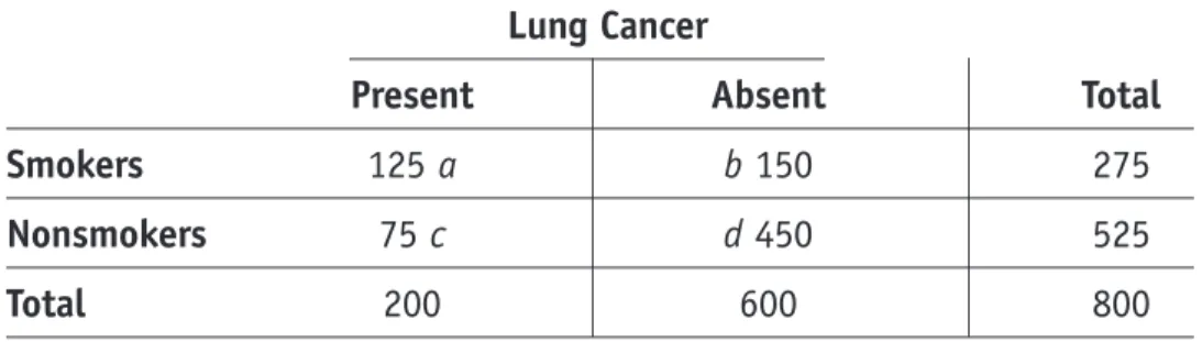
Tell students to assume that they had done another case–control study, and this time they included a random sample of 200 of Smithtown’s 400 residents with lung cancer (cases) and a randomly selected control group of 600 residents from the rest of the population, with the pro-portion of expected smokers (exposed) to be 25% as suggested by the CDC. The results would be as depicted in Table 3.
Table 3. Case–Control Study (200 Cases and 600 Controls)
Lung Cancer
Present Absent Total Smokers 125 a b 150 275
Nonsmokers 75 c d 450 525
Total 200 600 800
On the basis of the data displayed in Table 3, ask students to calculate the odds ratio for having been a cigarette smoker among those with lung cancer.
Compare students’ answers to the answer below and address misconceptions. OR = (125/75) / (150/450) = 1.666/0.333 = 5.0
Now ask students to calculate the relative proportion of lung cancer for cigarette smokers and nonsmokers, based on our arbitrary decision to select 200 cases and 600 controls.
Compare students’ answers to the answer below and address misconceptions.
Relative proportion = (125/275)/(75/525) = 0.454545/0.142857 = 3.182
Point out to students that the odds ratio and the relative proportion are again different, and that the odds ratio is still a good estimator of the relative risk in Smithtown’s total population
shown in Table 1. In contrast the relative proportion is a poor estimator of the relative risk in Smithtown’s total population. The ratio of disease proportions between exposed and nonexposed is now 3.182—not 2.145, as in the previous case–control design (Table 2)—and it is certainly not 5.0, as the relative risk is in the total population (Table 1). This again is because the rela-tive proportion is affected by the arbitrary decision to select 200 cases and 600 controls.
Emphasize to students that the odds ratio is a good estimator of the relative risk when the disease is rare and the cases and controls are representative of the ill and non-ill individuals in the total population, respectively. One cannot calculate the relative risk from a case–control study, as no incidence rates are available. And the relative proportion of cases among exposed and unexposed people in a case–control study is unreliable as an approximation of the relative risk, because it is an artifact of the relative size of the case and control groups, which in turn is the result of an arbitrary decision of the investigator. The relative proportion does not reliably estimate the relative risk in an actual population, so epidemiologists do not use the relative proportion.
In conclusion, ask students under what circumstances it is possible to estimate the relative risk from a case–control study.
Probe until students uncover that relative risk may be estimated from a case–control study when two criteria are met:
1. When the previous exposures of the cases and controls are representative of the previous exposures of the population from which they were selected (so the odds ratio from the case–control study is close to the odds ratio that one would have expected from a cohort study)
2. When the disease is rare (so the odds ratio is a close approximation of the relative risk) Ask students to answer Question 12 on their case–control study Worksheet B by reading an epi-demiologic description of a case–control study and drawing a diagram of the study design on a timeline. Tell students to be sure to depict when the
• Epidemiologist begins to observe the study participants
• Epidemiologist determines whether the participants were exposed or unexposed • Epidemiologist determines whether the participants have or do not have the outcome
Show students the following description of a case–control study. (Transparency 9)
“To examine the possible relation of an exposure to a certain disease, we identify a group of individuals with that disease (called cases) and, for purposes of comparison, a group of people without that disease (called controls). We determine what proportion of the cases were exposed and what proportion were not. We also determine what propor-tion of the controls were exposed and what proporpropor-tion were not.” (Leon Gordis,
Epidemiology, Philadelphia, WB Saunders, 2000, page 140) Compare students’ diagram to Transparency 10.
Tell students that selecting an appropriate control group has been called “ . . . one of the most difficult challenges in epidemiology” (Leon Gordis, Epidemiology, Philadelphia, WB Saunders, 2000, page 144).
Ask students why they think this is so. Probe until students uncover that in a case–control study, whether or not there is association between the exposure and the outcome will ultimately be determined by comparing the number of cases with and without the exposure to the number of controls with and without the exposure and calculating the odds and odds ratio.
Toxic shock syndrome is an uncommon but severe acute illness characterized by fever, low blood pressure, a widespread red rash and involvement of other body organs. It is a medical emergency that requires prompt treatment. When an epidemic of toxic shock syndrome began in the early 1980s, epidemiologists at the CDC carried out a case–control study to try to identify exposures that were associated with toxic shock syndrome. Among the exposures considered were tampons.
Ask students what would be an appropriate control group in a case–control study testing the hypothesis that use of tampons was associated with toxic shock syndrome. (Answer:
Menstruating women who do not have toxic shock syndrome) Ask students on what basis they concluded that this would be an appropriate control group.
Probe until students uncover that an appropriate control group would be made up of individuals who belong to the same population as the cases, who are free of the disease but who have the same opportunity as the cases to have had the exposure.
Ask students what would be an inappropriate control group in a case–control study testing the hypothesis that tampons cause toxic shock syndrome. (Answer: Men, nonmenstruating women) Emphasize that by selecting a particular control group one can unintentionally distort the pro-portion of controls that were exposed, and therefore the calculation of the odds ratio will be misleading.
Ask students to consider each of the following groups of cases and answer Question 13 by • Identifying an appropriate control group
• Identifying an inappropriate control group
• Assuming that there is really no association between exposure and outcome, explaining how the selection of an inappropriate control group would affect the odds ratio
Effect of Choosing Case Appropriate Inappropriate Inappropriate Group Control Group Control Group Control Group
a. Hypothesis: Inoculation with the measles, mumps and rubella vaccine causes autism. Children from a
particular town who had been diagnosed with autism.
b. Hypothesis: Hair dye causes breast cancer. All women
diag-nosed with breast cancer from a par-ticular hospital
c. Hypothesis: Body piercing causes hepatitis B. Students who went
to the nurse’s office with symptoms later diagnosed as those of hepatitis B.
d. Hypothesis: Being a member of a fraternity or sorority causes binge drinking. Students who had
been brought to a college infirmary and who were drunk.
e. Hypothesis: Playing violent video games causes violent behavior. Students who had
been expelled from high school for fighting.
f. Hypothesis: Having a cell phone causes students not to do their homework. Students who were
in an after-school,
For homework ask students to answer Question 14 on their case–control study Worksheet B by reading the article on toxic shock syndrome written by Katherine Shands and others, identifying the source of the control group and explaining the appropriateness of the control group.
(Shands KN, Schmid GP, Dan BB, et al. Toxic-shock syndrome in menstruating women: association with tampon use and Staphylococcus aureus and clinical features in 52 cases. New England
Journal of Medicine. 1980;303:1436–1442.)
Ask students to look at the diagram they drew to answer Question 12, and answer Questions 15–20. 15. Would the case–control study design be appropriate for testing a hypothesis for a disease
that is rare?
16. How accurate are the data about exposure in a case–control study? 17. Would the exposure data be more accurate for the cases or the controls?
18. How certain are you about the time order of the exposure and the outcome in a case–control study?
19. What would happen to the odds ratio of a case–control study if the controls who were selected did not have the same opportunity to come in contact with the exposure as the cases?
Transparency 1
Outcome No Outcome
Exposed a b
Not Exposed c d
Transparency 2
Did Not Do Did Homework Homework Had Cell Phone a b
Did Not Have c d
Cell Phone Total
Transparency 3
Did Not Do Did Homework Homework Had Cell Phone 15 a b
Did Not Have 5 c d
Cell Phone
Total 20
Which of the following inferences can be made based on the above data? A: 15 of 20 students who do not do their homework have cell phones. B: 15 of 20 students who have cell phones do not do their homework.
Transparency 4
Did Not Do Did Homework Homework Had Cell Phone 15 a b30
Did Not Have 5 c d10
Cell Phone
Transparency 5
Did Not Do Did Homework Homework Had Cell Phone 15 a b10
Did Not Have 5 c d30
Cell Phone
Total 20 40
Ask students what mathematical computation would allow them to complete the following statement:
The odds of having a cell phone was _____ times as large among students who had not done their homework compared to the students who did do their homework.
Transparency 6
Did Not Do Did Homework Homework Had Cell Phone 15 a b35
Did Not Have 5 c d 5
Cell Phone
Transparency 7
A What is the ratio of the odds of having the exposure among a group of people with the outcome to the odds of having the exposure among a group of people without the outcome?
B What is the ratio of the odds of having the outcome among a group of people with the exposure to the odds of having the outcome among a group of people without the exposure?
Transparency 8
Transparency 9
“To examine the possible relation of an exposure to a certain disease, we identify a group of individuals with that disease (called cases) and, for purposes of comparison, a group of people without that disease (called controls). We determine what proportion of the cases were exposed and what proportion were not. We also determine what proportion of the controls were exposed and what proportion were not.” (Leon Gordis, Epidemiology, Philadelphia, WB Saunders, 2000, page 140)
Transparency 10
E
E
E
E
DZ
DZ
Time
Name: __________________________ Date: _____/_____/_____
Worksheet A: Case–Control Studies
and Odds Ratios
1. Complete the 2 x 2 table.
a b
c d
2. Calculate the odds.
3. Calculate the odds.
5. Complete the following statement:
The odds of having a cell phone was _____ times as large among the students who had not done their homework compared to the students who did do their homework.
6. What does the odds ratio mean?
7. Create a formula.
9. Calculate the odds ratio.
10. What does the odds ratio mean?
Name: __________________________ Date: _____/_____/_____
Worksheet B: Case-Control Studies
and Odds Ratios
12. Draw a diagram.
13. Identify an appropriate control group, identify an inappropriate control group, and, assum-ing that there is really no association between exposure and outcome, explain how the selection of an inappropriate control group would affect the odds ratio.
Effect of Choosing Case Appropriate Inappropriate Inappropriate Group Control Group Control Group Control Group
a. Hypothesis: Inoculation with the measles, mumps and rubella vaccine causes autism. Children from a
particular town who had been diagnosed with autism.
b. Hypothesis: Hair dye causes breast cancer. All women
diag-nosed with breast cancer from a par-ticular hospital
c. Hypothesis: Body piercing causes hepatitis B. Students who went
to the nurse’s office with symptoms later diagnosed as those of hepatitis B.
d. Hypothesis: Being a member of a fraternity or sorority causes binge drinking. Students who had
been brought to a college infirmary and who were drunk.
e. Hypothesis: Playing violent video games causes violent behavior. Students who had
been expelled from high school for fighting.
f. Hypothesis: Having a cell phone causes students not to do their homework. Students who were
in an after-school, make-up-homework hall.
14. Identify the source of the control group and explain the appropriateness of the control group.
While looking at a diagram of a case–control study, answer the following questions. 15. Would the case–control study design be appropriate for testing a hypothesis for a disease
that is rare?
16. How accurate are the data about exposure in a case–control study?
18. How certain are you about the time order of the exposure and the outcome in a case– control study?
19. What would happen to the odds ratio of a case–control study if the controls who were selected did not have the same opportunity to come in contact with the exposure as the cases?
Assessment (Student Version)
(These questions can be used as a quiz, homework assignment or in-class exercise.) 1. Circle all of the statements below that are true regarding the case–control study design.
a. Permits direct estimation of disease risk (probability of developing the disease) and the relative risk.
b. Is a logical approach to the study of multiple outcomes. c. Is a logical approach to the study of multiple exposures.
d. Is a logical approach to the study of multiple outcomes and multiple exposures. e. Is frequently limited because of recall bias.
f. Is expensive because it is necessary to follow up study subjects in real time.
g. Uses the odds ratio as a measure of association between each exposure and the outcome. h. Starts with the selection of exposed and nonexposed individuals and compares their
inci-dence rates.
2. A hypothetical case–control study was conducted to identify exposures associated with a neurologic disorder in adolescents that is characterized by headaches and in a few severe cases seizures. Cases (persons with the neurologic disorder) were compared to a randomly selected control group of adolescents from the same schools the cases attended. The results of the study showed that the odds ratio for the disease, comparing those who played video games every day to those who did not play video games every day, was 2.1. The researchers also found that the odds ratio was 0.60, comparing those who regularly read books, other than school textbooks, to those who did not.
Circle all of the statements below that are true regarding this case–control study.
a. Cases (students with the neurologic disorder) had greater odds of having played video games than controls.
b. Adolescents who played video games every day had odds of having the neurologic disorder that were 2.1 times as large as the odds of those who did not play video games every day. c. Playing video games appeared to be a protective factor because it was associated with
reduced odds of having the neurologic disorder.
d. Reading regularly was associated with increased odds of having the neurologic disorder by 60%.
e. Reading regularly is not associated with the neurologic disorder because the odds ratio is under 1.0.
3. The use of cellular phones has been associated with the development of brain cancer, as evidenced in several studies. However, other studies have shown no such association. The table below includes the results of a case–control study of brain tumors and the regular use of cellular phones. This study was conducted using a control group made up of a random sample of the population of high school students who attended the same schools where the students with brain tumors were found.
Brain Tumors No Brain Tumors Cell Phones 63 185
No Cell Phones 96 292
Total
a. How many study subjects were cases? b. How many study subjects were controls? c. What was the ratio of controls to cases? d. What are the odds of exposure among cases? e. What are the odds of exposure among controls?
f. Calculate the odds ratio that compares exposure to cellular phones among those with and without the disease.
g. Calculate the odds ratio that compares disease among those who are exposed and those who are not exposed to cellular phones.
4. Leprosy, also called Hansen’s disease, is a disease produced by infection with a bacterium called Mycobacterium leprae. It has a long incubation period (time between getting infected and developing the disease), usually several years. Leprosy is a disease of low incidence in the United States; only 108 new cases were reported in 1999. If you are called to give advice on the type of study design to be conducted to assess the possible association between several exposures and leprosy, which design would you suggest and why? a. Case–control study
b. Cohort study
5. Following are the results of a study that used a case–control design. This study evaluated factors associated with admission to college. A total of 650 students were admitted to col-lege (cases), and they were compared to 650 students who were not admitted to colcol-lege (controls). The purpose of this study was to identify factors that are associated with the likelihood of being accepted into college.
Results of a Hypothetical Study of Factors Related
to Admission to College
Factor Odds Ratio
Female gender 1.4
Alcohol consumption 0.5
Sedentary life 1.0
Smoking 0.4
Illicit drug use 0.2
Regular sports practice 2.1
Circle all of the statements below that are true regarding this case–control study. a. Being female was associated with increased odds of being admitted into college. b. Females had 40% greater odds of being admitted into college as compared to males. c. Alcohol consumption was not associated with being admitted into college.
d. Those who had been admitted to college had half the odds of drinking alcohol as those who were not admitted to college.
e. Sedentary life was not associated with admission to college.
f. The odds of smoking were 60% lower in students admitted to college than among those who were not admitted to college.
g. The odds of admission to college were 20% lower in those who used illicit drugs than among those who did not use illicit drugs.
h. The odds of admission to college were 2.1 times as high among students who practiced sports regularly than among those who did not practice sports regularly.
Assessment (Teacher’s Answer Key)
(These questions can be used as a quiz, homework assignment, or in-class exercise.) 1. Circle all of the statements below that are true regarding the case–control study design.
a. Permits direct estimation of disease risk (probability of developing the disease) and the relative risk.
b. Is a logical approach to the study of multiple outcomes. c. Is a logical approach to the study of multiple exposures.
d. Is a logical approach to the study of multiple outcomes and multiple exposures. e. Is frequently limited because of recall bias.
f. Is expensive because it is necessary to follow up study subjects in real time.
g. Uses the odds ratio as a measure of association between each exposure and the outcome. h. Starts with the selection of exposed and nonexposed individuals and compares their
inci-dence rates.
2. A hypothetical case–control study was conducted to identify exposures associated with a neurologic disorder in adolescents that is characterized by headaches and in a few severe cases seizures. Cases (persons with the neurologic disorder) were compared to a randomly selected control group of adolescents from the same schools the cases attended. The results of the study showed that the odds ratio for the disease, comparing those who played video games every day to those who did not play video games every day, was 2.1. The researchers also found that the odds ratio was 0.60, comparing those who regularly read books, other than school textbooks, to those who did not.
Circle all of the statements below that are true regarding this case–control study.
a. Cases (students with the neurologic disorder) had greater odds of having played video games than controls.
b. Adolescents who played video games every day had odds of having the neurologic disorder that were 2.1 times as large as the odds of those who did not play video games every day. c. Playing video games appeared to be a protective factor because it was associated with
reduced odds of having the neurologic disorder.
d. Reading regularly was associated with increased odds of having the neurologic disorder by 60%.