Base year recalculation methodologies for structural changes

(1)

Base year recalculation methodologies for

structural changes

Appendix E to the GHG Protocol Corporate Accounting and

Reporting Standard Revised Edition

Version January 2005

Introduction

Making meaningful comparisons of emissions data over time is an integral part of any corporate GHG report that aims to be credible, transparent and useful to

stakeholders.

A prerequisite for such meaningful comparisons is a consistent data set over time, or in other words, comparisons of like with like over time. In order for this condition to be fulfilled, the inventory boundary must be held consistent between those data sets that are used for a direct comparison over time.

A base year is a reference point in the past with which current emissions can be compared. In order to maintain the consistency between data sets, base year emissions need to be recalculated when structural changes occur in the company that change the inventory boundary (such as acquisitions or divestments).

In practice this task is often more complicated than it appears on the face of it. This guidance document is an appendix to the GHG Protocol Corporate Standard

Revised Edition (March 2004), and clarifies some of the issues around base year

recalculations that often create confusion.

Firstly, this guidance document deals with GHG inventory recalculations under the so-called fixed base year approach, which is essentially a fixed historical reference with which to compare current emissions (see chapter 5 of the revised Corporate

Standard). Different options for making recalculations are presented, and it is argued

that under the fixed base year approach, the overall comparison over time is not affected by the choice of option, while one option is more practicable than the other. The second part of this document describes the application of the different options identified in the previous section under the so-called rolling base year approach (see step 4 of chapter 11 of the revised Corporate Standard ( Setting GHG targets ). It investigates the implications of different methods and concludes that the choice of method can have a bearing on which emission sources are included or excluded from the overall emissions comparison over time.

Thus, it will be important to transparently document the choice of method when a rolling base year is used, especially as this can be relevant for the compliance with a corporate target.

(2)

Base year recalculation methodologies for structural changes Please send your comments and questions to Simon Schmitz at [email protected]

1 Base year recalculation methodologies for structural changes

using a fixed base year

Chapter 5 ( Tracking emissions over time ) of the revised Corporate Standard describes how to establish a fixed base year and recalculate the emissions from that year in case of structural changes.

After recalculations under the fixed base year approach, emissions sources from an acquired company are included both with their emissions in the base year (when the acquiring company didn t control these sources yet) and in the current years. Similarly, emission sources from divested facilities/companies are excluded both with their emissions in the base year (when they were still controlled by the divesting company) and the current years.

As recommended in chapter 5, emissions should be recalculated for the entire year ( all-year option), rather than only for the remainder of the reporting period after the structural change occurred (the pro-rata option). The all-year option avoids having to recalculate base year emissions again in the succeeding year.

This can be described as the all-year option, since the inventory includes emissions from all facilities from January to December at all times.

In contrast, the pro-rata option operates on a step-by-step basis. After making the first recalculation, the inventory excludes a portion of the acquired or divested facility in at least the base and current year s inventories, until the full recalculation is made in the following year.

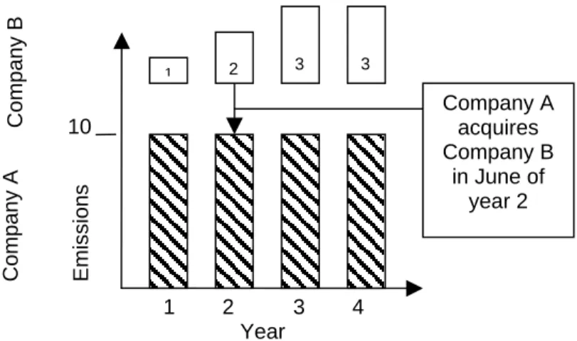
To illustrate, Figure 1 describes example Z: the acquisition by a company A of a company B in the middle of the year on 30 June. Example Z assumes that emissions from January to June are always the same as emissions from June to December. Company A with boundaries as before the acquisition has emissions of 10 t CO2 from year 1 (the base year) through to year 4. The operations which were Company B in year 1 (but are acquired by A in the middle of year 2), have 1t of emissions in year 1, 2t in year 2, and 3t in year 3 and 4.

Figure 1: Example Z (acquisition)

10

1 2 3 4 Year

C

o

m

p

a

n

y

A

C

o

m

p

a

n

y

B

E

m

is

s

io

n

s

Company A acquires Company B

in June of year 2

1

2

3

(3)

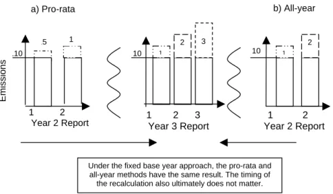
Using this example, Figure 2 then compares the all-year option with the pro-rata option, when using a fixed base year. It illustrates that there have to be two

recalculations when using the pro-rata option, after which the resulting time series of emissions and thus the comparison over time, is equivalent to the all year option, which only requires one recalculation.

Figure 2: An acquisition (example Z) under different fixed base year options

Using the pro-rata option, illustrated on the left of Figure 2, company A would when first reporting its year 2 emissions, report 11t, including only the emissions of B from June to December in year 2 (assumed to be 1t for simplicity). In order to compare like with like, it recalculates its base year emissions to 10.5 t, including in its base year emissions again only B s emissions from June to December (in year 1).

When reporting on year 3, A would then include emissions from January to December from B, and in order to keep comparing like with like, would have to make a second recalculation to its base year emissions, to include B s emissions from January to June in year 1. This results in exactly the same time series and comparison over time (in the middle) as under the all-year option, which is illustrated on the right (see also the shaded rows in table 1 to see that both approaches arrive at the same result). The all-year option is thus clearly more practicable than the pro-rata one.

Table 1: An acquisition (example Z) under different fixed base year options

Year 1 (Base year)

Year 2 Year 3 Year 4

Company A s emissions

(boundaries as in year 1)

10 10 10 10

Company B s emissions

(boundaries as in year 1)

1 2 3 3

Pro-rata approach

Company A s year 2 report 10.5 11

Company A s year 3 report 11 12 13

10 10

110

1 2

Year 2 Report 1 _{Year 3 Report} 2 3 _{Year 2 Report}1 2

.5

1

2

3

1

2

Under the fixed base year approach, the pro-rata and all-year methods have the same result. The timing of

the recalculation also ultimately does not matter.

a) Pro-rata b) All-year

E

m

is

s

io

n

s

(4)

Company A s year 2 report 11 12

Company A s year 3 report 11 12 13

Further differentiating methods for recalculation is possible when taking into account the timing of recalculation. It is possible to make the recalculation only in the report for the year after the structural change, i.e., as if the structural change had occurred at the end of the year (this could be termed the year-after option). The default option (if sufficient data is available) would be to make the recalculation already in the report for the year of the structural change, i.e. as if the structural change had occurred at the beginning of the year ( same-year option). Switching between these two options does not influence the ultimate comparison over time under the fixed base year, just as when comparing the pro-rata and the all-year options.

2 Target base year recalculation methodologies for structural

changes using a rolling base year

As described in chapter 11 of the revised Corporate Standard, the rolling base year approach requires making recalculations of base year emissions only for the previous year, since the base year with which current emissions are compared on a like with like basis is always the previous year. The rolling base year is another title for establishing a new base year every year.

As mentioned above, after recalculations under the fixed base year approach, emissions sources from an acquired company are included both with their emissions in the base year (when the acquiring company didn t control these sources yet) and in the current years. Similarly, emission sources from divested facilities/companies are excluded both with their emissions in the base year (when they were still controlled by the divesting company) and the current years.

This makes for an important difference to the rolling base year, since the rolling base year minimizes both the inclusion of emissions data from non-controlled sources (e.g., before these sources were acquired) and the exclusion of data from controlled sources (e.g., before these sources were divested). In this way, under the rolling approach, any comparison over time is purely focussed on emissions that were actually controlled or owned by the reporting company. 1

However, the extent to which this is achieved is not exactly the same for each of the possible rolling base year recalculation methods.

The point of this section is firstly to describe the application of each of these possible methods, and to show that each of them has slightly different implications for which data is included or excluded. Thus, unlike under the fixed base year, it does make a difference to emissions comparisons whether the pro-rata or all-year method is used. In addition, the timing of recalculations (using the year-after vs. the same-year option) can also change emissions comparisons over time.

The combination of these different options results in four possible methods for rolling base year recalculations. The next two sub-sections describe the application and

1

These and other differences are described in Figure 14 of the revised Corporate Standard (p.81)

(5)

implications of these four methods, for an acquisition and for a divestment respectively.

2.1 Recalculating a rolling base year for acquisitions

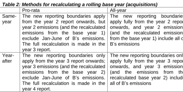
Table 2 builds on example Z and illustrates the four different methods of how a rolling base year is recalculated to account for an acquisition.

Table 2: Methods for recalculating a rolling base year (acquisitions)

Pro-rata All-year

Same-year

The new reporting boundaries apply from the year 2 report onwards, but year 2 emissions (and the recalculated emissions from the base year 1) exclude Jan-June of B s emissions. The full recalculation is made in the year 3 report.

The new reporting boundaries apply fully from the year 2 report onwards, and year 2 emissions (and the recalculated emissions from the base year 1) include all of B s emissions

Year-after

The new reporting boundaries only apply from the year 3 report onwards; year 3 emissions (and the recalculated emissions from the base year 2) exclude Jan-June of B s emissions. The full recalculation is made in the year 4 report.

The new reporting boundaries only apply fully from the year 3 report onwards, and year 3 emissions (and the emissions from the recalculated base year 2) include all of B s emissions

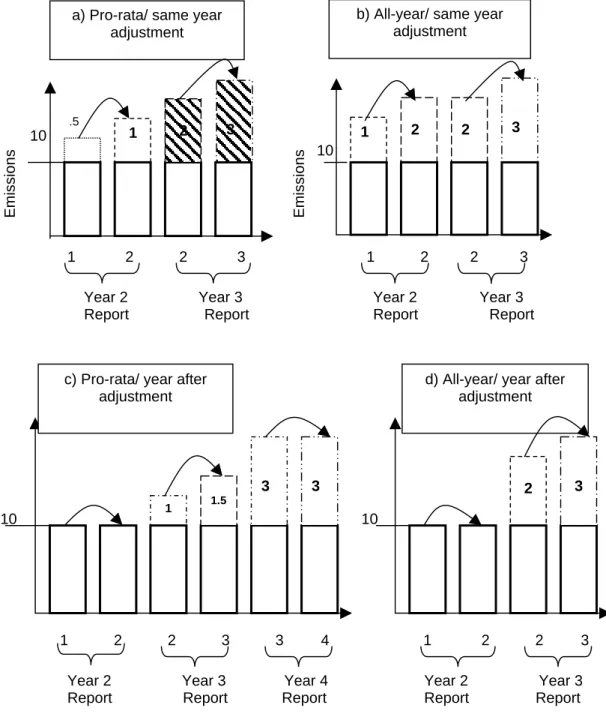
Figure 3 illustrates how each of the four recalculation methods outlined in Table 2 would be applied to example Z. Figure 3 also shows that each of the methods has different implications for the overall comparison of emissions over time (comparisons from year to year is what the arrows are indicating).

(6)

Figure 3: An acquisition (example Z) under different rolling base year methods

Why do the differences between methods matter under the rolling base year approach? An explanation is given in Table 3 below. It shows that each method has different implications in terms of whether the company includes emissions from sources that were not owned or controlled by it.

.5

d) All-year/ year after adjustment

10

10 10

1

2

a) Pro-rata/ same year adjustment

3

3 1

2

b) All-year/ same year adjustment

10

1

1.5

3

2

3

c) Pro-rata/ year after adjustment

1 2 2 3

E

m

is

s

io

n

s

E

m

is

s

io

n

s

1 2 2 3 3 4

1 2 2 3 Year 2 Year 3

Report Report

Year 2 Year 3 Report Report

Year 2 Year 3 Year 4 Report Report Report

(7)

Table 3 illustrates these implications by comparing what is included in A s inventory reports under each method and what was really owned or controlled by A (see Figure 4 for emissions from sources that A did control in respective years in example Z). As a basis for the comparison in table 3, figure 4 describes the emissions from sources that A did control in respective years in example Z. The actual emissions from sources owned or controlled by A are 10 in year 1 before the acquisition and 11 in year 2: only half of company B s annual emissions were controlled by A since it was acquired in June of year 2. From year 3 onwards, company A fully controlled its own operations and those of company B.

Figure 4: Emissions from sources controlled by A in respective years in example Z

Table 3: Implications of different rolling base year recalculation methods for acquisitions

Pro-rata All-year

Same-year

Half a year s data from B when not controlled are included;

(No data from B when controlled are excluded)

One and a half year s data from B when not controlled is included; (No data from B when controlled are excluded)

Year-after

No data from B when not controlled are included;

Half a year s data from B when not controlled are included;

These differences in what is included or excluded can in turn result in different comparisons over time under different methods. Thus, especially when setting and reporting in relation to a GHG target using a rolling base year, it is important to be transparent about which method is used, and to be consistent in the application of that method.

In addition to making a difference to the overall comparison over time, the choice of method also has implications for data requirements (the year-after methods usually require data from the acquired company at a later stage than the same-year

1 2 3 4 Year

13

11 10

(8)

2.2 Recalculating a rolling base year for divestments

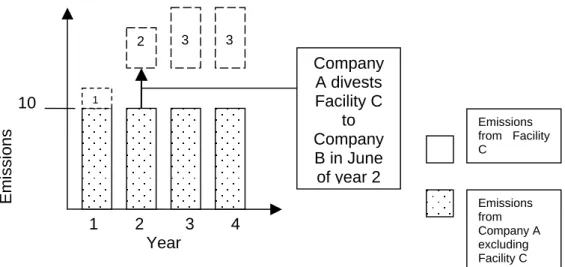
The analysis of section 2.1 is repeated here for the case of divestments. Example Y (Figure 5) is used in analogy to example Z: Company A divests a facility C to company B in the middle of year 2 on 30 June.

Figure 5: Example Y (divestment)

Table 4 builds on example Y and illustrates the four different methods of how a rolling base year is recalculated to account for a divestment.

Table 4: Methods for recalculating a rolling base year (divestments)

Pro-rata All-year

Same-year

The new reporting boundaries apply from the year 2 report onwards, but year 2 emissions (and the recalculated emissions from the base year 1) still include Jan-June of facility C s emissions. The full recalculation is made in the year 3 report

The new reporting boundaries apply fully from the year 2 report onwards, and year 2 emissions (and the recalculated emissions from the base year 1) exclude all of C s emissions

Year-after

The new reporting boundaries only apply from the year 3 report onwards; and year 3 emissions (and the recalculated emissions from the base year 2) still include Jan-June of C s emissions. The full recalculation is made in the year 4 report

The new reporting boundaries apply fully only from the year 3

report onwards, but year 3

emissions (and the emissions from the recalculated base year 2) exclude all of C s emissions

Figure 6 shows how each of the recalculation methods would be applied in the case of a divestment.

1 2 3 4 Year

E

m

is

s

io

n

s

1

2

3

10

Company A divests Facility C

to Company B in June of year 2

Emissions from Facility C

Emissions from Company A excluding Facility C

(9)

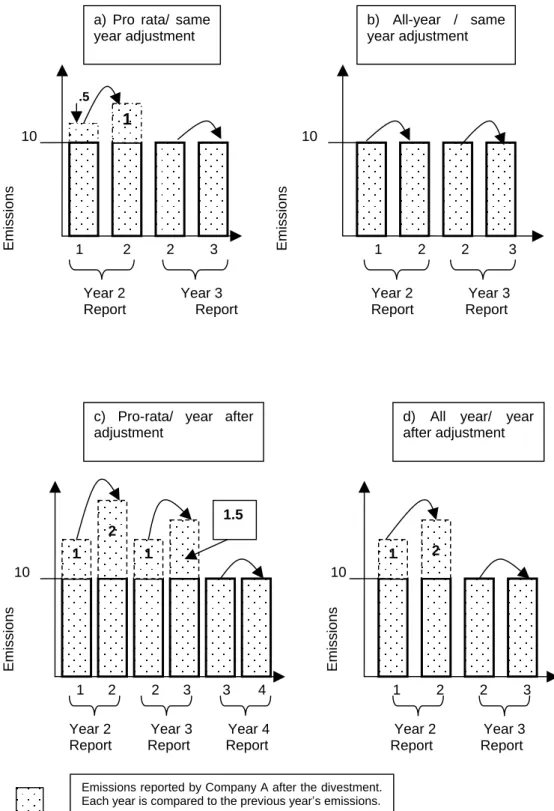
Figure 6: A divestment (example Y) under different rolling base year methods

Table 5 shows that each method has different implications in terms of whether the company excludes emissions from sources that were actually owned or controlled by it (and in fact in terms of whether the company includes emissions from sources that were not actually owned or controlled by it any more).

E

m

is

s

io

n

s

10

1 2 2 3

E

m

is

s

io

n

s

10

1 2 2 3 3 4

c) Pro-rata/ year after adjustment

1

2 1

1.5

d) All year/ year after adjustment

1

2

Year 2 Year 3 Year 4 Report Report Report

Emissions reported by Company A after the divestment. Each year is compared to the previous year s emissions.

E

m

is

s

io

n

s

1 2 2 3 1 2 2 3

10

.5

a) Pro rata/ same year adjustment

1

b) All-year / same year adjustment

E

m

is

s

io

n

s

10

(10)

It illustrates these implications by comparing what is included in A s inventory reports under each method and what was really owned or controlled by A.

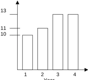
As a basis for the comparison in table 5, figure 7 describes the emissions from sources that A did control in respective years in example Y. The actual emissions from sources owned or controlled by A in example Y are 11 in year 1 before the divestment and also 11 in year 2: half of facility C s emissions were controlled by A in year 2 since the facility was divested in June of year 2. From year 3 onwards company A only controlled its own operations without facility C.

Figure 7: Emissions from sources controlled in respective years by A in example Y

Table 5: Implications of different rolling base year recalculation methods for divestments

Pro-rata All-year

Same-year

No data from C when not controlled are included;

Half a year s data from C when controlled are excluded;

No data from C when not controlled are included;

One and a half year s data from C when controlled are excluded;

Year-after

One year s data (two halves) from C when not controlled are included; No data from C when controlled are excluded

Half a year s data from C when not controlled are included;

No data from C when controlled are excluded;

These differences in what is excluded or included can in turn result in different comparisons over time under different methods (as shown in Figure 5). Thus, especially when setting and reporting in relation to a GHG target using a rolling base year, it is important to be transparent about which method is used.

1 2 3 4 Year

11 10