Flight simulation testing of a turbulence model based on a Synthetic
Eddy Method
Sergio Henriquez Huecas
[email protected] University of Liverpool Liverpool, United Kingdom
Prof. Mark White [email protected] University of Liverpool Liverpool, United Kingdom
Prof. George Barakos [email protected]
University of Glasgow Glasgow, United Kingdom
In the proposed paper, the results of piloted simulation testing of a new turbulence model for flight simulation will be presented. The aim of the tests will be to assess the feasibility of the model for flight simulation applications and identifying the effects on helicopter handling and pilot workload of the different turbulence parameters used in the model. In addition subjective pilot evaluation of the realism and usefulness of the induced turbulence will be collected.
As of now, there is no unified approach to the assessment of turbulence effects on rotorcraft operations or for severity mitigation through design, regulations or training. EASA certifications for small (CS – 27, [1]) and large (CS – 29, [2]) rotorcraft only establish the need to ensure controllability and structural resistance under expected gust conditions. ADS – 33 [3] sets yaw rate limits in response to step lateral gusts for all aircraft. For attitude hold control systems, Level 1 requires return to less than 10% of peak deviations in roll and pitch within 10s (20s for pitch under good visual conditions) after a pulse disturbance and same response bandwidth to disturbances as to pilot control inputs. For certification, disturbances shall be modelled as inputs to the actuator surfaces. There seems to be little supporting data for this criteria [4] and it is intended to be replaced by a disturbance response bandwidth criteria in the future [5]. Other requirements set limits on the environmental conditions aircraft are allowed to operate. The UK Civil Aviation Authority (CAA) establishes a maximum of 1.75m/s on standard deviation of vertical wind velocity over landing areas on offshore platforms to allow operations [6]. These limits were defined after a series of piloted and offline flight simulation studies using airwake data collected from wind tunnel tests [7] [8] and replace a previous requirement defining an absolute maximum vertical wind speed.
Such lack of unified criteria might partly be due to the fact that adequately modelling the interaction between a rotorcraft and its surrounding aerodynamic environment in real-time for piloted simulation has proved to be a challenging endeavour. The current state of the art is the use of stored time accurate airwake solutions which have been pre-computed using Computational Fluid Dynamics (CFD) tools and are accessed during simulated flight [9]. However, computational costs and storage requirements means that only a limited number of short duration airwake solutions will usually be available. To address some of these issues, stochastic turbulence models [10] can generate random, low intensity, high frequency turbulent flow in real time superimposed over lower fidelity airwake solutions.
Helicopter turbulence models are usually built around the implementation of Von Karman’s formula [11] or Dryden models [12] based on the assumption of a homogeneous, isotropic and frozen turbulence field that approaches towards the aircraft with its aerodynamic velocity [13]. However adaptation to the broad range of flight conditions and the inclusion of rotation effects when computing turbulence correlation between the different blade elements is necessary [14], [15]. A simpler approach was suggested by McFarland et al. in [16], by distributing a turbulent velocity field over the rotor plane across a number of stations and displacing it by one station at each time step. A three dimensional extension to this method was proposed by Ji et al. in [17]. This method however has limitations when flight or environmental conditions experience large changes within a small number of time steps. Finally Lusardi et al. [18] and Seher-Weiss et al. [19] describe the use of System Identification techniques from flight test measurements for modelling turbulence upsets as equivalent control inputs. These models however are valid only for the very specific combinations of aircraft, environmental conditions and flight task for which both flight test data and aircraft dynamics model are available and are therefore not broadly applicable.
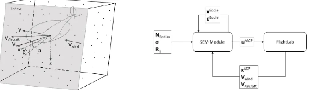
The turbulence model presented in this paper is proposed as a first step to solve some of these issues. It is based on a Synthetic Eddy Model (SEM) first proposed by Jarrin [20] to generate realistic turbulence oscillations at the inflow of CFD simulations. The detailed description and implementation of the model will be described in Ref [21]. A box–shaped control volume is defined around the aircraft and completely filled by a random uniform distribution of eddies, an inflow is defined facing towards the direction of the incoming aerodynamic velocity (see Figure 1). A prototype has been developed in Simulink and coupled with a FLIGHTLAB [22] helicopter model. The Simulink SEM module computes the turbulent flow velocities at a series of Airload Computation Points (ACPs) located around the airframe and rotor blades at each time step and transfers them to FLIGHTLAB which computes the resulting aircraft dynamics.
Figure 1: Left: Diagram of the control volume used for the synthetic eddy method. Right: Flow chart of data exchanged between the SEM module and FLIGHTLAB.
On each time step an eddy located on generates a turbulent velocity perturbation on an ACP located at . The total induced turbulence on each ACP is obtained by adding the contribution of each eddy: 1 √ ∑ )
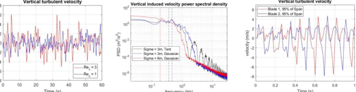
Where is a randomly assigned sign and A is the Cholesky decomposition of the Reynolds stress tensor ( 〈 〉 ), which controls the resulting turbulence intensity (see Figure 2 left). The shape function ) ) relates the shape and size of the eddies, , with the decay of their effect with distance and their adjustment defines the resulting turbulence spectra (see Figure 2 center). Values for these parameters can be obtained from measurements or CFD simulations [23], [24]. After each time step, the population of eddies is displaced with the wind velocity resulting in a random frozen turbulence field which displaces itself with ambient wind velocity. Eddies falling outside the control volume at the start of the time step are regenerated at a random location at the inflow.
The main advantage of SEM compared to previous turbulence models is that the location of the eddies near the aircraft is preserved for each time step. This ensures that turbulence induced for each ACP is coherent with the effects on the rest of the aircraft even if aircraft flight velocities experience large changes in a small number of time steps (see Figure 2 right). It also opens the possibility of coupling the displacement and parameters of the eddies with precomputed airwake solutions or with the aircraft’s own airwake, options that will be explored in the future.
In preparation for flight simulation tests, the SEM turbulence model has been coupled to a FLIGHTLAB Bell 412 aircraft model [25]. Offline simulations have been performed with the aircraft in hover with different configurations: all states frozen and the stability system deactivated as well as with a rate command attitude hold configured stability system and only the vertical axis frozen (to prevent the aircraft model from crashing). Turbulence effects in aircraft blade flapping, rotor thrust and moments are clearly appreciable within the 0.1 – 2Hz frequency range that affects aircraft and pilot handling [26] (see Figure 2 and Figure 3).
Figure 2: Time history of vertical component of turbulent velocity against Rii values. Center: PSD of vertical induced turbulent velocities against eddy shape and size. Vertical dashed lines indicate power spectral density averaged frequency. Right: Correlation between turbulence induced vertical flow velocities at the tip of opposite
blades.
Figure 3: Left: Power spectral density of main rotor blade flapping. Center: Power spectral density of main rotor thrust coefficient. Right: Power spectral density of pitch moments acting on aircraft.
Piloted flight simulation testing has focused on hover and low speed flight conditions to assess how different adjustments of the SEM induced turbulence affect aircraft handling, pilot response and workload. The pilot performed a precision hover task as defined [3] with the stability system configured for rate command and attitude control. Aircraft dynamics and pilot inputs have been recorded and subjective data gathered using the Bedford Workload [27] and Cooper Harper Handling Qualities rating scales [28] respectively. Additional pilot feedback and comments were also obtained during briefing, test and de-briefing.
Initial testing focussed on the following objectives:
Identifying turbulence intensity limits at which aircraft handling or motion based flight simulation is still feasible:
The pilot was tasked to perform the precision hover task starting from conditions of no turbulence, tests were repeated under increasingly higher levels of turbulence intensity until the task can no longer be completed, pilot workload becomes unreasonably high or the motion of the platform becomes excessive. All runs were performed using the smallest Eddy size feasible for real time simulation and therefore the highest possible frequency.
Assessing the effect of turbulence frequency on handling:
From the previous tests a suitable level of turbulence intensity was chosen and a series of runs performed maintaining turbulence intensity but increasing Eddy size. The turbulence spectra and resulting disturbances will shift towards lower frequencies. A second suitable Eddie Size was tested for different turbulence intensities.
Assessing the effect of different distributions of Eddy sizes:
For the same turbulence intensity selected on the first phase, the turbulence was dispersed across different Eddy sizes ranging from 3m to larger sizes. The criteria chosen is to scale the value of Reynolds Stress Tensors in proportion to Eddie Length scale.
Assessing the effect of different Eddie shapes:
For the chosen turbulence intensity and Eddy size, a series of runs was performed switching the function describing Eddy strength decay with distance between a tent shaped function and Gaussian shaped functions with different decay values.
Analysis of the results will inform the conditions and mission tasks elements to be performed for following tests. Priority will be the assessment of turbulence at a range of different aircraft flight speeds by performing a custom steady flight task, with desired and adequate limits for heading, lateral deviations and altitude being the same as for the acceleration – deceleration task as defined by ADS – 33 and allowable velocity deviations have been defined as 5kts (desired) or 10kts (adequate).
References
[1] CS - 27 Certification Specifications and Acceptable Means of Compliance for Small Rotorcraft. European Aviation Safety Agency, 2016.
[2] CS - 29 Certification Specifications and Acceptable Means of Compliance for Large Rotorcraft. European Aviation Safety Agency, 2016.
[3] “Aeronautical Design Standards - Performance Specification Handling Qualities Requirements for Military Rotorcraft,” United States Army Aviation and Missile Command, vol. E-PRF, 2000. [4] R. H. Hoh, D. G. Mitchell, B. L. Aponso, D. L. Key, and C. Blanken L., “Special Report
RDMR-AD-16-01: Background Information and User’s Guide for Handling Qualities Requirements for Military Rotorcraft,” Aviation Development Directorate, Ames Research Center, 1989.
[5] T. Berger, C. M. Ivler, M. G. Berrios, M. B. Tischler, and D. G. Miller, “Disturbance Rejection Handling Qualities Criteria for Rotorcraft,” American Helicopter Society 72nd Annual Forum, West Palm Beach, FL, 2016.
[6] UK Civil Aviation Authority, “CAP 437 Standards for Offshore Helicopter Landing Areas,” p. 164, 2013.
[7] Safety Regulation Group CAA, “CAA PAPER 2004/03 Helicopter Turbulence Criteria for Operations to Offshore Platforms,” 2004.
[8] “CAA Paper 2009 / 03: Offshore Helideck Environmental Research Part,” 2009.
[9] I. Owen, M. D. White, G. D. Padfield, and S. J. Hodge, “A virtual engineering approach to the ship-helicopter dynamic interface – a decade of modelling and simulation research at the University of Liverpool,” The Aeronautical Journal, vol. 121, no. 1246, pp. 1833–1857, Dec. 2017.
[10] G. H. Gaonkar, “Review of Turbulence Modeling and Related Applications to Some Problems of Helicopter Flight Dynamics,” Journal of the American Helicopter Society, vol. 53, no. 1, p. 87, 2008.
[11] T. von Karman, “Progress in the Statistical Theory of Turbulence,” Proceedings of the National Academy of Sciences, vol. 34, no. 11, pp. 530–539, Nov. 1948.
[12] H. L. Dryden, “A review of the statistical theory of turbulence,” Quarterly of Applied Mathematics, vol. 1, no. 1, pp. 7–42, Apr. 1943.
[13] B. Etkin, “Turbulent Wind and Its Effect on Flight,” Journal of Aircraft, vol. 18, no. 5, pp. 327– 345, 2008.
[14] Mark F. Costello, “A Theory for the Analysis of Rotorcraft Operating In Atmospheric Turbulence,” American Helicopter Society 46th Annual Forum, 1990.
[15] Y. Y. Dang, S. Subramanian, and G. H. Gaonkar, “Modeling Turbulence Seen by Multibladed Rotors for Predicting Rotorcraft Response with Three-Dimensional Wake,” Journal of the American Helicopter Society, vol. 42, no. 4, pp. 337–349, 2009.
[16] R. E. Mcfarland and K. Duisenberg, “NASA Technical Memorandum 108862: Simulation of rotor blade element turbulence,” Moffett Field, CA, 1995.
[17] H. Ji, R. Chen, and P. Li, “Distributed atmospheric turbulence model for helicopter flight simulation and handling-quality analysis,” Journal of Aircraft, vol. 54, no. 1, pp. 190–198, 2017. [18] J. A. Lusardi, M. B. Tischler, C. L. Blanken, and S. J. Labows, “Empirically Derived Helicopter
Response Model and Control System Requirements for Flight in Turbulence,” Journal of the American Helicopter Society, vol. 49, no. 3, pp. 340–349, 2009.
[19] S. Seher-Weiss and W. Von Gruenhagen, “Development of EC 135 turbulence models via system identification,” Aerospace Science and Technology, vol. 23, no. 1, pp. 43–52, 2012. [20] N. Jarrin, S. Benhamadouche, D. Laurence, and R. Prosser, “A synthetic-eddy-method for
generating inflow conditions for large-eddy simulations,” International Journal of Heat and Fluid Flow, vol. 27, no. 4, pp. 585–593, 2006.
[21] S. Henriquez Huecas, M. White, and G. Barakos, “A turbulence model for flight simulation and handling qualities analysis based on a synthetic eddy method,” To be presented at 76th Vertical Flight Society Forum, Virginia Beach, VA, 2020.
[22] R. W. Du Val and C. He, “Validation of the FLIGHTLAB virtual engineering toolset,” The Aeronautical Journal, vol. 122, no. 1250, pp. 519–555, Apr. 2018.
[23] N. Jarrin, R. Prosser, J. C. Uribe, S. Benhamadouche, and D. Laurence, “Reconstruction of turbulent fluctuations for hybrid RANS/LES simulations using a Synthetic-Eddy Method,” International Journal of Heat and Fluid Flow, vol. 30, no. 3, pp. 435–442, 2009.
[24] Y. Luo, H. Liu, Q. Huang, H. Xue, and K. Lin, “A multi-scale synthetic eddy method for generating inflow data for LES,” Computers and Fluids, vol. 156, pp. 103–112, 2017.
[25] P. Perfect, M. D. White, G. D. Padfield, and A. W. Gubbels, “Rotorcraft simulation fidelity: new methods for quantification and assessment,” The Aeronautical Journal, vol. 117, no. 1189, pp. 235–282, 2013.
[26] G. D. Padfield, Helicopter Flight Dynamics, 2nd ed. Blackwell Publishing, 1996.
[27] A. H. Roscoe and A. H. Ellis, “Technical Report TR 90019: A subjective rating scale for assessing pilot workload in flight: A decade of practical use,” Royal Aerospace Establishment, 1990.
[28] G. E. Cooper and R. P. Harper, “NASA Tecnical Note: TN-D-5153: The use of pilot rating in the evaluation of aircraft handling qualities,” Moffett Field, CA, 1969.