Large-Scale Quadratically Constrained Quadratic
Program via Low-Discrepancy Sequences
Kinjal Basu, Ankan Saha, Shaunak Chatterjee LinkedIn Corporation
Mountain View, CA 94043
{kbasu, asaha, shchatte}@linkedin.com
Abstract
We consider the problem of solving a large-scale Quadratically Constrained Quadratic Program. Such problems occur naturally in many scientific and web applications. Although there are efficient methods which tackle this problem, they are mostly not scalable. In this paper, we develop a method that transforms the quadratic constraint into a linear form by sampling a set of low-discrepancy points [16]. The transformed problem can then be solved by applying any state-of-the-art large-scale quadratic programming solvers. We show the convergence of our ap-proximate solution to the true solution as well as some finite sample error bounds. Experimental results are also shown to prove scalability as well as improved quality of approximation in practice.
1
Introduction
In this paper we consider the class of problems called quadratically constrained quadratic program-ming (QCQP) which take the following form:
Minimize x 1 2x TP 0x+qT0x+r0 subject to 1 2x TP ix+qTi x+ri≤0, i= 1, . . . , m (1) Ax=b,
where P0, . . . ,Pm aren×nmatrices. If each of these matrices are positive definite, then the
optimization problem is convex. In general, however, solving QCQP is NP-hard, which can be verified by easily reducing a0−1integer programming problem (known to be NP-hard) to a QCQP [4]. In spite of that challenge, they form an important class of optimization problems, since they arise naturally in many engineering, scientific and web applications. Two famous examples of QCQP include the max-cut and boolean optimization [11]. Other examples include alignment of kernels in semi-supervised learning [29], learning the kernel matrix in discriminant analysis [28] as well as more general learning of kernel matrices [21], steering direction estimation for radar detection [15], several applications in signal processing [20], the triangulation in computer vision [3] among others. Internet applications handling large scale of data, often model trade-offs between key utilities using constrained optimization formulations [1,2]. When there is independence among the expected utilities (e.g., click, time spent, revenue obtained) of items, the objective or the constraints corresponding to those utilities are linear. However, in most real life scenarios, there is dependence among expected utilities of items presented together on a web page or mobile app. Examples of such dependence are abundant in newsfeeds, search result pages and most lists of recommendations on the internet. If this dependence is expressed through a linear model, it makes the corresponding objective and/or constraint quadratic. This makes the constrained optimization problem a very large scale QCQP, if
the dependence matrix (often enumerated by a very large number of members or updates) is positive definite with co-dependent utilities [6].
Although there are a plethora of such applications, solving this problem on a large scale is still extremely challenging. There are two main relaxation techniques that are used to solve a QCQP, namely, semi-definite programming (SDP) and reformulation-linearization technique (RLT) [11]. However, both of them introduce a new variableX=xxT so that the problem becomes linear inX. Then they relax the conditionX=xxT by different means. Doing so unfortunately increases the
number of variables fromntoO(n2). This makes these methods prohibitively expensive for most
large scale applications. There is literature comparing these methods which also provides certain combinations and generalizations[4,5,22]. However, they all suffer from the same curse of dealing withO(n2)variables. Even when the problem is convex, there are techniques such as second order
cone programming [23], which can be efficient, but scalability still remains an important issue with prior QCQP solvers.
The focus of this paper is to introduce a novel approximate solution to the convex QCQP problem which can tackle such large-scale situations. We devise an algorithm which approximates the quadratic constraints by a set of linear constraints, thus converting the problem into a quadratic program (QP) [11]. In doing so, we remain with a problem havingnvariables instead ofO(n2). We
then apply efficient QP solvers such as Operator Splitting or ADMM [10,26] which are well adapted for distributed computing, to get the final solution for problems of much larger scale. We theoretically prove the convergence of our technique to the true solution in the limit. We also provide experiments comparing our algorithm to existing state-of-the-art QCQP solvers to show comparative solutions for smaller data size as well as significant scalability in practice, particularly in the large data regime where existing methods fail to converge. To the best of our knowledge, this technique is new and has not been previously explored in the optimization literature.
Notation:Throughout the paper, bold small case letters refer to vectors while bold large-case letters refer to matrices.
The rest of the paper is structured as follows. In Section2, we describe the approximate problem, important concepts to understand the sampling scheme as well as the approximation algorithm to convert the problem into a QP. Section3contains the proof of convergence, followed by the experimental results in Section4. Finally, we conclude with some discussion in Section5.
2
QCQP to QP Approximation
For sake of simplicity throughout the paper, we deal with a QCQP having a single quadratic constraint. The procedure detailed in this paper can be easily generalized to multiple constraints. Thus, for the rest of the paper, without loss of generality we consider the problem of the form,
Minimize x (x−a) TA(x −a) subject to (x−b)TB(x−b)≤˜b, (2) Cx=c.
This is a special case of the general formulation in (1). For this paper, we restrict our case toA,
B∈Rn×nbeing positive definite matrices so that the objective function is strongly convex.
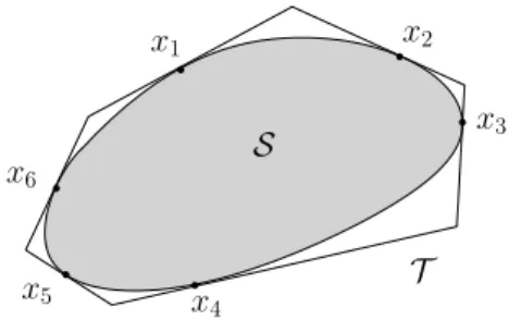
In this section, we describe the linearization technique to convert the quadratic constraint into a set of Nlinear constraints. The main idea behind this approximation, is the fact that given any convex set in the Euclidean plane, there exists a convex polytope that covers the set. Let us begin by introducing a few notations. LetPdenote the optimization problem (2). Define,
S :={x∈Rn : (x−b)TB(x−b)≤˜b}. (3)
Let∂Sdenote the boundary of the ellipsoidS. To generate theN linear constraints for this one quadratic constraint, we generate a set ofNpoints,XN ={x1, . . . ,xN}such that eachxj∈∂Sfor
j= 1, . . . , N . The sampling technique to select the point set is given in Section2.1. Corresponding to theseNpoints we get the following set ofNlinear constraints,
(x−b)TB(xj−b)≤˜b forj= 1, . . . , N. (4) Looking at it geometrically, it is not hard to see that each of these linear constraints are just tangent planes toSatxj forj = 1, . . . , N. Figure1shows a set of six linear constraints for a ellipsoidal
feasible set in two dimensions. Thus, using theseNlinear constraints we can write the approximate optimization problem,P(XN), as follows.
Minimize x (x−a) TA(x −a) subject to (x−b)TB(xj−b)≤˜b forj= 1, . . . , N (5) Cx=c.
Now instead of solvingP, we solveP(XN)for a large enough value ofN. Note that as we sample
more points (N→ ∞), our approximation keeps getting better.
x1 x2 x3 x4 x5 x6 S T
Figure 1: Converting a quadratic constraint into linear constraints. The tangent planes through the 6 pointsx1, . . . ,x6create the approximation toS.
2.1 Sampling Scheme
The accuracy of the solution ofP(XN)solely depends on the choice ofXN. The tangent planes to Sat thoseN points create a cover ofS. We use the notion of a bounded cover, which we define as follows.
Definition 1. Let T be the convex polytope generated by the tangent planes toS at the points
x1, . . . ,xN ∈∂S.T is said to be a bounded cover ofSif,
d(T,S) := sup
t∈T
d(t,S)<∞,
whered(t,S) := infx∈Skt−xkandk · kdenotes the Euclidean distance. The first result shows that there exists a bounded cover with onlyn+ 1points.
Lemma 1. LetSbe andimensional ellipsoid as defined in(3). Then there exists a bounded cover withn+ 1points.
Proof. Note that sinceSis a compact convex body inRn, there exists a location translated version of
ann-dimensional simplexT ={x∈Rn
+:
Pn
i=1xi =K}such thatSis contained in the interior of
T. We can always shrinkT such that each edge touchesStangentially. Since there aren+ 1faces, we will getn+ 1points whose tangent surface creates a bounded cover.
Although Lemma1gives a simple constructive proof of a bounded cover, it is not what we are truly interested in. What we want is to construct a bounded coverT which is as close as possible toS, thus leading to a better approximation. However note that, choosing the points via a naive sampling can lead to arbitrarily bad enlargements of the feasible set and in the worst case might even create a cover which is not bounded. Hence we need an optimal set of points which creates an optimal bounded cover. Formally,
Definition2. T∗=T(x∗1, . . . ,x∗N)is said to be an optimal bounded cover, if
sup
t∈T∗
d(t,S)≤sup
t∈T d(t,S)
for any bounded coverT generated by any otherN-point sets. Moreover,{x∗1, . . . ,x∗N}are defined
to be the optimalN-point set.
Note that we can think of the optimal N-point set as that set of N points which minimize the maximum distance betweenT andS, i.e.
T∗= argmin
T
It is not hard to see that the optimalN-point set on the unit circle in two dimensions are theN-th roots of unity, unique up to rotation. This point set also has a very good property. It has been shown that theN-th roots of unity minimize the discrete Riesz energy for the unit circle [14,17]. The concept of Reisz energy also exists in higher dimensions. Thus, generalizing this result, we choose our optimalN-point set on∂Swhich tries to minimize the Reisz energy. We briefly describe it below. 2.1.1 Riesz Energy
Riesz energy of a point setAN ={x1, . . . ,xN}is defined asEs(AN) :=P N
i6=j=1kxi−xjk−
sfor
a positive real parameters. There is a vast literature on Riesz energy and its association with “good” configuration of points. It is well known that the measures associated to the optimal point set that minimizes the Riesz energy on∂Sconverge to the normalized surface measure of∂S[17]. Thus using this fact, we can associate the optimalN-point set to the set ofN points that minimize the Riesz energy on∂S. For more details see [18,19] and the references therein. To describe these good configurations of points, we introduce the concept of equidistribution. We begin with a “good” or equidistributed point set in the unit hypercube (described in Section2.1.2) and map it to∂Ssuch that the equidistribution property still holds (described in Section2.1.3).
2.1.2 Equidistribution
Informally, a set of points in the unit hypercube is said to be equidistributed, if the expected number of points inside any axis-parallel subregion, matches the true number of points. One such point set in[0,1]nis called the(t, m, n)-net in baseη, which is defined as a set ofN =ηmpoints in[0,1]n
such that any axis parallelη-adic box with volumeηt−mwould contain exactlyηtpoints. Formally, it is a point set that can attain the optimal integration error ofO((log(N))n−1/N)[16] and is usually
referred to as alow-discrepancypoint set. There is vast literature on easy construction of these point sets. For more details on nets we refer to [16,24].
2.1.3 Area preserving map to∂S
Now once we have a point set on[0,1]nwe try to map it to∂Susing a measure preserving transfor-mation so that the equidistribution property remains intact. We describe the mapping in two steps. First we map the point set from[0,1]nto the hyper-sphere
Sn={x∈Rn+1:xTx= 1}. Then we
map it to∂S. The mapping from[0,1]ntoSnis based on [12].
The cylindrical coordinates of then-sphere, can be written as
x=xn= (p1−t2
nxn−1, tn), . . . , x2= (
q 1−t2
2x1, t2), x1= (cosφ,sinφ)
where0≤φ≤2π,−1≤td≤1,xd∈Sdandd= (1, . . . , n). Thus, an arbitrary pointx∈Sncan
be represented through angleφand heightst2, . . . , tnas,
x=x(φ, t2, . . . , tn), 0≤φ≤2π,−1≤t2, . . . , tn≤1.
We map a pointy= (y1, . . . , yn)∈[0,1)ntox∈Snusing
ϕ1(y1) = 2πy1, ϕd(yd) = 1−2yd (d= 2, . . . , n)
and cylindrical coordinates x = Φn(y) = x(ϕ1(y1), ϕ2(y2), . . . , ϕn(yn)). The fact that Φn : [0,1)n
→Snis an area preserving map has been proved in [12].
Remark. Instead of using (t, m, n)-nets and mapping to Sn, we could have also used spherical
t-designs, the existence of which was proved in [9]. However, construction of such sets is still a tough problem in high dimensions. We refer to [13] for more details.
Finally, we consider the mapψto translate the point set fromSn−1to∂S. Specifically we define,
ψ(x) =p˜bB−1/2x+b. (6)
From the definition ofSin (3), it is easy to see thatψ(x)∈∂S. The next result shows that this is also an area-preserving map, in the sense of normalized surface measures.
Lemma 2. Letψbe a mapping fromSn−1→∂Sas defined in(6). Then for any setA⊆∂S,
σn(A) =λn(ψ−1(A))
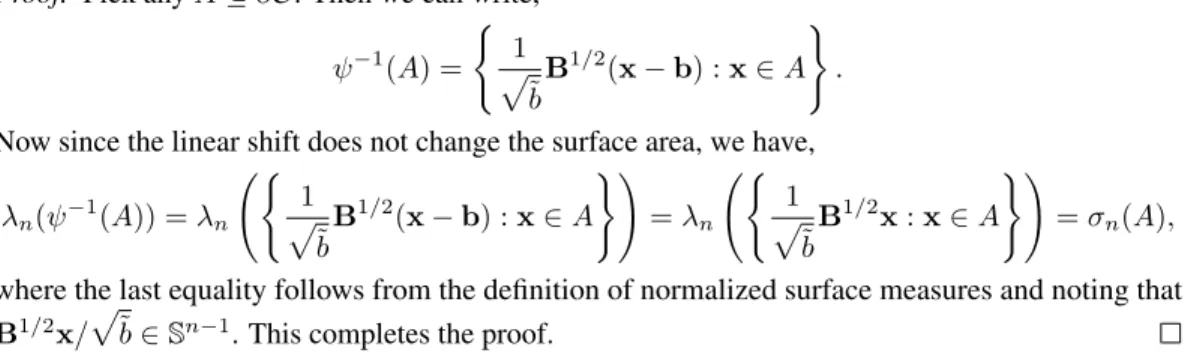
Proof. Pick anyA⊆∂S. Then we can write, ψ−1(A) = ( 1 p ˜ b B1/2(x−b) :x∈A ) . Now since the linear shift does not change the surface area, we have,
λn(ψ−1(A)) =λn ( 1 p ˜ b B1/2(x−b) :x∈A )! =λn ( 1 p ˜bB 1/2x:x ∈A )! =σn(A), where the last equality follows from the definition of normalized surface measures and noting that
B1/2x/p˜b∈
Sn−1. This completes the proof.
Using Lemma2we see that the mapψ◦Φn−1 : [0,1)n−1 → ∂S,is a measure preserving map.
Using this map and the(t, m, n−1)net in baseη, we derive the optimalηm-point set on∂
S. Figure
2shows how we transform a(0,7,2)-net in base 2 to a sphere and then to an ellipsoid. For more general geometric constructions we refer to [7,8].
Figure 2: The left panel shows a(0,7,2)-net in base2which is mapped to a sphere in 3 dimensions (middle panel) and then mapped to the ellipsoid as seen in the right panel.
2.2 Algorithm and Efficient Solution
From the description in the previous section we are now at a stage to describe the approximation algorithm. We approximate the problemP byP(XN)using a set of pointsx1, . . . ,xN as described
in Algorithm1. Once we formulate the problemP asP(XN), we solve the large scale QP via
Algorithm 1Point Simulation on∂S
1: Input :B,b,˜bto specifySandN =ηmpoints
2: Output :x1, . . . ,xN ∈∂S
3: Generatey1, . . . ,yN as a(t, m, n−1)-net in baseη.
4: fori∈1, . . . , Ndo
5: xi=ψ◦Φn−1(yi)
6: end for
7: returnx1, . . . ,xN
state-of-the-art solvers such as Operator Splitting or Block Splitting approaches [10,25,26].
3
Convergence of
P
(
X
N)
to
P
In this section, we shall show that if we follow Algorithm1to generate the approximate problem
P(XN), then we converge to the original problemPasN → ∞. We shall also prove some finite
Letx∗,x∗(N)denote the solution toPandP(XN)respectively andf(·)denote the strongly convex
objective function in (2), i.e., for ease of notation
f(x) = (x−a)TA(x−a). We begin with our main result.
Theorem 1. LetPbe the QCQP defined in(2)andP(XN)be the approximate QP problem defined in
(5)via Algorithm1. Then,P(XN)→ PasN → ∞in the sense thatlimN→∞kx∗(N)−x∗k= 0. Proof. Fix anyN. LetTN denote the optimal bounded cover constructed withN points on∂S. Note
that to prove the result, it is enough to show thatTN → SasN → ∞. This guarantees that linear
constraints ofP(XN)converge to the quadratic constraint ofP, and hence the two problems match.
Now sinceS ⊆ TN for allN, it is easy to see thatS ⊆limN→∞TN.
To prove the converse, lett0 ∈ limN→∞TN butt0 6∈ S. Thus,d(t0,S)> 0. Lett1denote the
projection oft0ontoS. Thus,t0 =6 t1 ∈ ∂S. Chooseto be arbitrarily small and consider any
regionAaroundt1on∂Ssuch thatd(x, t1)≤for allx∈A. Hereddenotes the surface distance
function. Now, by the equidistribution property of Algorithm1asN → ∞, there exists a point t∗∈A, the tangent plane through which cuts the plane joiningt0andt1. Thus,t06∈limN→∞TN.
Hence, we get a contradiction and the result is proved.
As a simple Corollary to Theorem1it is easy to see that aslimN→∞|f(x∗(N))−f(x∗)|= 0.We now move to some finite sample results.
Theorem 2. Letg :N→Rsuch thatlimn→∞g(n) = 0.Further assume thatkx∗(N)−x∗k ≤ C1g(N)for some constantC1 > 0. Then,|f(x∗(N))−f(x∗)| ≤ C2g(N)whereC2 > 0is a
constant.
Proof. We begin by bounding thekx∗k. Note that sincex∗satisfies the constraint of the optimization problem, we have,˜b≥(x∗−b)TB(x∗−b)≥σmin(B)kx∗−bk2, whereσmin(B)denotes the
smallest singular value ofB. Thus,
kx∗k ≤ kbk+ s
˜b
σmin(B)
. (7)
Now, sincef(x) = (x−a)TA(x
−a)and∇f(x) = 2A(x−a), we can write f(x) =f(x∗) + Z 1 0 h∇ f(x∗+t(x−x∗)),x−x∗idt =f(x∗) +h∇f(x∗),x−x∗i+ Z 1 0 h∇ f(x∗+t(x−x∗))− ∇f(x∗),x−x∗idt =I1+I2+I3(say).
Now, we can bound the last term as follows. Observe that using Cauchy-Schwarz inequality,
|I3| ≤ Z 1 0 |h∇ f(x∗+t(x−x∗))− ∇f(x∗),x−x∗i|dt ≤ Z 1 0 k∇ f(x∗+t(x−x∗))− ∇f(x∗)kkx−x∗kdt ≤2σmax(A) Z 1 0 k t(x−x∗)kkx−x∗kdt=σmax(A)kx−x∗k2,
whereσmax(A)denotes the largest singular value ofA. Thus, we have
f(x) =f(x∗) +h∇f(x∗),x−x∗i+ ˜Ckx−x∗k2 (8) where|C˜| ≤σmax(A). Furthermore,
|h∇f(x∗),x∗(N)−x∗i|=|h2A(x∗−a),x∗(N)−x∗i| ≤2σmax(A)(kx∗k+kak)kx∗(N)−x∗k ≤2C1σmax(A) s ˜b σmin(B) +kbk+kak g(N), (9)
where the last line inequality follows from (7). Combining (8) and (9) the result follows.
Note that the functionggives us an idea about how fastx∗(N)convergesx∗. To help, identify the functiongwe state the following results.
Lemma 3. Iff(x∗) = f(x∗(N)), thenx∗ =x∗(N). Furthermore, iff(x∗)≥f(x∗(N)), then
x∗∈∂Uandx∗(N)6∈ U, whereU =S ∩ {x:Cx=c}is the feasible set for(2).
Proof. LetV =TN∩ {x:Cx=c}. It is easy to see thatU ⊆ V. Assumef(x∗) =f(x∗(N)), but x∗6=x∗(N). Note thatx∗,x∗(N)∈ V. SinceVis convex, consider a line joiningx∗andx∗(N). For any pointλt=tx∗+ (1−t)x∗(N),
f(λt)≤tf(x∗) + (1−t)f(x∗(N)) =f(x∗(N)).
Thus,f is constant on the line joiningx∗andx∗(N). But, it is known thatf is strongly convex sinceAis positive definite [27]. Thus, there exists only one unique minimum. Hence, we have a contradiction, which provesx∗ =x∗(N).Now let us assume thatf(x∗)≥f(x∗(N)). Clearly,
x∗(N)6∈ U. Supposex∗ ∈U◦, the interior ofU. Let˜x∈∂U denote the point on the line joining
x∗andx∗(N). Clearly,˜x=tx∗+ (1−t)x∗(N)for somet >0. Thus,f(˜x) < tf(x∗) + (1− t)f(x∗(N))≤f(x∗). Butx∗is the minimizer overU. Thus, we have a contradiction, which gives
x∗∈∂U. This completes the proof.
Lemma 4. Following the notation of Lemma3, ifx∗(N)6∈ U, thenx∗lies on∂Uand no point on the line joiningx∗andx∗(N)lies inS.
Proof. Since the gradient offis linear, the result follows from a similar argument to Lemma3.
Based on the above two results we can identify the functiongby considering the maximum distance of the points lying on the conic cap to the hyperplanes forming it. That isg(N)is the maximum distance between a pointx∈∂Sand a point int∈ T such the line joiningxandtdo not intersect
Sand hence, lie completely within the conic section. This is highly dependent on the shape ofSand on the coverTN. For example, ifSis the unit circle in two dimensions, then the optimalN-point set
are theN-th roots of unity. In which case, there areNequivalent conic sectionsC1, . . . ,CN which
are created by the intersections of∂SwithTN. Figure3elaborates these regions.
C1 C2
C3
C4
C5
C6 π/6
Figure 3: The shaded region shows the 6 equivalent conic regions,C1, . . . ,C6.
To formally defineg(N)in this situation, let us defineA(t,x)to be the set of all points in the line joiningt∈ T andx∈∂S. Now, it is easy to see that,
g(N) := max
i=1,...,Nt,x:Asup(t,x)∈Cikt−xk= tan
π N =O 1 N , (10)
where the bound follows from using the Taylor series expansion oftan(x). Combining this observa-tion with Theorem2shows that in order to get an objective value withinof the true optimal, we would needNto be a constant multiplier of−1. More such results can be achieved by such explicit
4
Experimental Results
We compare our proposed technique to the current state-of-the-art solvers of QCQP. Specifically, we compare it to the SDP and RLT relaxation procedures as described in [4]. For small enough problems, we also compare our method to the exact solution by interior point methods. Furthermore, we provide empirical evidence to show that our sampling technique is better than other simpler sampling procedures such as uniform sampling on the unit square or on the unit sphere and then mapping it subsequently to our domain as in Algorithm1. We begin by considering a very simple QCQP for the form
Minimize x x TAx subject to (x−x0)TB(x−x0)≤˜b, l≤x≤u. (11)
We randomly sampleA,B,x0and˜bkeeping the problem convex. The lower bound,land upper
boundsuare chosen in a way such that they intersect the ellipsoid. We vary the dimensionnof the problem and tabulate the final objective value as well as the time taken for the different procedures to converge in Table1. The stopping criteria throughout our simulation is same as that of Operator Splitting algorithm as presented in [26].
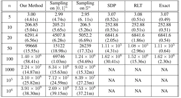
Table 1: The Optimal Objective Value and Convergence Time
n Our Method Sampling Sampling SDP RLT Exact
on[0,1]n on Sn 5 3.00 2.99 2.95 3.07 3.08 3.07 (4.61s) (4.74s) (6. 11s) (0.52s) (0.51s) (0.49) 10 206.85 205.21 206.5 252.88 252.88 252.88 (5.04s) (5.65s) (5.26s) (0.53s) (0.51s) (0.51) 20 6291.4 4507.8 5052.2 6841.6 6841.6 6841.6 (6.56s) (6.28s) (6.69s) (2.05s) (1.86s) (0.54) 50 99668 15122 26239 1.11×10 5 1.08 ×10⁵ 1.11×10⁵ (15.55s) (18.98s) (17.32s) (4.31s) (2.96s) (0.64) 100 1.40×10 6 69746 1.24 ×10⁶ 1.62 ×10⁶ 1.52 ×10⁶ 1.62 ×10⁶ (58.41s) (1.03m) (54.69s) (30.41s) (15.36s) (2.30s) 1000 2.24×10 7 8.34 ×10⁶ 9.02 ×10⁶ NA NA NA (14.87m) (15.63m) (15.32m) 105 3.10×10⁸ 7.12×10⁷ 8.39×10⁷ NA NA NA (25.82m) (24.59m) (27.23m) 106 3.91×10⁹ 2.69×10⁸ 7.53×10⁸ NA NA NA (38.30m) (39.15m) (37.21m)
Throughout our simulations, we have chosenη = 2and the number of optimal points asN = max(1024,2m), wheremis the smallest integer such that2m
≥10n. Note that even though the SDP and the interior point methods converge very efficiently for small values ofn, they cannot scale to values ofn ≥1000, which is where the strength of our method becomes evident. From Table1we observe that the relaxation procedures SDP and RLT fail to converge within an hour of computation time forn≥1000, whereas all the approximation procedures can easily scale up to n= 106variables. Moreover, since theA,Bwere randomly sampled, we have seen that the true optimal solution occurred at the boundary. Therefore, relaxing the constraint to linear forced the solution to occur outside of the feasible set, as seen from the results in Table1as well as from Lemma
3. However, that is not a concern, since increasingN will definitely bring us closer to the feasible set. The exact choice ofNdiffers from problem to problem but can be computed as we did with the small example in (10). Finally, the last column in Table1is obtained by solving the problem using cvxin MATLAB using via SeDuMi and SDPT3, which gives the truex∗.
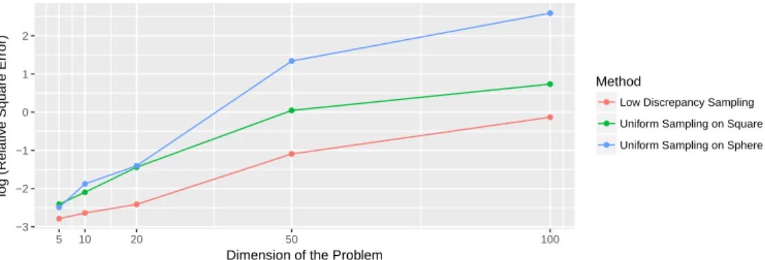
Furthermore, our procedure gives the best approximation result when compared to the remaining two sampling schemes. Lemma3shows that if the both the objective values are the same then we indeed get the exact solution. To see how much the approximation deviates from the truth, we also plot the log of the relative squared error, i.e.log(kx∗(N)−x∗k2/kx∗k2)for each of the sampling
procedures in Figure4. Throughout this simulation, we keepN fixed at 1024. This is why we see that the error level increases with the increase in dimension. We omit SDP and RLT results in Figure
−3 −2 −1 0 1 2 5 10 20 50 100
Dimension of the Problem
log (Relativ
e Square Error)
Method
Low Discrepancy Sampling Uniform Sampling on Square Uniform Sampling on Sphere
Figure 4: The log of the relative squared errorlog(kx∗(N)−x∗k2/kx∗k2)withN fixed at 1024 and varying dimensionn.
4since both of them produce a solution very close to the exact minimum for smalln. If we grow this Nwith the dimension, then we see that the increasing trend vanishes and we get much more accurate results as seen in Figure5. We plot both the log of relative squared error as well as the log of the feasibility error, where the feasibility error is defined as
Feasibility Error =(x∗(N)−x0)TB(x∗(N)−x0)−˜b
+
where(x)+denotes the positive part ofx.
−16 −14 −12 −10 −8 −6 −4 −2 2 3 4 5 6 7 log(Number of Constraints) log(Relativ e Squared Error) Dimension 5 10 20 −6 −4 −2 0 2 3 4 5 6 7 log(Number of Constraints) log(F easibilityError) Dimension 5 10 20
Figure 5: The plot on the left panel and the right panel shows the decay in the relative squared error and the feasibility error respectively, for our method, as we increaseNfor various dimensions. From these results, it is clear that our procedure gets the smallest relative error compared to the other sampling schemes, and increasingNbrings us closer to the feasible set, with better accurate results.
5
Discussion and Future Work
In this paper, we look at the problem of solving a large scale QCQP problem by relaxing the quadratic constraint by a near-optimal sampling scheme. This approximate method can scale up to very large problem sizes, while generating solutions which have good theoretical properties of convergence. Theorem2gives us an upper bound as a function ofg(N), which can be explicitly calculated for different problems. To get the rate as a function of the dimensionn, we need to understand how the maximum and minimum eigenvalues of the two matricesAandBgrow withn. One idea is to use random matrix theory to come up with a probabilistic bound. Because of the nature of complexity of these problems, we believe they deserve special attention and hence we leave them to future work. We also believe that this technique can be immensely important in several applications. Our next step is to do a detailed study where we apply this technique on some of these applications and empirically compare it with other existing large-scale commercial solvers such as CPLEX and ADMM based techniques for SDP.
Acknowledgment
We would sincerely like to thank the anonymous referees for their helpful comments which has tremendously improved the paper. We would also like to thank Art Owen, Souvik Ghosh, Ya Xu and Bee-Chung Chen for the helpful discussions.
References
[1] D. Agarwal, S. Chatterjee, Y. Yang, and L. Zhang. Constrained optimization for homepage relevance. InProceedings of the 24th International Conference on World Wide Web Companion, pages 375–384. International World Wide Web Conferences Steering Committee, 2015. [2] D. Agarwal, B.-C. Chen, P. Elango, and X. Wang. Personalized click shaping through lagrangian
duality for online recommendation. InProceedings of the 35th international ACM SIGIR conference on Research and development in information retrieval, pages 485–494. ACM, 2012. [3] C. Aholt, S. Agarwal, and R. Thomas. A QCQP Approach to Triangulation. InProceedings of the 12th European Conference on Computer Vision - Volume Part I, ECCV’12, pages 654–667, Berlin, Heidelberg, 2012. Springer-Verlag.
[4] K. M. Anstreicher. Semidefinite programming versus the reformulation-linearization tech-nique for nonconvex quadratically constrained quadratic programming. Journal of Global Optimization, 43(2):471–484, 2009.
[5] X. Bao, N. V. Sahinidis, and M. Tawarmalani. Semidefinite relaxations for quadratically constrained quadratic programming: A review and comparisons. Mathematical Programming, 129(1):129–157, 2011.
[6] K. Basu, S. Chatterjee, and A. Saha. Constrained Multi-Slot Optimization for Ranking Recom-mendations.arXiv:1602.04391, 2016.
[7] K. Basu and A. B. Owen. Low discrepancy constructions in the triangle. SIAM Journal on Numerical Analysis, 53(2):743–761, 2015.
[8] K. Basu and A. B. Owen. Scrambled Geometric Net Integration Over General Product Spaces. Foundations of Computational Mathematics, 17(2):467–496, Apr. 2017.
[9] A. V. Bondarenko, D. Radchenko, and M. S. Viazovska. Optimal asymptotic bounds for spherical designs. Annals of Mathematics, 178(2):443–452, 2013.
[10] S. Boyd, N. Parikh, E. Chu, B. Peleato, and J. Eckstein. Distributed optimization and statistical learning via the alternating direction method of multipliers. Foundations and Trends in Machine Learning, 3(1):1–122, 2011.
[11] S. Boyd and L. Vandenberghe.Convex Optimization. Cambridge University Press, 2004. [12] J. S. Brauchart and J. Dick. Quasi–Monte Carlo rules for numerical integration over the unit
sphereS2.Numerische Mathematik, 121(3):473–502, 2012.
[13] J. S. Brauchart and P. J. Grabner. Distributing many points on spheres: minimal energy and designs.Journal of Complexity, 31(3):293–326, 2015.
[14] J. S. Brauchart, D. P. Hardin, and E. B. Saff. The riesz energy of the nth roots of unity: an asymptotic expansion for large n. Bulletin of the London Mathematical Society, 41(4):621–633, 2009.
[15] A. De Maio, Y. Huang, D. P. Palomar, S. Zhang, and A. Farina. Fractional QCQP with applications in ML steering direction estimation for radar detection. IEEE Transactions on Signal Processing, 59(1):172–185, 2011.
[16] J. Dick and F. Pillichshammer.Digital sequences, discrepancy and quasi-Monte Carlo integra-tion. Cambridge University Press, Cambridge, 2010.
[17] M. Götz. On the Riesz energy of measures.Journal of Approximation Theory, 122(1):62–78, 2003.
[18] P. J. Grabner. Point sets of minimal energy. In Applications of Algebra and Number Theory (Lectures on the Occasion of Harald Niederreiter’s 70th Birthday) (edited by G. Larcher, F. Pillichshammer, A. Winterhof, and C. Xing), pages 109–125, 2014.
[19] D. Hardin and E. Saff. Minimal Riesz energy point configurations for rectifiabled-dimensional manifolds.Advances in Mathematics, 193(1):174–204, 2005.
[20] Y. Huang and D. P. Palomar. Randomized algorithms for optimal solutions of double-sided QCQP with applications in signal processing. IEEE Transactions on Signal Processing, 62(5):1093–1108, 2014.
[21] G. R. G. Lanckriet, N. Cristianini, P. L. Bartlett, L. E. Ghaoui, and M. I. Jordan. Learning the kernel matrix with semi-definite programming. InMachine Learning, Proceedings of (ICML 2002), pages 323–330, 2002.
[22] J. B. Lasserre. Semidefinite programming vs. LP relaxations for polynomial programming. Mathematics of Operations Research, 27(2):347–360, 2002.
[23] Y. Nesterov and A. Nemirovskii.Interior-point polynomial algorithms in convex programming. SIAM, 1994.
[24] H. Niederreiter. Random Number Generation and Quasi-Monte Carlo Methods. SIAM, Philadelphia, PA, 1992.
[25] B. O’Donoghue, E. Chu, N. Parikh, and S. Boyd. Conic optimization via operator splitting and homogeneous self-dual embedding. Journal of Optimization Theory and Applications, 169(3):1042–1068, 2016.
[26] N. Parikh and S. Boyd. Block splitting for distributed optimization.Mathematical Programming Computation, 6(1):77–102, 2014.
[27] R. T. Rockafellar. Convex analysis, 1970.
[28] J. Ye, S. Ji, and J. Chen. Learning the kernel matrix in discriminant analysis via quadratically constrained quadratic programming. InProceedings of the 13th ACM SIGKDD 2007, pages 854–863, 2007.
[29] X. Zhu, J. Kandola, J. Lafferty, and Z. Ghahramani. Graph kernels by spectral transforms. Semi-supervised learning, pages 277–291, 2006.