Available online throug
ISSN 2229 – 5046
APPLICAION OF NON-PARAMETRIC DENSITY ESTIMATION FOR PARAMETERS
OF AN INVERSE GAUSSIAN – INVERSE WEIBULL MIXTURE MODEL
Sultan, Ahmed, M. M
1and Almubty, Reem Z. M.*
21
Princess Nora Bint Abdul Rahman University, KSA. E-mail
2
King Saud University, KSA. E-mail:
(Received on: 14-03-14; Revised & Accepted on: 22-03-14)
ABSTRACT
A technique is introduced for estimating the parameters of a mixture of two distributions. The mixture has a two
parameters Inverse Weibull distribution and a two parameters Inverse Gaussian one mixed with a given mixing proportion. The technique is based on a nonparametric density estimator for the mixture using a sample from the given mixture. The minimum distance estimation (MDE) method is used for estimating the parameters of the mixture when the empirical distribution function (EDF) is replaced by the corresponding nonparametric density estimator. A Monte Carlo of size 10000 is used to show the performance of the proposed method. Results from the proposed method show a better performance.Key Words: Non-parametric density, Inverse Weibull, Inverse Gaussian, Gaussian kernel, hybrid methods, Cramer von Mises statistic.
1. INTRODUCTION
Mixture models are widely used in considerable fields of applications. The fields include among other fields modeling heterogeneity in cluster analysis, evaluation of error rates in data diagnostics and screening as Fonseca [1] showed, latent class analyses, discriminant analyses, survival analyses. Mclachlan and Basford ]2] pointed the role of mixtures in data analysis as well as inferences on sets of data and introduced suitable models. Priebe [3] found an approximated log-normal probability distribution function using a mixture of 30 normal distributions for 10000 observations using kernel density estimator. Bishop [4] spotted the use of mixture models in neural networks. Dempster et.al. [5] introduced algorithm for imputing missing data for general estimation purposes. They an iterative methodology for computing the expectation maximization (EM) for the maximum likelihood estimators of a mixture of distributions. McLachlan[6] explained the use of the EM method to compromise a model for a finite mixture of normal distributions. In this paper a method is introduced for applying the non-parametric density estimation for parameters estimation of a mixture of two components. These components are the two parameters Inverse Weibull distribution and the two parameters Inverse Gaussian distributions. Section 2 surveys the mixture components used and the mathematical formulation for the mixture model. Section 3 discusses the parametric approach for parameters estimation of the mixture model while section 4 introduces a proposed approach based on the minimum distance estimation (MDE) for estimating the mixture parameters. The method involves transforming the problem into an optimization problem over the space of the unknown parameters. Results and conclusion are given in section 4.
2. MODEL COMPONENTS
This section surveys the two parameters Inverse Weibull distribution and the two parameters Inverse Gaussian distribution used as model components for the mixture model under study.
2.1. Inverse Weibull component
Keller and Kmath [7] introduced the two parameter inverse Weibull distribution for life testing analysis. The probability density function for the distribution is given by:
Corresponding author: Almubty, Reem Z. M.*
2( )
( ) ( )
≥
>
>
=
− − + −o.w
0
0
0,
0,
x
f
1
1
β
α
βα
β β αx βe
x
x
(1)where α is the scale parameter and β is the shape parameter. The corresponding cumulative distribution function is given by:
F1(x) = e−(αx)−β, x ≥ 0, α > 0, β > 0 (2)
This distribution received its importance from life testing since it can model the failure rate which is very common in reliability and biological research. Pawlas and Szynal [8] gave the characterization conditions for the inverse Weibull distribution. Erto [9] has discussed the properties of this distribution and its potential use as a lifetime model.
2.2. Inverse Gaussian component
The inverse Gaussian probability density function is given by:
f2(x) = �2πxλ 3� 1 2
exp �−λ(x − μ)2μ2x � , x > 0 , 𝜇𝜇 > 0 , 𝜆𝜆 > 0 (3) 2
where μ is the expected value and μ3/λ is the variance and μ/λ is the square of the coefficient of variation. The corresponding cumulative distribution function is given by:
F2(x) = ∅ ��λx� 1 2
�xμ − 1�� + e2λμϕ �− �λ
x�
1 2
�xμ + 1�� (4)
with ∅(z) = ∫z √2π1 e−−y 22 dy −∞
Johnson and Kotz [10] pointed different areas of application for the distribution. Among these applications are the motion of particles influenced by Brownian motion, sequential analysis, physical applications connected with diffusion processes with boundary conditions, reliability and lifetime data analysis, and many other applications.
Using these two distributions in a mixture gives the following probability density function
f(x, θ) = pf1(x, θ1) + (1 − p)f2(x, θ2) (5)
where p is the mixing coefficient. The corresponding cumulative distribution function is given by:
F(x, θ) = pF1(x, θ) + (1 − p)F2(x, θ) (6)
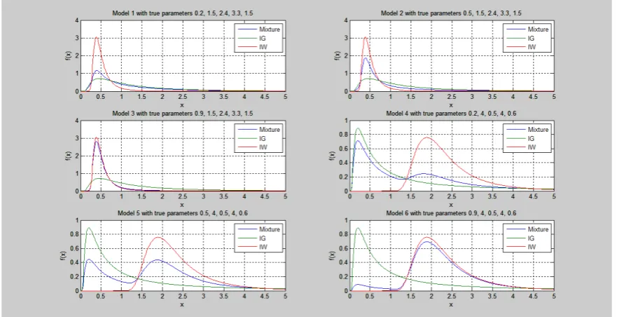
In this paper six different models are taken into account representing various shapes of the mixture. Thus if
(p, μ, α, β, λ) is a vector of the mixture parameters, then the models considered have the following values: (0.2, 1.5, 2.4, 3.3, 1.5), (0.5, 1.5, 2.4, 3.3, 1.5), (0.9, 1.5, 2.4, 3.3, 1.5), (0.2, 4.0, 0.5, 4.0, 0.6), (0.5, 4.0, 0.5, 4.0, 0.6), and (0.9, 4.0, 0.5, 4.0, 0.6). Figure 1 shows these six different cases respectively.
Gaussian – Inverse Weibull Mixture Model / IJMA- 5(3), March-2014.
3. MAXIMIUMLIKELIHOOD APPROCH
The maximum likelihood estimation for the parameters of a mixture of distributions has been studied extensively. Hasselblad [11] was one of the first researchers who used the maximum likelihood estimationfor mixtures of two or more components from exponential family. Generally speaking, applying the maximum likelihood method to mixtures involves using numerical iterative technique to find a solution and applying the expectation maximization (EM) algorithm. Hence this finds approximate values for the parameters.
Let L be the likelihood function and L* be the log-likelihood function, then differentiating L* with respect to the five parameters (p, μ, α, β, λ) of the mixture gives:
g1=∂L ∗
∂p = �
f1(xi) − f2(xi)
f(xi) (7) n
i=1
g2= ∂L ∗
∂μ = � 1
f(xi) (1 − p)
∂f2(xi)
∂μ
n
i=1
(8)
g3=∂L ∗
∂α = � 1 f(xi) n
i=1
p ∂f1∂α (9) (xi)
g4= ∂L ∗
∂β = � 1 f(xi) p
∂f1(xi)
∂β
n
i=1
(10)
g5= ∂L ∗
∂ λ = � 1
f(xi) (1 − p )
∂f2(xi)
∂λ
n
i=1
(11)
Solving the previous system of nonlinear equations in the five parameters gives estimators for those parameters. This of course involves more details that can be summarized in the following steps:
a. Generate 10000 samples of sizes 30, 50, 70, 90 for every model of the six models representing various shapes of the mixture distribution ft.
b. Estimate the five parameters for each sample in (a)
c. Find the integrated square error ISEmle = ∫(ft − fmle )2dx between the model used for generating the sample f and the model with estimated parameters fmle.
d. Compute the mean integrated square error MSEmle for the 10000 runs from each sample size with the corresponding standard deviation.
3. NON-PARAMETRIC DENSITY BASED APPROACH
In this section the proposed method of parameter estimation for the mixture model under study will be surveyed. The method is a modification of the general minimum distance estimation (MDE). The method is based on finding the parameters of the distribution that makes the distance between the distribution and the empirical distribution function minimum. MDE uses a goodness of fit statistic as the function to be minimized over the parameters space which consists of five components(p, μ, α, β, λ). Among these goodness of fit statistics are chi-square statistic, Cramer-von-Mises statistic, Kolmogorov Smirnov statistic, and Anderson Darling statistic.Hobbs et. al. [12] used the MDE method for the three parameter Weibull distribution. Sultan [13] described a method for the estimation of the three-parameter Weibull distribution function from censored samples. In the current research paper Cramer-von-Mises statistic is to be used. This statistic has the form:
W2= n � �F
t(x) − F�(x)� 2
dF0(x) ∞
−∞
` (12)
where F�(x) is the empirical distribution function and Ft(x) is the cumulative distribution function of the underlying distribution. A computational form is:
W2= � �F
t(xi) −i − 0.5n � 2 n
i=1
+12n (13)1
F�(x) = �nh �1 1
√2πexp �−
1 2 �
x − Xi
h �
2
�
n
i=1
dx
x
−∞
=1n � � 1
√2πhexp �− 1 2 �
x − Xi
h �
2
� dx
x
−∞ n
i=1
=1n� ∅ �x − Xh � i (14)
n
i=1
where ∅(x) is the cumulative distribution function of the standard normal distribution. Hence W2 takes the form:
W2= � �F
t�xj� −1n � ∅ �Xj− Xh �i n
i=1
�
2 n
j=1
+12n (15)1
with h as the window width of the kernel. The optimal value of the h parameter is:
hopt =2√π1 �� ft′′ 2
(x)dx�
−1 5
n−15 (16)
This form depends on finding ft′′(x) which is unknown. An empirical choice of h = sn−15 with s as the sample standard deviation proved to work well.
Estimating the parameters when using a nonparametric density estimator for the mixture can be summarized in the following steps:
1. Choose the sample size (sample sizes used here are 30, 50, 70, 90) and choose a model by defining the values for the parameters (p, μ, α, β, λ) from the six models considered.
2. Generate 10000 different samples from the true density of the chosen model ft for the chosen sample size. 3. Optimize W2 over the space of the unknown five parameters of the model. This gives an estimator fCvM of the
true density ft.
4. Compute the integrated square error measuring the distance between the true density and the estimated one as:
ISECvM = �(ft − fCvM )2dx (17)
then compute the mean integrated square error for the 10000 samples generated and denote it as MISECvM together with the corresponding standard deviation.
5. Similarly the mean integrated square error associated with maximum likelihood estimator is found.
4. RESULTS AND CONCLUSIONS
The following are the results of estimating the parameters of the distribution of the mixture model with five parameters
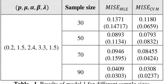
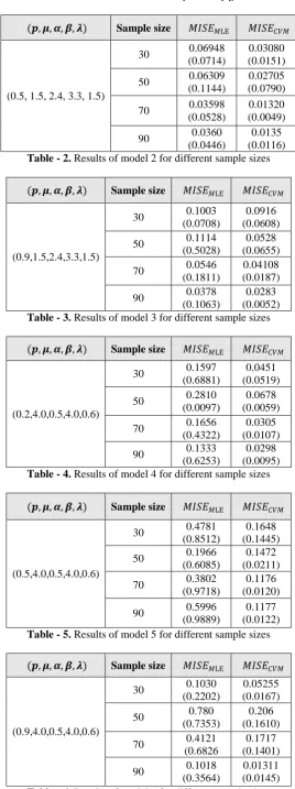
(p, μ, α, β, λ) for samples of different sizes 30, 50, 70, 90 to cover the spectrum of various shapes of the mixture mentioned above. Both the MLE and the proposed MDE are considered and results are given in table 1 to table 6 for
MISEMLE and MISECvM with the corresponding standard deviation between brackets for the 6 models respectively.
𝑀𝑀𝑀𝑀𝑀𝑀𝑀𝑀CV 𝑀𝑀
𝑀𝑀𝑀𝑀𝑀𝑀𝑀𝑀𝑀𝑀LE Sample size
(𝒑𝒑, 𝝁𝝁, 𝜶𝜶, 𝜷𝜷, 𝝀𝝀)
0.1180 (0.0659) 0.1371
(0.14717) 30
(0.2, 1.5, 2.4, 3.3, 1.5)
0.0793 (0.0832) 0.0893
(0.1134) 50
0.08455 (0.0424) 0.0946
(0.1595) 70
0.0308 (0.0237) 0.0409
(0.0303) 90
Gaussian – Inverse Weibull Mixture Model / IJMA- 5(3), March-2014.
𝑀𝑀𝑀𝑀𝑀𝑀𝑀𝑀𝐶𝐶𝐶𝐶𝑀𝑀 𝑀𝑀𝑀𝑀𝑀𝑀𝑀𝑀𝑀𝑀LE
Sample size
(𝒑𝒑, 𝝁𝝁, 𝜶𝜶, 𝜷𝜷, 𝝀𝝀)
0.03080 (0.0151) 0.06948
(0.0714) 30
(0.5, 1.5, 2.4, 3.3, 1.5)
0.02705 (0.0790) 0.06309 (0.1144) 50 0.01320 (0.0049) 0.03598 (0.0528) 70 0.0135 (0.0116) 0.0360 (0.0446) 90
Table - 2. Results of model 2 for different sample sizes
𝑀𝑀𝑀𝑀𝑀𝑀𝑀𝑀𝐶𝐶𝐶𝐶𝑀𝑀 𝑀𝑀𝑀𝑀𝑀𝑀𝑀𝑀𝑀𝑀LE
Sample size
(𝒑𝒑, 𝝁𝝁, 𝜶𝜶, 𝜷𝜷, 𝝀𝝀)
0.0916 (0.0608) 0.1003 (0.0708) 30 (0.9,1.5,2.4,3.3,1.5) 0.0528 (0.0655) 0.1114 (0.5028) 50 0.04108 (0.0187) 0.0546 (0.1811) 70 0.0283 (0.0052) 0.0378 (0.1063) 90
Table - 3. Results of model 3 for different sample sizes
𝑀𝑀𝑀𝑀𝑀𝑀𝑀𝑀𝐶𝐶𝐶𝐶𝑀𝑀 𝑀𝑀𝑀𝑀𝑀𝑀𝑀𝑀𝑀𝑀LE
Sample size
(𝒑𝒑, 𝝁𝝁, 𝜶𝜶, 𝜷𝜷, 𝝀𝝀)
0.0451 (0.0519) 0.1597 (0.6881) 30 (0.2,4.0,0.5,4.0,0.6) 0.0678 (0.0059) 0.2810 (0.0097) 50 0.0305 (0.0107) 0.1656 (0.4322) 70 0.0298 (0.0095) 0.1333 (0.6253) 90
Table - 4. Results of model 4 for different sample sizes
𝑀𝑀𝑀𝑀𝑀𝑀𝑀𝑀𝐶𝐶𝐶𝐶𝑀𝑀 𝑀𝑀𝑀𝑀𝑀𝑀𝑀𝑀𝑀𝑀LE
Sample size
(𝒑𝒑, 𝝁𝝁, 𝜶𝜶, 𝜷𝜷, 𝝀𝝀)
0.1648 (0.1445) 0.4781 (0.8512) 30 (0.5,4.0,0.5,4.0,0.6) 0.1472 (0.0211) 0.1966 (0.6085) 50 0.1176 (0.0120) 0.3802 (0.9718) 70 0.1177 (0.0122) 0.5996 (0.9889) 90
Table - 5. Results of model 5 for different sample sizes
𝑀𝑀𝑀𝑀𝑀𝑀𝑀𝑀𝐶𝐶𝐶𝐶𝑀𝑀 𝑀𝑀𝑀𝑀𝑀𝑀𝑀𝑀𝑀𝑀LE
Sample size
(𝒑𝒑, 𝝁𝝁, 𝜶𝜶, 𝜷𝜷, 𝝀𝝀)
0.05255 (0.0167) 0.1030 (0.2202) 30 (0.9,4.0,0.5,4.0,0.6) 0.206 (0.1610) 0.780 (0.7353) 50 0.1717 (0.1401) 0.4121 (0.6826 70 0.01311 (0.0145) 0.1018 (0.3564) 90
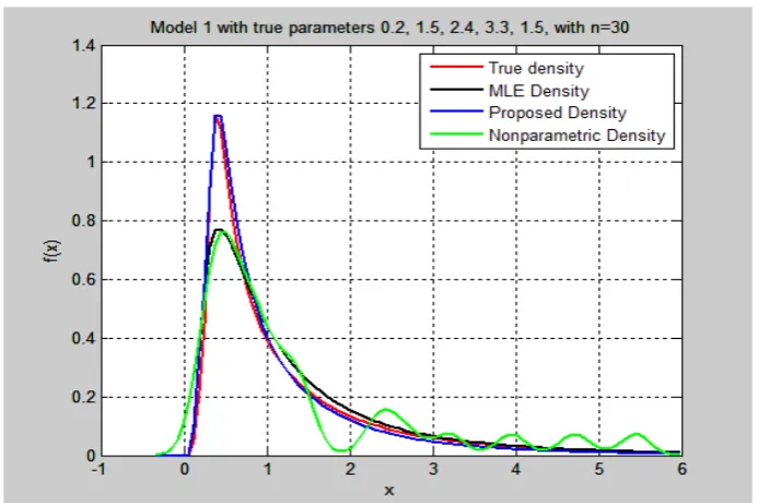
The above results show a better performance of the proposed method over the MLE method. The following tables (Table 7 To Table 12) give examples for a sample size of 30 for the six models considered. Each table shows sample points and the estimators for the MLE and the proposed method together with the true parameters. The integrated square error for both ME and the proposed method denoted by 𝑀𝑀𝑀𝑀𝑀𝑀𝑀𝑀𝑀𝑀𝑀𝑀 and 𝑀𝑀𝑀𝑀𝑀𝑀𝐶𝐶𝐶𝐶𝑀𝑀 respectively. Figure 2 to Figure 7 show the corresponding densities from tables.
Table - 7. A case for sample size of 30 from model 1
Fig. - 2: Estimated densities for case in Table 7.
Table - 8. A case for sample size of 30 from model 2
1.23 0.32 0.59 0.51 0.95 2.69 0.76 0.33 0.30 1.01 0.43 0.88 0.37 2.43 3.95 5.44 1.42 0.44 0.81 1.34 2.31 0.57 3.20 1.09 0.23 0.62 0.45 4.71 0.76 1.42 Sample
(𝑛𝑛 = 30)
𝑀𝑀𝑀𝑀𝑀𝑀𝐶𝐶𝐶𝐶𝑀𝑀
𝑀𝑀𝑀𝑀𝑀𝑀𝑀𝑀𝑀𝑀𝑀𝑀
Proposed method MLE
True Parameter
h =
0.
18
52
0.0049 0.0284
0.180 0.0006
0.2 𝑝𝑝
1.232 1.385
1.5 𝜇𝜇
2.230 1.501
2.4 𝛼𝛼
3.120 2.350
3.3 𝛽𝛽
1.330 1.381
1.5 𝜆𝜆
0.41 0.61 0.63 0.36 1.19 1.08 1.33 0.66 1.42 0.84 0.18 0.40 0.29 0.33 1.88 0.28 1.91 0.58 0.44 0.33 1.99 0.30 0.34 0.34 0.58 0.47 0.63 0.60 0.54 3.42 Sample
(𝑛𝑛 = 30)
𝑀𝑀𝑀𝑀𝑀𝑀𝐶𝐶𝐶𝐶𝑀𝑀
𝑀𝑀𝑀𝑀𝑀𝑀𝑀𝑀𝑀𝑀𝑀𝑀
Proposed method MLE
True Parameter
h =
0.
09
16
0.0083 0.0539
0.576 0.617
0.5 𝑝𝑝
1.229 1.206
1.5 𝜇𝜇
2.230 2.527
2.4 𝛼𝛼
2.942 2.259
3.3 𝛽𝛽
1.114 1.475
Gaussian – Inverse Weibull Mixture Model / IJMA- 5(3), March-2014.
Fig. - 3: Estimated densities for case in Table 8.
Table - 9. A case for sample size of 30 from model 3
Fig. - 4: Estimated densities for case in Table 9.
0.33 0.75 0.81 0.72 0.45 0.40 0.48 0.56 0.12 0.58 0.92 0.35 1.56 0.32 0.41 0.59 0.45 0.38 0.35 0.34 0.69 0.34 0.28 0.33 1.45 0.31 0.87 0.50 0.43 0.55 Sample
(𝑛𝑛 = 30)
𝑀𝑀𝑀𝑀𝑀𝑀𝐶𝐶𝐶𝐶𝑀𝑀
𝑀𝑀𝑀𝑀𝑀𝑀𝑀𝑀𝑀𝑀𝑀𝑀
Proposed method MLE
True Parameter
h =
0.
48
0.0036 0.0143
0.933 0.890
0.9 𝑝𝑝
1.164 1.054
1.5 𝜇𝜇
2.398 2.431
2.4 𝛼𝛼
3.355 3.588
3.3 𝛽𝛽
0.516 0.308
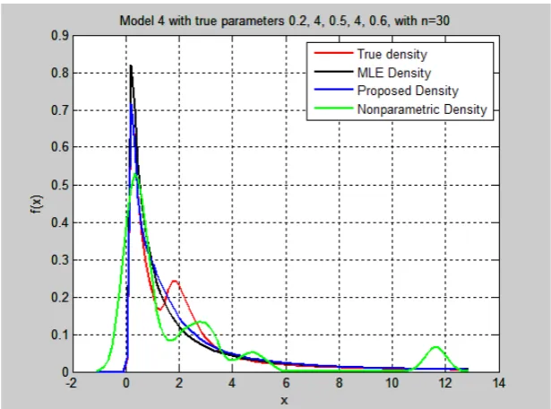
Table - 10. A case for sample size of 30 from model 4
Fig. - 5: Estimated densities for case in Table 10.
Table - 11. A case for sample size of 30 from model 5
0.12 0.26 0.32 1.17 0.19 4.45 0.39 2.69 0.37 2.25 2.99 0.24 5.04 0.24 3.11 0.69 11.60 0.15 0.18 0.44 2.29 0.45 11.66 0.30 1.04 3.26 0.39 1.88 0.67 0.58 Sample
(𝑛𝑛 = 30)
𝑀𝑀𝑀𝑀𝑀𝑀𝐶𝐶𝐶𝐶𝑀𝑀
𝑀𝑀𝑀𝑀𝑀𝑀𝑀𝑀𝑀𝑀𝑀𝑀
Proposed method MLE
True Parameter
h =
0.
30
71
0.0089 0.0173
0.244 0.120
0.2 𝑝𝑝
3.135 3.065
4.0 𝜇𝜇
0.593 0.644
0.5 𝛼𝛼
1.525 1.280
4.0 𝛽𝛽
0.582 0.597
0.6 𝜆𝜆
2.46 0.12 1.65 1.17 3.04 0.63 1.85 0.41 0.18 2.30 2.48 2.03 0.39 2.06 11.58 1.94 3.85 0.23 3.06 0.11 2.68 2.48 0.63 1.57 1.29 3.35 2.03 1.71 0.30 2.26 Sample
(𝑛𝑛 = 30)
𝑀𝑀𝑀𝑀𝑀𝑀𝐶𝐶𝐶𝐶𝑀𝑀
𝑀𝑀𝑀𝑀𝑀𝑀𝑀𝑀𝑀𝑀𝑀𝑀
Proposed method MLE
True Parameter
h =
0.
18
61
0.0043 0.0298
0.624 0.604
0.5 𝑝𝑝
1.567 1.565
4.0 𝜇𝜇
0.488 0.563
0.5 𝛼𝛼
3.203 2.864
4.0 𝛽𝛽
0.707 0.812
Gaussian – Inverse Weibull Mixture Model / IJMA- 5(3), March-2014.
Fig. - 6: Estimated densities for case in Table 11.
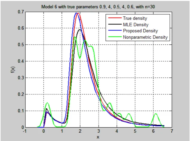
Table - 12. A case for sample size of 30 from model 6
Fig. - 7: Estimated densities for case in Table 12.
1.93 2.64 2.79 1.71 6.13 1.67 3.69 4.66 2.21 2.48 3.17 2.17 2.59 4.14 2.17 2.52 2.33 0.13 1.61 3.53 2.31 2.91 0.28 2.15 1.68 1.62 2.70 1.87 1.77 2.85 Sample
(𝑛𝑛 = 30)
𝑀𝑀𝑀𝑀𝑀𝑀𝐶𝐶𝐶𝐶𝑀𝑀
𝑀𝑀𝑀𝑀𝑀𝑀𝑀𝑀𝑀𝑀𝑀𝑀
Proposed method MLE
True Parameter
h =
0.
30
71
0.0088 0.093
0.903 0.896
0.9 𝑝𝑝
4.025 3.888
4.0 𝜇𝜇
0.523 0.473
0.5 𝛼𝛼
3.797 3.610
4.0 𝛽𝛽
0.538 0.474
5. REFERENCES
1.
J. Fonseca, The Application of Mixture Modeling and Information Criteria for Discovering Patterns of Coronary Heart Disease, Journal of Applied Quantitative Methods, 3, 292-302, 20082.
G. Mclachlan and K. Basford, Mixture Models Inference and Applications to Clustering, Marcel Dekker, New York, 1988.3.
C. Priebe, Adaptive Mixtures , American Statistical Association, 89 ,796-806, 1994.4.
C. Bishop, Neural Networks for Pattern Recognition, Oxford University Press Link, Oxford, 1995.5.
A. Dempster; N. Laird; and D. Rubin, Maximum Likelihood from Incomplete Data via the EM Algorithm,Journal of the Royal Statistical Society, 39, 1-38, 1977.
6.
G. Mclachlan, The Em Algorithm and Extensions, Wiley and Sons, New York, 1997.7.
Z. Keller and R. Kmath, Reliability Analysis of CNC Machine Tools, Reliability Engineering, 3, 449-473, 1982.8.
P. Pawlas and D. Szynal Characterizations of the inverse Weibull distribution and generalized extreme value distributions ny moments of Kth record values, Applicationes Mathematicae, 27,2 , 197–202, 2000.9.
P. Erto, Genesis, properties and identification of the inverse Weibull lifetime model, Statistica Applicata, 1, 117-128, 1989.10.
N. Johnson; and S. Kotz, Distributions in Statistics: Continuous Univariate Distributions, Wiley and sons, New York, 1970.11.
V. Hasselblad, Estimation of Finite Mixture of Distributions from the Exponential Family, Journal of the American Statistical Association, 64, 1459-1471, 1969.12.
R, Hobbs; A. Moore; and R. Miller, Minimum distance estimation of the three parameter Weibull distribution,IEEE Transaction in Reliability, 5, 459-469, 1985