Neuron, Volume
102
Supplemental Information
Discrete Stepping and Nonlinear Ramping Dynamics
Underlie Spiking Responses of LIP Neurons
during Decision-Making
David M. Zoltowski, Kenneth W. Latimer, Jacob L. Yates, Alexander C. Huk, and Jonathan
W. Pillow
+high +low zero
-low
-high
200 700
population
time (ms)
step +history linear +history linear +b, +history sqrt +b, +history
200 700 200 700200 700 200 700
200 700
time (ms) firing rate (sp/s) 5
30
200 700
5 30
200 700200 700 200 700
B
A
-.010 0 >.02 5
10
-.010 0 >.02 5
10
+low - -low
+low - -low
in-RF out-RF
# of cells
in-RF out-RF
<-.02 00 >.04 5
10 15
<-.020 0 .01 5
10
-high - -low
+high - +low
variance
5 30
C
fraction hit upper boundary
# of cells
in-RF in-RF, +high
0 0.5 1
0 10 20
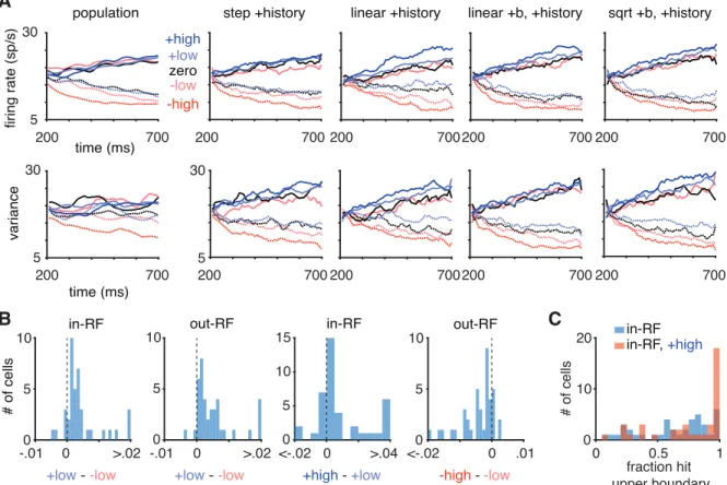
Figure S1. Choice-conditioned analyses, related to Figure2. A.Left: the PSTH and spike count variance conditioned on in-RF (solid lines) and out-RF (dashed line) choices, averaged across all cells. Right: simu-lated PSTHs and spike count variances conditioned on choice from the models using the inferred parameters for each cell. For the stepping model, we simulated choices based on the simulated step direction. The probability of an in-RF choice was 0.99, 0.01, and 0.5 given a step to the up state↵2, down state↵1, no step during the trial, respecitvely. In the ramping models, the probability of an in-RF choice was computed using a sigmoid function asp(in-RF choice) = 1+exp( k1(xT x0)), wherexT was the value of the latent trajectory at the end of the trial,x0was the inferred mean diffusion start location parameter in the ramping model, and
k = 5. We thresholdedx0to be in the range [0.1,0.9]. B.We computed the posterior mean of the latent
ramping trajectoriesx1:T for each trial to test whether the motion coherence had an effect on the firing rate for trials with the same choice. We computed the average latent ramping slope during the first200ms of each trial for +low and -low coherence trials, separated by choice. The +low coherence trials had more positive slopes than -low coherence trials on both in-RF (p = 0.0059, one-sided paired t-test) and out-RF choice trials (p= 0.0024, one-sided paired t-test). The +high coherence trials had more positive slopes than +low coherence trials on in-RF choice trials (p= 0.0042, one-sided paired t-test), while the -high coherence trials had more negative slopes than -low coherence trials on out-RF choice trials (p= 1.03e 5, one-sided paired t-test). C.The distribution across cells of the fraction of trials for which the median of the posterior over the ramping bound-hit time was before the analysis window ended for in-RF and in-RF, +high trials.
ΔWAIC (55/60 correct)
ΔDIC (26/60 correct)
0 60
-600 0 600
Δ firing rate
D
E
Cell ΔW
AIC
ramp +history
A
true ramp +history true step +history
step +history
-500 0 100
-100 0 500
ramp +b, +history
true ramp +b, +history true step +history
step +history
B
0 100
<-100 0 >100
Δ firing rate
ΔWAIC (74/80 correct)
ΔDIC (45/80 correct) single coherence simulations without history
Cell ΔW
AIC
ΔWAIC ΔDIC correct
ΔWAIC ΔDIC -500
0 100
-100 0 500
single coherence simulations with history
C
Cell ΔW
AIC
-500 0 100
-1000 500
true sqrt +b, +history true step +history
sqrt +b, +history step +history
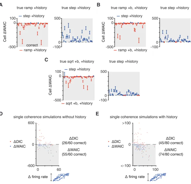
Figure S2. The WAIC correctly identifies simulated data from different models, related to Figures4and5.
A.The WAIC reliably distinguished data from the ramping and stepping models with spike-history simulated from the mean parameters of the ramping (left) and stepping (right) models with spike-history for each cell. The number of simulated trials per motion coherence was matched to the true number for each cell. B.
Same asA, except with ramping with non-zero baseline and history model. C.Same asA-B, except with the square root ramping with non-zero baseline and history model. D.-E. Model comparison results from simulated single-coherence ramping data as a function of the change in firing rate from the beginning to the end of the trial using the DIC and WAIC. The WAIC correctly identifies data simulated from single-coherence ramping models (Chandrasekaran et al.,2016).
A
B
random onset & offset (1)
0 2 4 0
3 6
0 20 40
0 3 6 random onset & offset (2) random offset
random onset (2)
-80 -40 0 40 80 -80 -40 0 40 80
0 3 6
# simulations
firing rate (sp/s)
200 1200
time (ms)
200 1200
time (ms) 0
20 40
firing rate (sp/s)
0 20 40
firing rate (sp/s)
0 20 40
firing rate (sp/s)
0 20 40
firing rate (sp/s)
0 2 4
ΔWAIC ΔWAIC
-80 -40 0 40 80 -80 -40 0 40 80 200 1200
time (ms)
200 1200
time (ms) ΔWAIC ΔWAIC
-80 -40 0 40 80
200 1200
time (ms) ΔWAIC
# simulations
# simulations # simulations
# simulations
random onset (1)
C
D
E
ramp step
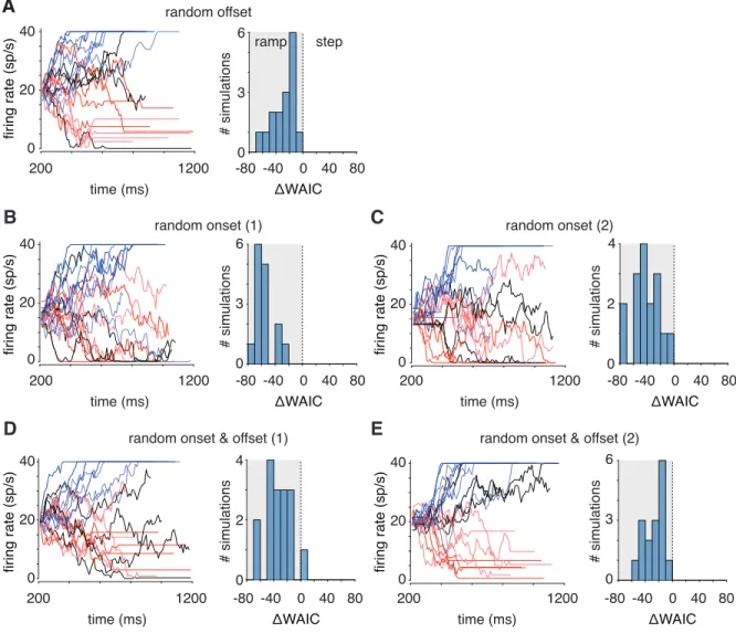
Figure S3. Simulated model comparison between the stepping model with history and the linear ramping model with history with random integration onset and/or offset times, related to Figures4and 5. A. Left: Example simulated firing rates from the ramping model with history with a random integration offset time. On each trial, the offset time was set to100ms after a competing accumulator with perfectly anticorrelated diffusion noise hit the upper boundary (Mazurek et al.,2003;Latimer et al.,2017). Right: WAIC differences between the ramping and stepping models with history fit to 16 simulated cells. Positive values favor the step-ping model with history.B.Same asA, except for with a random integration onset time on each trial that was set to200ms plus10ms times a sample from a negative binomial distribution. Here, the parameters of the negative binomial distribution werer= 1.2andp= 0.4, which generated integration onset times with mean 207.9ms and std11.2ms.C.Same asB, except with onset times simulated from a negative binomial distri-bution with parametersr= 1.4andp= 0.8, which generated onset times with mean255.2ms and std52.2 ms.D-E.Same asA, except with both random integration onset and offset times. The integration onset times were generated from the distributions inBandC, respectively. In all but one simulation, the WAIC favored the ramping model with history. For all simulations, we set the following ramping with history model parameters to
cell
21 28 12
5
linear +history step +history
-150 -100 -50 0 50 100
Cell ΔLOO
cell cell
14 21
1910
13 16
2413
linear +b, +history sqrt +b, +history
-200 -150 -100 -50 0 50 100
-200 -150 -100 -50 0 50 100
A
C
B
linear +history step +history
-0.4 -0.2 0 0.2 0.4 0.6
-high -low zer
o +low +high out-RF in-RF
coherence choice
mean trial ΔLOO
step +history
Cell ΔLOO
-0.2 0 0.2
fit zer o
fit +cohfit in-RF
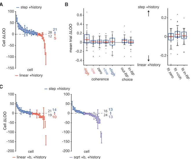
Figure S4. Model comparison using leave-one-out cross validation, related to Figures 4and5. We used PSIS-LOO to estimate the Bayesian leave-one-out cross validation performance (LOO) on held out trials
(Ve-htari et al.,2017). In Bayesian LOO, predictive performance on a held-out trial is evaluated by integrating over
the posterior distribution of the parameters conditioned on the rest of the trials. PSIS-LOO uses importance sampling to estimate this integral. The proposal distribution is the posterior distribution conditioned on all of the trials (which we sample from in our MCMC procedure) and the importance weights are stabilized through regularization. Model comparison using LOO provided nearly identical results to the model comparison using WAIC.A.Sorted LOO differences between the stepping and linear ramping models with spike-history for all neurons (error bars indicate±1SEM). Color conventions are the same as in Figure4. B. Left: Mean LOO differences across trials of each motion coherence or choice. Right: Mean LOO differences across trials computed for models fit only to data from zero coherence, positive coherence, or in-RF trials (respectively).
C.Sorted LOO differences between the stepping model and the linear (left) and sqrt (right) ramping models with non-zero baseline and spike-history for all cells.
3 3.5 0
2 4
3 3.2 3.4 0
2 4
3 3.2 3.4 0
2 4
2 2.2 2.4 0
5
1.5 2 2.5 0
2 4
2 2.2 2.4 0
2 4
1.6 1.8 2 0
5
1.6 1.8 2 0
2 4
1.7 1.8 1.9 0
2 4
3.8 4 4.2 0
2 4
3.8 3.9 4 0
2 4
3.8 4 4.2 0
2 4
step +history
linear +history linear +b, +history
frequency
WAIC [x104]
Cell 1
Cell 2
Cell 3
Cell 4
simulated data
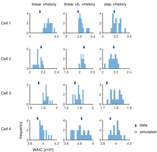
Figure S5. Comparison of WAIC values fit to simulated data and WAIC values for the experimental data, related to Figures4and5. For four different cells, we simulated 16 synthetic datasets each from the inferred parameters of the linear ramping with zero baseline, linear ramping with non-zero baseline, and stepping models (all with history). We then fit the corresponding model to each simulated dataset and computed the WAIC of the simulated data given the true model (light blue histograms). We compared these values with the WAIC values computed on the experimental data (dark blue arrow). For the linear ramping with non-zero baseline and stepping models with history, the WAIC values of the true data were most often within the range of WAIC values computed on simulated data. For this analysis, we selected two of the cells with the strongest choice selectivity (cells 1 and 2) and two random cells (cells 3 and 4).
0 10 20 30 40 50 mean firing rate (sp/s)
-0.8 -0.6 -0.4 -0.2 0 0.2 0.4
normalized W
AIC dif
fer
ence
zero baseline nonzero baseline
B
A
0 10 20 30 40
in-RF - out-RF (sp/s) -0.6
-0.3 0.3
normalized W
AIC dif
ference
0
Figure S6. Relationship between WAIC differences and firing rates, related to Figure4. A-B.For each cell, the average WAIC difference across trial is plotted against (A) the overall mean firing rate for that cell and (B) the difference in firing rates at the end of in-RF vs. out-RF trials for that cell. The different color dots correspond to comparison of the (red) linear ramping model with zero baseline and history and (blue) linear ramping model with baseline and history against the stepping model with history, respectively. The correlation between the mean firing rate and the normalized WAIC differences is weak (⇢= 0.01and⇢= 0.15for the zero baseline and nonzero baseline conditions, respectively). The data exhibit negative correlations between the modulation in firing rate across the in-RF and out-RF conditions and the WAIC differences (⇢ = 0.35 and⇢= 0.52for the zero baseline and nonzero baseline conditions, respectively).
0 >1000
Cell ΔW
AIC
B
C
7 8 8
2
3 8 8
6
2 8 8 6
+b +b
+history sqrt quad exp
linear reaction time task
Cell ΔW
AIC
-60 0 80
-80 0 40
-80 0 40
cell step +history
linear +history
linear +b, +history
sqrt +b, +history
population PSTH step +history linear +history linear +b, +history sqrt +b, +history
200 600
20 70
firing rate (sp/s)
+high +low zero -low -high
200 600 200 600 200 600 200 600
A
time (ms)
Figure S7. Analysis of LIP responses (N = 16) in a reaction-time (RT) task (Roitman and Shadlen,2002), related to Figure7. A. Population PSTH and simulated PSTHs from the fitted models, aligned to motion onset.B.Model comparison of extended ramping models and linear ramping model. Including spike-history dependence and non-zero baseline firing rates improved ramping model performance but different nonlin-earities performed similarly. C. Comparison of the stepping model and different ramping models, all with spike-history. See FigureS8for a comparable analysis using cross-validation.
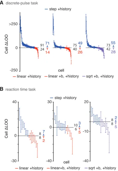
reaction time task discrete-pulse task
A
B
-250 0 >250
Cell ΔLOO
cell
step +history
linear +history linear +b, +history sqrt +b, +history
-30 0 40
-40 0 30
-40 -10 20
7
8 8 2
3
10 6 5
2
8 8
5
Cell ΔLOO
cell
step +history
linear +history linear+b, +history sqrt +b, +history 71
91 24
14
49
75 40
26
55
73 42
28
Figure S8.Model comparison using leave-one-out cross validation (LOO) for the (A) discrete-pulse and (B) reaction time data, related to Figures7andS7. LOO was estimated using PSIS-LOO (Vehtari et al.,2017, see FigureS4). Model comparison using LOO for these datasets provided similar results to model comparison using WAIC.