STATIC ANALYSIS OF TENSEGRITY STRUCTURES

(1)

By

JULIO CESAR CORREA

A THESIS PRESENTED TO THE GRADUATE SCHOOL OF THE UNIVERSITY OF FLORIDA IN PARTIAL FULFILLMENT

OF THE REQUIREMENTS FOR THE DEGREE OF MASTER OF SCIENCE

UNIVERSITY OF FLORIDA 2001

(2)

(3)

iii

ACKNOWLEDGMENTS

I want to thank to Dr. Carl Crane and Dr. Ali Seirig, members of my committee for their overseeing of the thesis and for their valuable suggestions.

My special thanks go to Dr. Joseph Duffy, my committee chairman, for showing confidence in my work, and for his support and dedication. More than academic knowledge I have learned from him that wisdom and simplicity go together.

(4)

iv

TABLE OF CONTENTS

page

ACKNOWLEDGMENTS ...iii

ABSTRACT... vi

CHAPTERS 1 INTRODUCTION ... 1

2 BASIC CONCEPTS ... 4

2.1 The Principle of Virtual Work...4

2.2 Plücker Coordinates ...8

2.3 Transformation Matrices...11

2.4 Reaction Forces and Reaction Moments ...16

2.5 Numerical Example ...18

2.6 Verification of the Numerical Results...30

3 GENERAL EQUATIONS FOR THE STATICS OF TENSEGRITY STRUCTURES... 34

3.1 Generalized Coordinates...37

3.2 The Principle of Virtual Work for Tensegrity Structures...38

3.3 Coordinates of the Ends of the Struts...40

3.4 Initial Conditions...42

3.5 The Virtual Work Due to the External Forces ...47

3.6 The Virtual Work Due to the External Moments ...49

3.7 The Potential Energy...50

3.8 The General Equations ...52

4 NUMERICAL RESULTS ... 56

4.1 Analysis of Tensegrity Structures in their Unloaded Positions ...56

4.2 Analysis of Loaded Tensegrity Structures ...58

4.3 Example 1: Analysis of a Tensegrity Structure with 3 Struts ...64

4.3.1 Analysis for the Unloaded Position...64

(5)

v

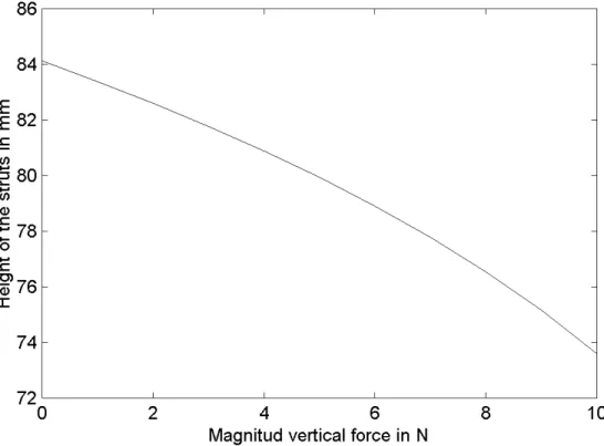
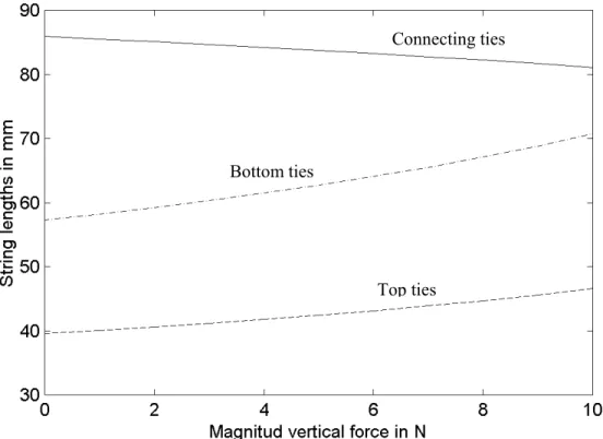
4.4.2 Analysis for the Loaded Position ...81

4.5.2 Analysis for the Loaded Position ...94

5 CONCLUSIONS ... 101

APPENDICES A FIRST EQUILIBRIUM EQUATION FOR THE STATICS OF A TENSEGRITY STRUCTURE WITH 3 STRUTS ... 104

B SOFTWARE FOR THE STATIC ANALYSIS OF A TENSEGRITY STRUCTURE... 105

REFERENCES ... 107

(6)

vi

Abstract of Thesis Presented to the Graduate School of the University of Florida in Partial Fulfillment of the Requirements for the Degree of Master of Science STATIC ANALYSIS OF TENSEGRITY STRUCTURES

By

Julio César Correa August 2001 Chairman: Dr. Joseph Duffy

Major Department: Mechanical Engineering

Tensegrity structures are three dimensional assemblages formed of rigid and elastic elements. They hold the promise of novel applications. However their behavior is not completely understood at this time. This research addresses the static analysis problem and determines the position assumed by the structure when external loads are applied. The derivation of the mathematical model for the equilibrium positions of the structure is based on the virtual work principle together with concepts related to geometry of lines. The solution for the resultant equations is performed using numerical methods. Several examples are presented to demonstrate this approach and all the results are carefully verified. A software that is able to generate and to solve the equilibrium equations is developed. The software also permits one to visualize different equilibrium positions for the analyzed structure and in this way to gain insight in the physics and the geometry of tensegrity systems.

(7)

1

CHAPTER 1 INTRODUCTION

Tensegrity structures are spatial structures formed by a combination of rigid elements (the struts) and elastic elements (the ties). No pair of struts touch and the end of each strut is connected to three non-coplanar ties [1].

The struts are always in compression and the ties in tension. The entire configuration stands by itself and maintains its form solely because of the internal arrangement of the ties and the struts [2].

Tensegrity is an abbreviation of tension and integrity. Figure 1.1 shows a number of anti-prism tensegrity structures formed with 3, 4 and 5 struts respectively.

Figure 1.1. Tensegrity structures conformed by 3, 4 and 5 struts.

The development of tensegrity structures is relatively new and the works related have only existed for the 25 years. Kenner [3] establishes the relation between the rotation of the top and bottom ties. Tobie [2] presents procedures for the generation of tensile structures by physical and graphical means. Yin [1]

(8)

obtains Kenner’s results using energy consideration and finds the equilibrium position for the unloaded tensegrity prisms. Stern [4] develops generic design equations to find the lengths of the struts and elastic ties needed to create a desired geometry. Since no external forces are considered his results are referred to the unload position of the structure. Knight [5] addresses the problem of stability of tensegrity structures for the design of a deployable antenna.

The problem of the determination of the equilibrium position of a tensegrity structure when external forces and external moments act on the structure has not been studied previously. This is the focus of this research.

It is known that when the systems can store potential energy, as in the case of the elastic ties of a tensegrity structure, the energy methods are applicable. For this reason the virtual work formulation was selected from several possible approaches to solve the current problem.

Despite their complexity, anti-prism tensegrity structures exhibit a pattern in their configuration. This fact is used to develop a consistent nomenclature valid for any structure and with this basis to develop the equilibrium equations. To simplify the derivation of a mathematical model some assumptions are included. Those simplifications are related basically with the absence of internal dissipative forces and with the number and fashion that external loads are applied to the struts of the structure.

Even for the simplest case the resultant equations are lengthy and highly coupled. Numerical methods offer an alternative to solve the equations. Parallel to the research presented here a software in Matlab was developed. Basically

(9)

the software is able to develop the equilibrium equations for a given tensegrity structure and to solve them when the external loads are given. The software uses the well known Newton Raphson method which is implemented by the function fsolve of Matlab. To avoid the limitations of numerical methods to converge to an answer, the proper selection of the initial conditions was considered carefully together with the guidance of the solution through small increments of the external loads.

Once the equations are solved, the output data consists of basically listing of the various coordinates of the ends of the structure expressed in a global coordinate system for the equilibrium position. When dealing with three dimensional systems, the numerical results by themselves are not sufficient to understand the behavior of the systems. To assist to the comprehension of the results the software developed provides graphic outputs. In this way the complex equilibrium equations are connected in an easy way to the physical situation.

One important question that arose was the validity of the numerical results. This point is specially important when one considers the complexity of the equations. An independent validation of the results was realized using Newton’s Third Law.

This thesis is basically as follows: Chapter 2 introduces the basic concepts related to the tools required to develop the mathematical model for a tensegrity structure, Chapter 3 develops a systematic nomenclature for the elements of a tensegrity structure and presents the mathematical model. Chapter 4 provides examples to illustrate the application of the model.

(10)

4 CHAPTER 2 BASIC CONCEPTS

The main objective of this research is to find the final equilibrium position of a general anti-prism tensegrity structure after an arbitrary load and or moment has been applied. In this chapter the main concepts involved in the derivations of the equations that govern the statics of the structure are presented.

2.1 The Principle of Virtual Work

The principle of virtual work for a system of rigid bodies for which there is no energy absorption at the points of interconnection establishes that the system will be in equilibrium if [6]

0

1

= ⋅

=

å

=

N

i

i r

F

W δ

δ (2.1)

where

:

W

δ virtual work.

: i

F force applied to the system at point i.

: i

r

δ virtual displacement of the vector ri. :

N number of applied forces.

The virtual displacement represents imaginary infinitesimal changes δri of

the position vector ri that are consistent with the constraints of the system but

(11)

of the instantaneous variations. The virtual displacements obey the rules of differential calculus.

If the system has p degrees of freedom there are p generalized coordinates q_k, k =1, 2, . . . , q_p, then the variation of ri must be evaluated

with respect to each generalized coordinate.

(

p

)

i

i r q q q

r = ₁, ₂, . . . ,

p p i i

i

i q

q r q

q r

r δ δ δ

δ

∂ ∂ + +

∂ ∂ + ∂

∂

= ₂ . . .

2 1

1

k k i p

k

i q

q r

r δ

δ

∂ ∂ =

å

=1

(2.2) The principle of virtual work can be modified to allow for the inclusion of internal conservative forces in terms of potential functions [6]. In general the virtual work includes the contribution of both conservative and non-conservative forces

c

nc W

W

W δ δ

δ = + (2.3)

where the subscripts nc and c denote conservative and non-conservative virtual work respectively.

The virtual work performed by the non-conservative forces can be expressed as

i nci

n

i

nc F r

W δ

δ .

1

å

₌

(12)

where Fnci is the non-conservative force i and n is the number of

non-conservative forces. Substituting (2.2) into (2.4) yields,

k k i nci n i p k

nc _q q

r F

W _δ

δ =

å

_∂∂

= = . 1 1 (2.5)

The virtual work performed by the conservative force j can be expressed in the form [7]

j

cj V

W δ

δ = − (2.6)

where V_j =V_j(q₁, q₂, . . . ,q_p) is the potential energy associated with the conservative force j. Therefore

÷ ÷ ø ö ç ç è æ ∂ ∂ + + ∂ ∂ + ∂ ∂ − = p p j j j

cj _q q

V q q V q q V

W δ δ δ

δ ₂ . . .

2 1

1

(2.7)

And the total virtual work performed by the conservative forces is given by

÷÷ø ö ççè æ ∂ ∂ −

=

å

=

= k k

j m

j p

k

c _q q

V W δ δ 1 1 (2.8)

where m is the number of conservative forces.

With the aid of (2.5) and (2.8), equation (2.3) can be rewritten in the form

k k j m j p k k i nci n i p k q q V q r F W δ δ ÷÷ø ö ççè æ ∂ ∂ − ∂ ∂ ⋅

=

å

= = =

=1 1 1 1

k k j m j k i nci n i p k q q V q r F δ ÷÷ø ö ççè æ ∂ ∂ − ∂ ∂ ⋅

=

å

= =

=1 1 1

(13)

The principle of virtual work requires that the preceding expression vanishes for the equilibrium. Because the generalized virtual displacements δq_k

are all independent and hence entirely arbitrary, (2.9) can be satisfied [7], if and only if

0 1

1

= ∂ ∂ −

∂ ∂

⋅

å

₌ ₌

k j m

j k

i nci n

i q

V q

r F

p k

q V Q

k j m

j

k 0, 1, 2, ,

1

L

= =

∂ ∂ −

å

=

(2.10)

where

k i nci

n

i k

q r F

Q

∂ ∂ ⋅ =

å

=1

(2.11) The term Q_k is known as the generalized forces and despite its name may include both the virtual work due to external non-conservative forces and the virtual work due to external non-conservative moments.

If the lower ends of the struts of a tensegrity system are constrained to move on the horizontal plane and also the rotation about the longitudinal axis of the strut is constrained, then each strut has 4 degrees of freedom and the whole system has

struts n

p=4* _ (2.12)

(14)

2.2 Plücker Coordinates

The coordinates of a line joining two finite points with coordinates )

, ,

(x₁ y₁ z₁ and (x₂,y₂,z₂) can be written as ú

û ù ê ë é

=

o

S S

$ (2.13)

where S is in the direction along the line and S0 is the moment of the line about the origin O. S and S0 can be evaluated from the coordinates of the points as follows [8]

ú ú ú û ù

ê ê ê ë é

=

N M L

S (2.14) where

2 1 1 1

x x

L = (2.15)

2 1 1 1

y y

M = (2.16)

2 1 1 1

z z

N = (2.17)

and

ú ú ú û ù ê ê ê ë é

=

R Q P

S_o (2.18) where

2 2

1 1

z y

P = (2.19)

2 2

1 1

x z

Q = (2.20)

2 2

1 1

y x

(15)

The numbers L, M, N, P, Q and R are called the Plücker line coordinates and they cannot be simultaneously equal to zero.

The Plücker line coordinates can be expressed in unitized form by dividing the vectors S and S0 by L2+M2 +N2 provided L, M and N are not all equal to zero.

ú û ù ê ë é

=

ú û ù ê ë é

+ + =

∧

o

o s

s S

S N M

L2 2 2

1

$ (2.22)

A force F can be expressed as a scalar multiple of the unit vector s

bound to the line. The moment of the force about a reference point O can be expressed as a scalar multiple of the moment vector s0 [9], therefore

ú û ù ê ë é

=

= ∧

o F

s s f f $

$ (2.23)

where f stands for the magnitude of the force F.

If L, M and N are all equal to zero the unitized Plücker line coordinates have the form

ú û ù ê ë é

=

ú û ù ê ë é

+ + =

∧

o

o s

S R Q P

0 0

1 $

2 2

2 (2.24)

And the Plücker line coordinates of a pure moment are

ú û ù ê ë é

=

= ∧

o M

s m

m $ 0

$ (2.25)

(16)

Consider two coordinates systems shown in Figure 2.1. The origin of system X'Y'Z' is translated by (x,y,z) and rotated arbitrarily with respect to system XYZ. The Plücker coordinates of the line $ expressed in the system

' ' 'Y Z

X can be transformed to the system XYZ using the following relation [9], $'

$ = e (2.26)

where

:

$ Plücker coordinates of the line expressed in the system XYZ

:

$' Plücker coordinates of the line expressed in the system X'Y'Z'

and

ú û ù ê

ë é

=

R R A

O R

e _A

B A B A B

3

3 _(2.27)

where :

R

A

B rotation matrix of the system X'Y'Z' with respect to the system XYZ

: 3

O zeroes 3x3 matrix

ú ú ú û ù ê

ê ê ë é

−

− − =

0 0 0 3

x y

x z

y z

A (2.28)

Conversely if the Plücker coordinates of the line are given in the system

' ' 'Y Z

X and it is desired to express them in the system XYZ, from (2.26) $

'

(17)

z

y

x

z' y'

x'

x

y

z $

Figure 2.1. General change of a coordinate system.

where

ú ú ú û ù ê

ê ê ë é

=

−

T A B T T A B

T A B

R A

R

O R

e

3 3

1 _(2.30)

2.3 Transformation Matrices

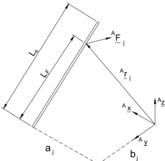
Figure 2.2 shows an arbitrary point P2 located on a strut of length L_s. In a reference system D whose z axis is along the axis of the strut and with its origin is located at the lower end of the strut, the coordinates of DP2 are simply (0,0,l). However frequently is more convenient for purposes of analysis to express the location of P2 in the global reference system A. This can be accomplished by a transformation matrix.

If the lower end of the strut is constrained to move on the horizontal plane )

(18)

can be modeled by an universal joint. In this way the joint provides the 4 degrees of freedom associated with the strut.

x

y

z

P

Po

_P

Ls l

r

A

D

1 2

Figure 2.2. Strut in an arbitrary position.

The alignment of the z axis on the fixed system with the axis of the rod can be accomplished using the following three consecutive transformations [10] :

Translation, t =(a,b,0), Figure 2.3. Note that the coordinate z is zero because of the restriction imposed to the movement of the lower end of the strut.

Rotation , about the current x axis (Bx), Figure 2.4. Rotation , about the current y axis (Cy_{), Figure 2.5.}

(19)

Figure 2.3. Translation (a,b,0) in the system A.

Figure 2.4. Rotation about xaxis in the Bsystem. z

B

y

B

x

B

z

A

y

A

x

A

a

b

t

z

C

z

A

x

A

y

A

y

C

y

B

x x C B _,

(20)

Figure 2.5. Rotation about current yaxis in the C system.

The coordinates of P2 measured in the global reference system are

2 0

, ,

2 T T T P

P C D

D B C b a A B A β ε

= (2.31)

where: ú ú ú ú û ù ê ê ê ê ë é = 1 0 0 0 0 1 0 0 0 1 0 0 0 1 0 , , b a T_a_b

A

B (2.32)

ú ú ú ú û ù ê ê ê ê ë é − = 1 0 0 0 0 cos sin 0 0 sin cos 0 0 0 0 1 ε ε ε ε ε T B

C (2.33)

ú ú ú ú û ù ê ê ê ê ë é − = 1 0 0 0 0 cos 0 sin 0 0 1 0 0 sin 0 cos β β β β β T C

D (2.34)

y y D C , β z D z C z A x D y A x A

(21)

ú ú ú ú

û ù

ê ê ê ê

ë é

=

1 0 0 2

l P

D _(2.35)

Substituting the above previous expressions into (2.31) yields

ú ú ú ú

û ù

ê ê ê ê

ë é

+ −

+ =

ú ú ú ú

û ù

ê ê ê ê

ë é

=

1 cos cos

cos sin

sin

1 2

β ε

β

l

b l

a l

z y x P

A _(2.36)

When the values of (x,y,z) are known, the angles and can be calculated from (2.36) and

z y b− =

ε

tan (2.37)

÷ ø ö ç è æ −

− =

ε β

sin tan

y b

a x

(2.38)

or

÷ ø ö ç è æ

− =

ε β

cos tan

z a x

(2.39)

As the signs are known for each numerator and denominator, equations (2.37) through (2.39) give unique values for and .

The generalized coordinates associated with the degrees of freedom of the strut are a, b, ε, and β; therefore the virtual displacement δr of r=AP2 given by (2.36) can be evaluated using (2.2) as follows

(22)

δβ β δε ε δ δ δ δ δ δ ∂ ∂ + ∂ ∂ + ∂ ∂ + ∂ ∂ = ú ú ú û ù ê ê ê ë é

= b r r

b r a a r z y x r or, δβ β ε β ε β δε β ε β ε δ δ δ δ δ ú ú ú û ù ê ê ê ë é − + ú ú ú û ù ê ê ê ë é − − + ú ú ú û ù ê ê ê ë é + ú ú ú û ù ê ê ê ë é = ú ú ú û ù ê ê ê ë é sin cos sin sin cos cos sin cos cos 0 0 1 0 0 0 1 l l l l l b a z y x and therefore, βδβ δ

δx = a + l cos (2.40)

βδβ ε

βδε ε

δ

δy = b−lcos cos +lsin sin (2.41)

βδβ ε

βδε ε

δz = − lsin cos − lcos sin (2.42)

2.4 Reaction Forces and Reaction Moments

The virtual work approach does not yield the reaction forces and reaction moments. They are obtained using Newton’s Third Law.

Several external forces have been applied at arbitrary points on the strut shown in Figure 2.6a together with an external moment which is the resultant of the external moments applied along the axis of the universal joint. Both external forces and external moment are expressed in the global reference system A. Figure 2.6b shows the reaction force and the reaction moment exerted by the support.

The equilibrium equation using Plücker coordinates expressed in the global reference system A is

0 $ $ $ $ 1 = + + +

å

₌ RM

A R A M A F A n i i (2.43)

(23)

(a)

(b)

Figure 2.6. Static analysis of a strut. a) External loads; b) Reactions

where:

Fi A

$ : Plücker coordinates of the external force i.

M A

$ : Plücker coordinates of the external moment.

R

A_$ _{: Plücker coordinates of the reaction force.}

2

F

A

1

F

A

i A

F

i

r

2 1,r

r

M

A

z

A

y

A

x

A

R

M R

z

A

y

A

x

A

(24)

RM A

$ : Plücker coordinates of the reaction moment.

n: number of external forces Since M

A

$ and RM A

$ are pure moments (2.43) can be rewritten in the form 0 0 0 0 0 0 0 1 = ú ú ú ú ú ú ú ú û ù ê ê ê ê ê ê ê ê ë é + ú ú ú ú ú ú ú ú û ù ê ê ê ê ê ê ê ê ë é × + ú ú ú ú ú ú ú ú û ù ê ê ê ê ê ê ê ê ë é + ú ú ú ú ú ú ú ú û ù ê ê ê ê ê ê ê ê ë é ×

å

₌ RMz RMy RMx R t R Mz My Mx F r F A A A A A A A A A i A i A i A n i (2.44)

Usually the first and second terms together with the position vector t in the third term of (2.44) are known because they correspond to known data or as a result of the virtual work analysis. Hence the reaction force AR and the reaction moment ARM can be solved easily from (2.44).

2.5 Numerical Example

The following example helps to clarify the concepts discussed so far and also introduces to the numerical techniques employed to solve the resultant equations.

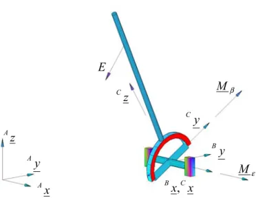
Figure 2.7 shows a massless strut of length L_s joined to the horizontal plane by an universal joint without friction in its moving parts. The support of one of the axis of the universal joint is firmly attached to the ground therefore the joint cannot perform any longitudinal displacement.

The strut is initially in equilibrium and the coordinates of the upper end,

ini

(25)

N F

m L

A S

− − = =

2 0

2 25 . 0

m P ini

A

ú ú ú û ù ê

ê ê ë é

− − =

134 . 0

150 . 0

148 . 0 ,

2

m N M

⋅ =

30 . 0

15 . 0

β ε

Figure 2.7. Data for the static analysis of a strut.

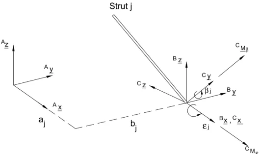
and two constant moments along the axis of the universal joint are applied as it is shown in Figure 2.7. The force AF is expressed in a global reference system whose origin is located at the intersection of the axes of the universal joint. Since the coordinates systems Aand B are coincident, the vector t which represents the location of the origin of the Bsystem with respect to the A system is 0.

It is required to determine the final equilibrium position of the strut and the reaction force and the reaction moment in the support of the strut. The numerical values for P2,ini, AF, and the magnitudes of the moments Mε and Mβare illustrated in Figure 2.7.

z z B

A ,

β M

y

C

y y B

A

,

x x x B C

A , ,

ε

M

z

C

F

A

ini A_P

, 2

s

(26)

Four coordinates systems are defined following the guidelines presented on Figures 2. 3 through 2.5.

System A: global reference coordinate system.

System B: obtained after a translation (0,0,0) of system A. System C: obtained after a rotation _ε about Bx.

System D: obtained after a rotation β about Cy.

Systems A, B and C are shown in Figure 2. 7. With this notation Mε and Mβ expressed in the C system are

m N M

M

C _⋅

ú ú ú û ù

ê ê ê ë é−

=

ú ú ú û ù

ê ê ê ë é−

=

0 0 1 15 . 0 0

0 1 ε

ε (2.45)

m N M

M

C _⋅

=

0 1 0 30 . 0 0

1 0 β

β (2.46)

The strut has 2 degrees of freedom given by the rotations of the universal joint. The solution of the problem consists on finding the value of that rotations, ie

ε and β.

The final position of the upper end of the strut can be found with the aid of (2.36) noting that r=AP2,fin, l=L_s, a=0and b=0.

ú ú ú û ù ê

ê ê ë é

− = =

β ε

β

cos cos

cos sin

sin ,

2

s s

s A

L L

L fin

P

(27)

where r has been expressed in rectangular coordinates instead of homogeneous coordinates. The virtual displacement δr is obtained from (2.2) noting that r=r(ε,β).

δβ β δε ε δ ∂ ∂ + ∂ ∂

= r r

r From (2.47) δβ β ε β ε β δε β ε β ε δ ú ú ú û ù ê ê ê ë é − + ú ú ú û ù ê ê ê ë é − − = sin cos sin sin cos cos sin cos cos 0 s s s s s L L L L L

r (2.48)

Noting that the external force has no ycomponent, the virtual work δW_F

performed by the external force Fis given by

ï þ ï ý ü ï î ï í ì ú ú ú û ù ê ê ê ë é − + ú ú ú û ù ê ê ê ë é − − ⋅ ú ú ú û ù ê ê ê ë é = = δβ β ε β ε β δε β ε β ε δ δ sin cos sin sin cos cos sin cos cos 0 0 . s s s s s F L L L L L Fz Fx r F W

And after simplifying

βδβ ε

βδε ε

βδβ

δW_F =F_xL_Scos −F_zL_Ssin cos −F_zL_Scos sin (2.49) The virtual work due to the external moments δW_M is given by

β δ ε

δ ε

δWM =M ⋅ + Mβ⋅ (2.50)

As the scalar or dot product is invariant under coordinate transformation the last expression can be evaluated easily if the terms on the right side are expressed in the Csystem. Since

(28)

=

0 0 1

ε ε

C _and

=

0 1 0

β β

C

then

δε ε

δ

=

0 0 1

C _(2.51)

and

δβ β

δ

=

0 1 0

C _(2.52)

Substituting (2.45), (2.46), (2.51) and (2.52) into (2.50) the virtual work due to the external moments is simply

δβ δε

δWM = Mε +Mβ (2.53)

The total virtual work is given by the sum of (2.49) and (2.53) and in the equilibrium must be zero, then

0 sin

cos cos

sin

cosβδβ−F L ε βδε−F L ε βδβ+Mεδε+Mβδβ =

L

F_x _S _z _S _z _S

And re-grouping

(

−FzLSsinεcosβ+Mε

) (

δε+ FxLScosβ −FzLScosεsinβ+Mβ

)

δβ =0 (2.54) Since equation (2.54) is valid for all values of δε and δβ which are not in general equal to zero then

(29)

0 cos

sin + =

−FzLS ε β Mε (2.55)

and

0 sin

cos

cosβ −F L ε β+Mβ =

L

F_x _S _z _S (2.56)

For this example the resultant equations (2.55) and (2.56) are not strongly coupled and it is possible to obtain a solution in closed form, however in the most general problems this is not the case and it will be shown that numerical solutions are easier to implement.

A very well known numerical technique is the Newton-Raphson method. The function fsolve of Matlab is used to implement the Newton-Raphson algorithm. In order to use it is necessary to specify the set of equations to be solved, for instance (2.55) and (2.56) in the current example, together with the initial values of and .

The initial values of and , (ε₀ and β₀) can be calculated from (2.37) and (2.38) noting that a=b=0.

134 . 0

150 . 0

tan = − =

z y

o

ε ∴ ε_o =48.2°

÷ ø ö ç

è æ

° − = ÷ ø ö ç è æ − =

2 . 48 sin

15 . 0

148 . 0 sin

tan

ε β

y x

o ∴ βo =−36.3°

With these initial conditions the results given by the software are

o 5 . 72

=

ε and _β ₌₋₇₁_.₇o _(2.57)

(30)

m fin

P

A

ú ú ú û ù ê

ê ê ë é

− − − =

024 . 0

080 . 0

237 . 0 ,

2 (2.58)

The result is illustrated in Figure 2.8.

Figure 2.8. Final equilibrium position of the strut.

A solution by numerical methods is highly sensitive to a correct selection of the initial values. For this example the location of AP2,ini was given explicitly

and this fact permitted to evaluate ε₀ and β₀, but in the analysis of tensegrity structures it is necessary to find them using another approach. This topic will be discussed in detail in Section 3.4.

Table 2.1 shows the results obtained when arbitrarily another set of angles ε₀ and β₀ are chosen as initial guesses. Although the Newton-Raphson algorithm still yields numerical results and that results are equilibrium positions, the solutions listed in Table 2.1 are not compatible with the initial conditions of this exercise. In general if the initial values are not correct the algorithm will not converge to a solution or to find answers that cannot be realized practically.

z

A

y

C

y

A

x

A

z

C

ε β

(31)

Table 2.1. Numerical solutions for different initial conditions. 0

ε β0

35º -20º 18.7º 20.7º

125º 30º 107.5º 71.7º

135º 15º 161.3º -20.7º

Another important consideration to assure the quality of the numerical solutions is to avoid large increments in the input values. It is always possible to increase gradually the value of the external moments and forces, for the static case. In this way the numerical solution is guided without difficulty.

Once the equilibrium position is solved the next step is to evaluate the reaction force and the reaction moment. For this example there is only a single external force and it is applied at the upper end of the strut, and due to the fact systems A and B are coincident, the vector t is zero, as shown in Figure 2.7. For the final equilibrium position of the strut, (2.44) becomes

0 0 0 0 0 0 0 0 0 0 , 2 = ú ú ú ú ú ú ú ú û ù ê ê ê ê ê ê ê ê ë é + ú ú ú ú ú ú ú ú û ù ê ê ê ê ê ê ê ê ë é + ú ú ú ú ú ú ú ú û ù ê ê ê ê ê ê ê ê ë é + ú ú ú ú ú ú ú ú û ù ê ê ê ê ê ê ê ê ë é × z A y A x A z A y A x A z A y A x A A fin A A RM RM RM R R R M M M F P F (2.59) fin A

P2, in (2.59) is given by (2.47). Using this result the first term of (2.59) can be expanded as

(32)

(

)

(

)

(

)

úú

ú ú ú ú ú ú û ù ê ê ê ê ê ê ê ê ë é + − + − = ú ú û ù ê ê ë é × β β ε β β ε ε ε β sin cos sin sin cos cos sin cos cos , 2 y A x A z A x A z A y A z A y A x A A fin A A F F Ls F F Ls F F Ls F F F F P F (2.60)

The external moment is generated by the external moments Mε and Mβ. However they were expressed in the C system, (see Figure 2.7). However (2.59) requires them to be expressed in system A. It is not difficult to establish the geometric relationships between systems C and A. Here the use of the general relations (2.26) to (2.28) is preferred because they are more useful in more complex situations.

As M A

$ is the resultant of Mε and Mβ both expressed in the A system )

$ $

(

$ e C β

C M

A

e +

= (2.61)

where

e: matrix that transforms a line expressed in the C system into the A system. ε

$ C

: Plücker coordinates of CMεin the C system. β

$

C _{: Plücker coordinates of}

β M

C _{in the}_C_system.

Matrix e is obtained using (2.27) and for this case ú û ù ê ë é = R R A R e _A C A C A C 3 3 0 (2.62)

Since the origins of systems A and Care coincident then A₃ (see (2.28)) is given by

(33)

ú ú ú û ù

ê ê ê ë é

=

0 0 0

0 0 0 3

A (2.63)

The rotation matrix AR

C is obtained from the following transformation

ε ,

x B C A B A

CR = R R (2.64)

From Figure 2.7 is apparent that systems A and Bare parallel, then

ú ú ú û ù ê

ê ê ë é

=

1 0 0

0 1 0

0 0 1

R

A

B (2.65)

From Figures 2.4 and 2.7 is clear that system B is obtained after a rotation ε about Bx_{, then}

ú ú ú û ù

ê ê ê ë é

− =

ε ε

cos sin

0

sin cos

0

0 0

1

R

B

C (2.66)

From (2.65) and (2.66) is apparent that

ú ú ú û ù ê

ê ê ë é

− =

ε ε

cos sin

0

sin cos

0

0 0

1

R

A

C (2.67)

(34)

ú ú ú ú ú ú ú ú û ù ê ê ê ê ê ê ê ê ë é − − = ε ε ε ε ε ε ε ε cos sin 0 sin cos 0 0 0 0 1 cos sin 0 0 sin cos 0 0 0 1

e (2.68)

The Plücker coordinates of CMε given by (2.45) are

ú ú ú ú ú ú ú ú û ù ê ê ê ê ê ê ê ê ë é − = 0 0 1 0 0 0

$ε M_ε

C _(2.69)

The Plücker coordinates of CMβ given by (2.46) are

ú ú ú ú ú ú ú ú û ù ê ê ê ê ê ê ê ê ë é = 0 1 0 0 0 0

$β M_β

C _(2.70)

Substituting (2.68), (2.69) and (2.70) into (2.61) yields

ú ú ú ú ú ú ú ú û ù ê ê ê ê ê ê ê ê ë é − = ú ú ú ú ú ú ú ú û ù ê ê ê ê ê ê ê ê ë é = ε ε β β ε sin cos 0 0 0 0 0 0 $ M M M M M M z A y A x A M

A _(2.71)

(35)

x A x

A_R ₌ ₋ _F

y A y

A_R ₌ ₋ _F

z A z

A_R ₌ ₋ _F

(

ε ε

)

ε

β F F M

L

RM A _z

y A S

x

A ₌ _cos _cos ₊ _sin ₊ _(2.72)

(

F cosεcosβ F sinβ

)

Mβcosε

L

RM A _z

x A S x

A ₌ ₋ ₋ ₋

(

F sinεcosβ F sinβ

)

Mβsinε

L

RM A _y

x A S y

A ₌ ₋ ₊ ₋

Recalling the data provided by Figure 2.7 and the results obtained in (2.57) N F A ú ú ú û ù ê ê ê ë é − − = 2 0 2 m L_S =0.25

m N M m N M ⋅ = ⋅ = 30 . 0 15 . 0 β ε ° − = ° = 7 . 71 5 . 72 β ε

The reaction force and reaction moment can be obtained from (2.72). Their numerical values are

m N RM m N RM m N RM N R N R N R z A y A x A z A y A x A ⋅ − = ⋅ = ⋅ = = = = 136 . 0 432 . 0 0 2 0 2

(36)

2.6 Verification of the Numerical Results

As it will be shown in the next chapter the analysis of tensegrity structures involves very complex and lengthy equations. If there is an error in the derivation of the equation the numerical methods still give an answer. However the answer does not of course correspond to the real situation.

It is desirable to verify the validity of the answers obtained using the virtual work approach. Newton’s Third Law assists the verification. Basically the idea is to state the equilibrium equation in such a way that some of the reactions vanish. The resultant equation depends only on the input data and on the generalized coordinates. If the numerical values of the generalized coordinates obtained using the virtual work approach are correct, they must satisfy the equilibrium equations obtained using the Newtonian approach. These concepts are demonstrated using the last example.

The equilibrium equation (2.43) in the C system for the strut of Section 2.5 is

0 $ $ $

$ + + + RM =

C R C M C F C

(2.74)

F C

$ is obtained expressing F A

$ in the C system using (2.29) and (2.30) and noting that the term corresponding to the translation displacement is zero

F A F

C_$ ₌_e−1 _$ _(2.75)

where

ú û ù ê

ë é

=

−

T A C T A C

R O

O R e

3

(37)

R

A

C was obtained in (2.67). Substituting the transpose of (2.67) into (2.76)

yields ú ú ú ú ú ú ú ú û ù ê ê ê ê ê ê ê ê ë é − − = − ε ε ε ε ε ε ε ε cos sin 0 sin cos 0 0 0 0 1 cos sin 0 0 sin cos 0 0 0 1 1

e (2.77)

F A

$ is given by (2.60). Substituting (2.77) and (2.60) into (2.75) yields

(

)

(

)

(

)

úú

ú ú ú ú ú ú û ù ê ê ê ê ê ê ê ê ë é + − + + − + − + = ε ε β β ε β ε β ε ε β ε ε ε ε sin cos sin sin cos sin sin cos sin cos cos cos sin sin cos $ z A y A S z A y A x A S z A y A S z A y A z A y A x A F C F F L F F F L F F L F F F F F (2.78) M C

$ is given by the Plücker coordinates of Mε and Mβ, equations (2.69) and (2.70) ú ú ú ú ú ú ú ú û ù ê ê ê ê ê ê ê ê ë é − = ú ú ú ú ú ú ú ú û ù ê ê ê ê ê ê ê ê ë é + ú ú ú ú ú ú ú ú û ù ê ê ê ê ê ê ê ê ë é − = 0 0 0 0 0 0 0 0 0 0 0 0 0 0 $ β ε β ε M M M M M C (2.79) R C

$ is given by the Plücker coordinates of a force passing through the origin of the C system, therefore it always has the form

(38)

ú ú ú ú ú ú ú ú û ù ê ê ê ê ê ê ê ê ë é = 0 0 0 $ Rz Ry Rx C C C R C (2.80)

Finally in the system C the universal joint cannot provide moment reactions along its moving axes, then C$RM has the form

ú ú ú ú ú ú ú ú û ù ê ê ê ê ê ê ê ê ë é = RMz C RM C 0 0 0 0 0

$ (2.81)

Substituting (2.78), (2.79), (2.80) and (2.81) into (2.74) yields

(

)

(

)

(

)

0 0 0 0 0 0 0 0 0 0 0 0 0 sin cos sin sin cos sin sin cos sin cos cos cos sin sin cos = ú ú ú ú ú ú ú ú û ù ê ê ê ê ê ê ê ê ë é + ú ú ú ú ú ú ú ú û ù ê ê ê ê ê ê ê ê ë é + ú ú ú ú ú ú ú ú û ù ê ê ê ê ê ê ê ê ë é − + ú ú ú ú ú ú ú ú û ù ê ê ê ê ê ê ê ê ë é + − + + − + − + z C z C y C x C z A y A S z A y A x A S z A y A S z A y A z A y A x A RM R R R M M F F L F F F L F F L F F F F F β ε ε ε β β ε β ε β ε ε β ε ε ε ε (2.82) From the forth and fifth rows in (2.82) is possible to define g₁ and g₂ as

(

ε ε

)

ε

β F F M

L

g A _z

y A

S + −

−

= cos cos sin

1 (2.83)

(

F β F ε β F ε β

)

Mβ

L

g A _z

y A x

A

S + − +

= cos sin sin cos sin

(39)

Equations (2.83) and (2.84) involve only the input data and the generalized coordinates and whose values are known from the virtual work approach. After substituting and and the input data into (2.83) and (2.84), g₁

and g₂ must be zero if the values of and correspond to an equilibrium position.

Substituting back the values for L_S, A_F_x_, y A_F _,

z

A_F _{, and given by}

Figure 2. 7 and (2.57) into the last expressions yields 0

15 . 0 ) 5 . 72 sin( ) 2 )( 7 . 71 cos( 25 . 0

1=− − o − o − =

g

0 30 . 0 )) 7 . 71 sin( ) 5 . 72 cos( ) 2 ( ) 7 . 71 cos( 2 ( 25 . 0

2 = − − o − − o − o + =

g

As both g₁ and g₂ vanish, the results obtained using the virtual work for calculating and correspond to an equilibrium position.

(40)

34 CHAPTER 3

GENERAL EQUATIONS FOR THE STATICS OF TENSEGRITY STRUCTURES When an external wrench is applied to a tensegrity structure the ties are deformed and the struts go to a new equilibrium position. This new position would be perfectly defined using the coordinates of the lower and upper ends of the struts in a global reference system. However they are unknown. Equations are developed in this section using the principle of virtual work to solve this problem.

Tensegrity structures exhibit a pattern in their configuration and it is possible to take advantage of that situation to generate general equations for the static analysis. Before starting to implement the method it is necessary to establish the nomenclature for the system and some assumptions to simplify the problem.

Figure 3.1a shows a tensegrity structure conformed by nstruts each one of length L_S. Figure 3.1b shows the same structure but with only some of its struts. The selection of the first strut is arbitrary but once it is chosen it should not be changed. The bottom ends of the strut are labeled consecutively as

n

j E

E E

E₁, ₂, L , , L , where 1 identifies the first strut and n stands for the last strut. Similarly the top ends of the struts are labeled as A₁, A₂, L ,A_j, L ,A_n, as shown in Figure 3.1 b.

(41)

Connecting tie

Top tie

Bottom tie Strut n

Strut 1 Ls

Strut 2

(a)

A

E E

En E

A An Tj

B

A E

Bn L

B

L Ln T

Tn j

j+1

j j j

j+1 1

1

1 1 2

2

(b)

Figure 3.1. Nomenclature for tensegrity structures. a) Generic names; b) Specific nomenclature.

(42)

In every structure it is possible to identify the top ties, the bottom ties and the lateral or connecting ties, as shown in Figure 3.1a. The current length of the top, bottom and lateral ties are called T, B and L respectively.

The top tie T_j extends between the top ends Aj and Aj+1 if j<n and between An and A1 if j=n.

The bottom tie B_j extends between the bottom ends Ej and Ej+1 if j<n and between En and E1 if j=n.

The lateral tie L_j extends between the top end Aj and the bottom

endEj+1 if j<n and between An and E1 if j=n.

In Section 2.3 it was established that the motion of an arbitrary strut can be described by modeling its lower end with a universal joint constrained to move in the horizontal plane. The same model is used now for the derivation of the equilibrium equations for a general tensegrity structure. In addition the following assumptions are made without loss of generality:

• The external moments are applied along the axes of the universal joints.

• The struts are massless.

• All the struts have the same length.

• Only one external force is applied per strut.

• There are no dissipative forces acting on the system.

• All the ties are in tension at the equilibrium position; i.e., the current lengths of the ties are longer than their respective free lengths.

• The free lengths of the top ties are equal.

(43)

• The free lengths of the connecting ties are equal.

• There are no interferences between struts.

• The stiffness of all the top ties is the same.

• The stiffness of all the bottom ties is the same.

• The stiffness of all the connecting ties is the same.

• The bottom ends of the strut remain in the horizontal plane for all the positions of the structure.

3.1 Generalized Coordinates

Due to the fact the lower end of each strut is constrained to move in the horizontal plane and there is no motion along the longitudinal axis since it is constrained by a universal joint, each strut has four degrees of freedom and the total system has 4∗n degrees of freedom which means there are 4∗n

generalized coordinates.

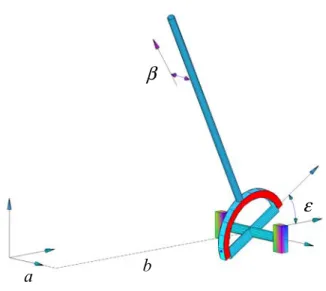
For each strut the generalized coordinates are the horizontal displacements a_j, b_j, as illustrated in Figure 3.2, of the lower end of the strut together with two rotations about the axes of the universal joint. The angular coordinates associated with the strut j are _ε_j and _β_j where _ε_j corresponds to the rotation of the strut about the current Bx axis and β_j corresponds to the rotation about Cy axis, as it was shown in Figures 2.4 and 2.5. Table 3.1 shows the generalized coordinates associated with each strut.

(44)

A

E _z

x y

a b j

j j j

O_A A

A A

Figure 3.2. Coordinates of the ends of a strut in the global reference system A with reference point O_A.

Table 3.1. Generalized coordinates associated with each strut.

Strut Generalized coordinates

1 a₁ b₁ ε₁ β₁

2 a₂

2

b

ε2 β2

M M M M

j _a_j

j

b

ε

_j βj

M M M M M

n a_n

_b

_n

ε

_n β_n

3.2 The Principle of Virtual Work for Tensegrity Structures

Equations (2.10) and (2.11) of Section 2.1 established the conditions for the equilibrium of a system of rigid bodies. The notation used there assumes that the generalized coordinates are grouped in a vector q such that

(

q q qp

)

q = ₁, ₂, .... , where p is the number of generalized coordinates. However, since the notation used for the tensegrity structures differs from Section 2.1, there is only one external force per strut and the moments act only

(45)

along the axes of the universal joint it is more convenient to state the equilibrium equations using the current notation and taking in account the simplifications introduced here.

From (2.3)

c

nc W

W

W δ δ

δ = + (3.1)

where δW is the total virtual work, δW_nc is the virtual work performed for non-conservative forces and moments and δW_c is the virtual work performed by conservative forces. δW_nc can be represented as

M F

nc W W

W δ δ

δ = + (3.2)

where δW_F is the total virtual work performed by non-conservative forces and

M

W

δ is the total virtual work performed by non-conservative moments.

In (2.6) was established that the virtual work performed by the conservative force j, δW_cj is δW_cj = −δV_j where δV_j is the potential energy associated with the conservative force j, therefore the total contribution of the conservatives forces δW_c is

V

W_c δ

δ = − (3.3)

where δV is the summation over all the δV_j present in the structure. Substituting (3.2) and (3.3) into (3.1) yields

V W

W

W δ _F δ _M δ

(46)

In equilibrium the virtual work described by (3.4) must be zero, then the equilibrium conditions can be deduced from

0

= −

+ W V

W_F δ _M δ

δ (3.5)

In what follows each term in the expression (3.5) will be determined. 3.3 Coordinates of the Ends of the Struts

The coordinates of the lower ends can be expressed directly in the global reference system A. The linear displacements associated with the strut j are

j

a and b_j, they correspond to the coordinates x, y measured in the AxAyAz

system. Therefore the coordinates of the lower end Ej expressed in the global

reference system A, (see Figure 3.2), are simply

=

0

j j j

A

b a

E (3.6)

A

E _z

x y

a b j

j j j

O_A A

A A

Figure 3.2. Coordinates of the ends of a strut in the global reference systemAwith reference point O_A.

The coordinates of the upper end of the strut are evaluated with the aid of equation (2.36),

(47)

ú ú ú ú û ù ê ê ê ê ë é + − + = ú ú ú ú û ù ê ê ê ê ë é = 1 cos cos cos sin sin 1 2 β ε β ε β l b l a l z y x P

A _(2.36)

When the angles and for the j-th strut are replaced by ε_jand β_j respectively and l is replaced by L_S, (2.36) yields

ú ú ú û ù ê ê ê ë é + − + = j j s j j j s j j s j A L b L a L A β ε β ε β cos cos cos sin sin (3.7)

Now it is possible to obtain expressions for the lengths of the top, bottom and lateral ties.

The lengths of the top ties T are given by

(

)

(

)

(

)

(

₂

)

1/2

1 2 2 1 2 2 1 2

1 Ax Ax A y Ay A z Az

T = − + − + −

(

)

(

)

(

)

(

₂

)

1/2

2 3 2 2 3 2 2 3

2 Ax A x A y A y Az A z

T = − + − + −

M

(

) (

)

(

₂

)

1/2

, , 1 2 , , 1 2 , ,

1x jx j y jy j z jz j

j A A A A A A

T = ₊ − + ₊ − + ₊ − (3.8)

if j =n then j+1=1

The lengths of the bottom ties B are given by

(

)

(

)

(

)

(

₂

)

1/2

1 2 2 1 2 2 1 2

1 E x Ex E y E y E z Ez

B = − + − + −

(

)

(

)

(

)

(

₂

)

1/2

2 3 2 2 3 2 2 3

2 E x E x E y E y E z E z

B = − + − + −

M

(

) (

)

(

₂

)

1/2

, , 1 2 , , 1 2 , ,

1x jx j y jy j z jz j

j E E E E E E

(48)

if j =n then j+1=1

The lengths of the lateral ties L are given by

(

)

(

)

(

)

(

₂

)

1/2

2 1 2 2 1 2 2 1

1 Ax E x Ay E y Az E z

L = − + − + −

(

)

(

)

(

)

(

₂

)

1/2

3 2 2 3 2 2 3 2

2 A x E x A y E y Az E z

L = − + − + −

M

(

) (

)

(

₂

)

1/2

, 1 ,

2 , 1 ,

2 , 1

,x j x jy j y jz j z j

j A E A E A E

L = − ₊ + − ₊ + − ₊ (3.10)

if j =n then j+1=1

3.4 Initial Conditions

In the example of Section 2.5 it was established that the numerical methods are highly sensitive to the selection of the initial values. The problem of the initial position of a tensegrity structure, this is the position of the structure in its unloaded position were addressed by Yin [1]. In this section his results are presented without proof and are adapted to the current nomenclature.

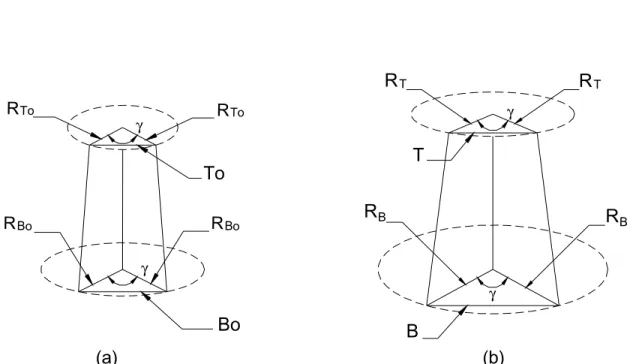
The free lengths of the top and bottom ties and the current lengths of the top and bottom ties satisfy the relations illustrated in Figure 3.3, therefore

2 sin 2

0 o_γ

T

R = (3.11)

2 sin 2

0 o_γ

B

R = (3.12)

2 sin

2R_T γ

T = (3.13)

2 sin

2R_B γ

(49)

where T₀ and B₀ are the free lengths of the top and bottom ties respectively and T and B are the current lengths of the top and bottom ties for the unloaded position. The angle γ depends on the number of struts and is given by

n

π

γ = 2 (3.15)

where n is the number of struts

Bo To

R

T

B

γ

γ γ

γ

T To

Bo RTo

Bo R

R T

R

RB R_B

(a) (b)

Figure 3.3. Relations for the top and bottom ties of a tensegrity structure. a) Ties with their free lengths; b) Ties after elongation.

In the unloaded position the quantities R_T, R_B and the current length of the lateral ties L satisfy the following equations

(

)

0

2 sin 2

1 ÷ − − =

ø ö ç

è

æ ₋ γ

To T

T B

o

L R k R R

L L

k (3.16)

(

)

0

2 sin 2

1 ÷ − − =

ø ö ç

è

æ ₋ γ

Bo B

B T

o

L R k R R

L L

(50)

(

)

[

cos cos

]

0

2

2 ₊ ₊ ₋ ₌

− Ls RBRT α γ α

L (3.18)

where

T

k : stiffness of the top ties.

B

k : stiffness of the bottom ties.

L

k : stiffness of the lateral ties.

S

L : length of the struts. 0

L : free length of the lateral ties.

α : angle related to the rotation of the polygon conformed by the top end with respect to the polygon conformed by the bottom ends of the struts and is given by

n

π π

α = −

2 (3.19)

The solution of (3.16), (3.17) and (3.18) can be carried out numerically. Once R_B, R_T (and L) have been evaluated the values of T and B are calculated from (3.13) and (3.14).

Summarizing, when the free lengths of the top, bottom and lateral ties of a tensegrity structure are given, together with their stiffness, strut lengths and number of struts, equations (3.16), (3.17) and (3.18) yield the current values of the top, bottom and lateral ties in its unloaded position.

Although in the work of Yin [1], the following relations are not established explicitly, it can be shown that if the global reference system A is oriented in such a way that its x axis passes through the bottom of one of the struts when the structure is in its unloaded position, then the coordinates of the top and lower

(51)

ends of the strut for its initial position in a global reference system A, (see Figure 3.4), are