MODELLING OF STOCK PRICES BY THE MARKOV CHAIN MONTE CARLO METHOD

MODELLING OF STOCK PRICES BY THE MARKOV CHAIN

MONTE CARLO METHOD

Mantas LANDAUSKAS

Kaunas University of Technology, Faculty of Fundamental Sciences Studentų 50, LT - 51368 Kaunas, Lithuania

mantas.landauskas@ktu.lt Eimutis VALAKEVIČIUS

Kaunas University of Technology, Faculty of Fundamental Sciences Studentų 50, LT - 51368 Kaunas, Lithuania

eimval@ktu.lt

Abstract. Th is paper presents a universal approach to modelling stock prices. Th e tech-nique involves Markov Chain Monte Carlo (MCMC) sampling from piecewise-uniform distri-bution.

Today’s fi nancial models are based on assumptions which make them inadequate in many cases. One of the most important issues is determining the distribution of a stock price, its re-turn or other fi nancial mean. Th e approach proposed in this paper removes almost all presump-tions from a distribution of a stock price. Th e probability density must be evaluated using some nonparametric estimates. Th e kernel density estimate (KDE) suits well for that purpose. It gives a smooth and presentable estimate.

MCMC was chosen due to its versatility and is applied to KDE using piecewise-linear dis-tribution as proposal density. Th e proposal density is constructed according to the KDE. Such link between the piecewise-linear distribution’s simplicity and relative massiveness of KDE bal-ances together.

Involving the kernel density estimate and the methodology to sample from it makes the technique universal for modelling any real stochastic system while having empirical data only and barely any assumptions about the distribution of it.

JEL classifi cation: C10, C15, C46, C65.

Keywords: Stock prices, Markov chain, Monte Carlo method, MCMC, kernel density, piecewise-linear distribution.

Reikšminiai žodžiai: Akcijų kainos, Markovo grandinė, Monte Karlo metodas, branduoli-nis tankis, dalimis tolygusis skirstinys.

INTELLECTUAL ECONOMICS 2011, Vol. 5, No. 2(10), p. 244–256

Classical model of stock prices has some assumptions about fi nancial data. It can-not be applied to model the stock price having returns which are can-not log normally distributed.

Th ere are several approaches to model diffi cult quantities, but they specialize in diff erent areas. Th e purpose of this paper is to present a universal technique for model-ling stock prices. Th is technique consists of special numerical methods and is suitable for any empirical data.

Th e Markov chain Monte Carlo method is used to sample from empirical prob-ability density of a stock price. Th e technique is fl exible and requires just the ability to calculate probability at any given point. Furthermore, MCMC was successfully applied to one-factor models for the interest rate (B. Eraker, 2001). Th is also acts as the reason-ing for choosreason-ing it for this approach of modellreason-ing stock prices.

It is also needed to approximately evaluate empirical probability density. Th is is performed using kernel density estimation. Th e link between these two methods is considered and this leads to apply it on every fi nancial data.

1. Monte Carlo Modelling of Stock Prices

Th e process of a stock price is treated as a Brownian motion. Th us its value satisfi es the equation:

(1.1) Consider a fi nancial mean with log normally distributed returns. Th e random walk of price of such a fi nancial mean is modeled according this formula (P. Wilmott, 2007):

(

t t

) ( )

S t e t tZ

S

Δ + Δ ⎟ ⎠ ⎞ ⎜ ⎝ ⎛ −

= Δ

+ δ σ σ

2 2 1

. (1.2) Here random value Z~N

( )

0,1 follows standard normal distribution, δ is annual risk free return and σ is annual standard deviation of the logarithm of a stock price.

2. Markov chain Monte Carlo (MCMC)

Suppose it is needed to generatexi ~π

( )

x . When xi ~π

( )

x is diffi cult to sample from, MCMC sampling technique could be performed. In fact MCMC is a set of techni-ques used for this purpose. Th e main idea of it is to construct a Markov chain

{ }

Xi ∞i₌0,

such that

(

X x

) ( )

x P i

i→∞ = =π

A Markov chain is predefi ned by an initial state P

(

X0 =x0

) ( )

=g x0 and the

tran-sition kernel P

( ) (

y x =P X_i+1= y X_i =x

)

. Stationary distribution

( )

( )

i i f x x

∞ →

=lim π

is unique if the chain is ergodic. Th en:

( )

_∑

( )

( )

Ω ∈ = x x y P x y π

π , ∀y∈Ω. (2.2)

Latter equality could be rewritten as a set of (n−1) linear equations:

( ) ( )

(

)

( )

(

)

( )

(

)

( ) ( )

(

)

( )

(

)

( )

(

)

⎪ ⎩ ⎪ ⎨ ⎧ + + + = + + + = ; ... ... ; ... 2 2 1 1 2 2 2 2 1 2 1 2 n n n n n n n n x x P x x x P x x x P x x x x P x x x P x x x P x x π π π π π π π π (2.3)

here n:= Ω. Th ere are a total number of (n−1) equations and n

( )

n−1 transition prob-abilities P

( )

xj xk , k =1,n, j=1,n−1. Th us there exist an infi nite number of transi-tion kernels P

( )

y x , such that the stationary distribution of the Markov chain is π

( )

x .

One of the techniques used for constructing such a transition kernel is Metropolis-Hastings algorithm (J.S. Dagpunar, 2007). Th e idea of it is to choose any other transi-tion kernel Q

( )

y x . Th en there exists a probability that Q

( )

y x is equal to P

( )

y x .

(2.4) Considering the detailed balance condition of a time-homogeneous Markov chain yields:

(2.5) Th e general solution for (2.5) is . It is necessary to have a higher acceptance ratio when sampling random numbers, therefore by adjust-ing r

( )

x,y and considering higher acceptance ratio while sampling random numbers (V. Prokaj, 2009) it is shown that:

( )

( )

_{( )}

( )

_{( )}

_⎟⎟ ⎠ ⎞ ⎜ ⎜ ⎝ ⎛ = x y Q x y x Q y x y π π

α min 1, . (2.6)

3. Nonparametric probability density estimation

Consider a sample consisting of random independent and identically distributed values Xi. Kernel density estimate is chosen for evaluate the probability density of Xi.

( )

_∑

(

)

= − = n i i h x X K n x f 1 1

ˆ _,

( )

_⎟

⎠ ⎞ ⎜ ⎝ ⎛ = h x K h x Kh 1 , (3.1) here K

()

⋅ is the kernel function, h is its width.

(3.2)

Below are some kernel functions that are frequently used. Th e triangular kernel function is useful if the data has sharp edged distribution. Gaussian kernel makes the estimate’s PDF plot very smooth.

( )

⎩ ⎨ ⎧

> ≤ −

=

. 1 ,

0

, 1 ,

1

x x x x

K _{(triangular), (3.3)}

(Yapanichnikov), (3.4)

( )

2

2

2

1 x

e x

K = −

π (Gauss). (3.5)

Basically, such probability density estimation is about assigning kernel density to each Xi and including weighted sum of all other assignations. Th e contribution of any other X _j to the probability value at X_i is smaller if X_i − X_j is bigger.

Fig. 1. Kernel density estimation.

Figure 1 shows the probability density estimation from 5 given points while ap-plying Gaussian kernel. Th e estimate is absolutely smooth. Th e only drawback of such

estimation is the necessity of using all the points from the sample while evaluating the probability at a particular point.

4. A New Approach to Modelling Stock Prices 4.1. Evaluation of Distribution Function

Th is chapter presents the approach to model stock prices or any other statistical data (the method is universal enough) without knowing analytical probability density function.

First of all kernel density estimation must be performed and construct an estimate to the return of a stock price. At this point there could be a discussion if this estimate is accurate, but it is assumed to be exact. And there is no need to look for analytical func-tions which best fi t in a particular case. It is not necessary to think about the shape at all, it forms itself according the data. Th e only question is the width of the kernel function.

4.2. Special technique for constructing a proposal density

Th e target probability density is now constructed. In order to model it a special technique is required, because there are no inverse cumulative density function or one cannot represent the estimate using known analytical PDF’s. MCMC is a solution but it could not be applied directly to the PDF estimate mentioned before.

Probably the biggest advantage of MCMC is the ability to generate required density using the proposal density, which should be similar in shape to target density. No other requirements to proposal density. Th us the complexity of proposal density is as simple as it is needed. Consider a histogram, which is relatively fast and simple non-paramet-ric estimate for target density. It is possible to use it as proposal density therefore. But the assumption about target density not being discrete must be taken in mind, there are no set of values to construct a histogram from. Th e idea of the technique presented in this paper is to construct a piecewise-uniform distribution according to the kernel density estimate. A piecewise-uniform distribution is defi ned in eq. (4.2.1).

(4.2.1)

Th e area below the probability density function must be equal to 1, thus:

0 1

1 x x q

n n

i i

− =

∑

−

. (4.2.2) Th is distribution is treated as a proposal density. Generating random numbers from this distribution is fast and simple.

Fig. 3. Generating random numbers using inverse CDF.

Sampling from q

( )

x requires application of a search procedure. Firstly a u~U

( )

0;1 is drawn. Th en it is required to fi nd the interval

(

xi,xi−1

]

, i=1,n, to which u belongs

to. Since the number of intervals is going to be small, this step does not require many calculation steps. Th en u is mapped to x according to the CDF of q

( )

x like in fi gure 3. CDF of q

( )

x is obtained by calculating the area below target density in each of the intervals.

Using q

( )

x as the proposal density and kernel density estimate as a target distribu-tion implies random values xi having distribution equal to fˆ

( )

x . It must be noted that

acceptance ratio for xi is now

( )

( ) ( )

_{( ) ( )}

_⎟⎟ ⎠ ⎞ ⎜

⎜ ⎝ ⎛ =

y q x f

x q y f x

y

ˆ ˆ , 1 min

Th e sampling technique is called the independence Metropolis-Hastings when

( )

x y q

( )

x

q = . Th e independence sampler has one signifi cant advantage compared to traditional Metropolis-Hastings: the sequence

{ }

xi has no memory eff ect. Each ran-dom value accepted in simulation process does not depend on previous value. Th us there is no importance in what was x0 generated. A brief description of

Metropolis-Hastings techniques could be found in (M. Johannes, 2006).

5. Calibration of the model

Every model should give adequate results and compare to other known models or techniques. Making the model hold this is called a calibration. In this case, the new technique for modelling stock prices must give similar results as traditional Monte Carlo if stock returns are log normally distributed. Again the hypotheses about the normality of the logarithms of the stock returns are going to be tested.

Fig. 4. Yahoo! Inc. historical share prices.

Yahoo! Inc. (YHOO) share prices from 2010 01 04 to 2010 09 27 were chosen for performing the calibration. Historical share prices are depicted in fi gure 4. By perform-ing the Kolmogorov-Smirnov test on the logarithms of the prices’ returns p=0.992 and D=0.0742 were obtained. D< p shows that the logarithms are normally dis-tributed and leads data to be suitable for classical stock price model.

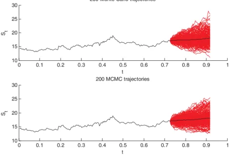
Fig. 5. Classical Monte Carlo modelling versus MCMC approach.

200 trajectories (fi gure 5) were modeled for each technique. According the classi-cal Monte Carlo approach the mean value of a price aft er 50 days will be 18.08 $. Th e newly proposed technique gave it 18.10 $ per share. Th is is actually expected, because the trend was considered.

Fig. 6. Comparing Monte Carlo and MCMC results.

In fi gure 6 the histograms of classical Monte Carlo and MCMC are compared. Th ey represent the distribution of stock prices at the end of the modelling process. Th e modelling process contained 1000 paths of a stock price and simulated 100 days. Th us it required 100000 random stock returns to be performed.

Fig. 7. Diff erences between the Monte Carlo and MCMC results.

Th e biggest diff erence between the two histograms exists at about mean value. Th e tails match better. Classical Monte Carlo converges to stock price distribution when the number of paths is increasing; the method proposed in this paper should also. Checking if the new method matches Monte Carlo is equivalent to checking if it converges to the distribution of a stock price. While evaluating the diff erence between two probability densities oft en an integral of an absolute value of their diff erence is used. Now consider an estimate:

(5.1)

and is the histograms of a stock price at the end of the modelling, m is number of bars and X_j represents the center point of the j -th bar.

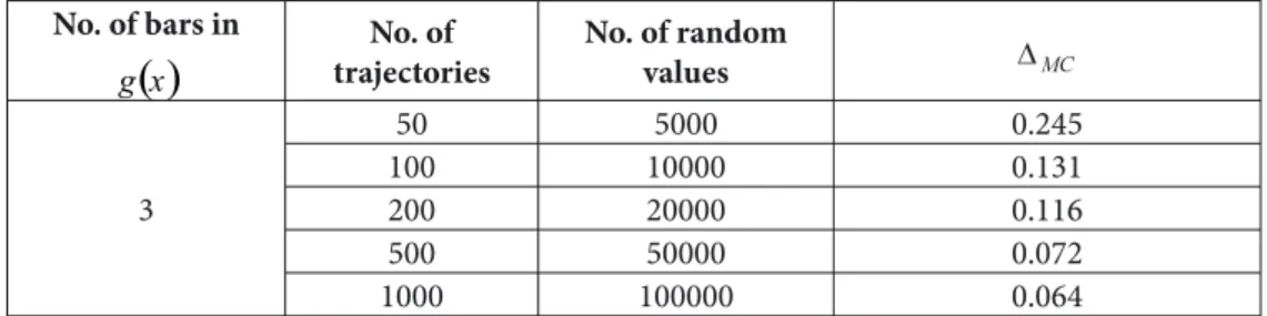
Table 1. Diff erences between the histograms of the stock prices modeled by Monte Carlo and MCMC

No. of bars in

( )

x g

No. of trajectories

No. of random values

3

50 5000 0.245

100 10000 0.131

200 20000 0.116

500 50000 0.072

1000 100000 0.064

Table 1 shows how changes if the number of a stock price paths N increases. Th e bigger N the more Monte Carlo and MCMC results are alike. MCMC proved to be suitable for modelling stock prices.

Th e number of bars in g

( )

x is equal to a question of peaks and distance between them in target distribution. Since the returns of stock prices have a distribution similar

( )

to best match the target distribution.

Table 2. Diff erences between the histograms of the stock prices modeled by Monte Carlo and MCMC

No. of bars in g

( )

x No. of trajectories

No. of random values

5

50 5000 0.265

100 10000 0.131

200 20000 0.091

500 50000 0.060

1000 100000 0.050

As the table 2 shows choosing 5 bars in proposal density results in more precise distribution of stock prices. Accuracy increases but the calculation time is higher also. Th is is due to more calculation steps required to fi nd the interval of g

( )

x to which a particular random number belongs to.

6. Modelling stock prices

Here is an example when classical Monte Carlo method cannot be applied to mod-el stock prices.

Fig. 8. Distribution of normalized logarithms of continuous day returns.

Th e histogram of normalized logarithms of continuous day returns Ri of Tesco

Corporation (TESO) is depicted in fi gure 8. Although the hypothesis of normality is ac-cepted, there exist two peaks. If one is confi dent about the shape of histogram, the as-sumption of normality should be rejected and standard Monte Carlo cannot be applied.

Fig. 9. Forecasting the stock prices.

Constructing kernel density estimate for

1 1

− −

− =

i i i i

S S S

r using Gaussian kernel

function also gives PDF with 2 peaks (fi gure 9). MCMC with piecewise-linear distribu-tion as a proposal density was applied to this PDF.

Fig. 10. Forecasting TSO stock prices.

Average share price aft er 50 days resulted in $14.75. All the prices generated are distributed according kernel density estimate. Sampling is based entirely on empirical data and has no assumptions about PDF.

7. Conclusions

1. While estimating the probability density of a custom stock return with kernel density, each return in the sample is considered.

2. Proposed technique for modelling stock prices leads for average path of the stock price having small dispersion. Th e same holds for the Monte Carlo method.

ability density leads to better accuracy of distribution modeled, but requires more time to perform the method.

4. Combining MCMC with kernel density estimate leads the technique for being able to model any real system. Th us empirical probability density is construct-ed using particular statistical information. Th is could be value of a fi nancial mean, product quality measures and so on. Th us the technique is universal.

References

1. B. Eraker. MCMC Analysis of diff usion models with applications to fi nance. Journal of Business and Economic Statistics, vol. 19, pp. 177-191, 2001.

2. J. S. Dagpunar. Simulation and Monte Carlo. John Willey & Sons Ltd., Great Britain, Chippenham, Willtshire, 2007.

3. M. Johannes, N. Polson. MCMC Methods for Continuous-Time Financial Econometrics, 2006. <http://www0.gsb.columbia.edu/faculty/mjohannes/PDFpapers/JP_2006.pdf>. 4. P. Wilmott. IntroducesQuantitative Finance, 2ed. JohnWilley& Sons Ltd., 2007.

5. V. Prokaj. Proposal selection for mcmc simulation. Applied Stochastic Models and Data Analysis, pp. 61–65, 2009.

AKCIJŲ KAINŲ MODELIAVIMAS MARKOVO GRANDINĖS MONTEKARLO METODU

Mantas Landauskas Eimutis Valakevičius

Santrauka. Straipsnyje pristatoma universali akcijų kainų modeliavimo technika. Ši tech-nika paremta Markovo grandinių Monte Karlo (MCMC) metodo taikymu modeliuojant dali-mis tolygųjį skirstinį.

Dabartiniai fi nansų rinkų modeliai paremti prielaidomis, kurios dažnai juos verčia neadek-vačiais. Viena didžiausių problemų yra akcijos kainos, jos grąžos ar bet kokios kitos fi nansinės priemonės pasiskirstymo dėsnio nustatymas. Šiame straipsnyje pasiūlytas požiūris pašalina praktiškai visas prielaidas apie akcijos kainos pasiskirstymą. Tokiu atveju pasiskirstymo dės-nis turi būti įvertintas neparametriniu būdu. Branduolidės-nis tikimybinio tankio įvertinimas šiam tikslui puikiai tinka. Jis sudaro glotnų ir reprezentatyvų tankio įvertį.

MCMC buvo pasirinktas dėl didelio pritaikomumo ir yra taikomas branduoliniam tan-kio įverčiui su dalimis tolygiuoju skirstiniu kaip alternatyviu (aproksimuojančiu) tankiu. Alternatyvus tankis konstruojamas pagal branduolinį įvertį. Toks dalimis tolygiojo skirstinio paprastumo ir santykinai aukšto branduolinio tankio įverčio sudėtingumo skaičiavimo prasme apjungimas sukuria balansą tarp šių metodų.

Naudojant branduolinį akcijos kainos pasiskirstymo įvertinimą ir šiame straipsnyje siū-lomą jo modeliavimą padaro pateiktą techniką universalią. Ji tampa tinkama bet kokiai realiai stochastinei sistemai turint tik jos empirinius duomenis ir beveik jokių prielaidų apie jų pasis-kirstymą.

Mantas Landauskas is a postgraduate student in applied mathematics at Faculty of Fundamental Sciences, Kaunas University of Technology. Master’s degree research area: model-ling of stochastic systems by MCMC method.

Mantas Landauskas - Kauno technologijos universiteto Fundamentaliųjų mokslų fakulteto taikomosios matematikos magistrantas. Magistro darbo tyrimų tematika: stochastinių sistemų modeliavimas taikant MCMC metodą.

Eimutis Valakevičius – Doctor, Associated professor. Faculty of Fundamental Sciences, Kaunas University of Technology. Diploma Applied mathematics, VU (1978), PhD (1989), Associated Professor (1991), Head of Department of Mathematical Research in Systems (1997-2001). Author of more than 70 publications (monograph, textbooks, research results, study guides and projects). Research interests: modeling of stochastic systems, numerical modeling of fi nancial markets.

Eimutis Valakevičius – Kauno technologijos universiteto Fundamentaliųjų mokslų fakulteto Matematinės sistemotyros katedros docentas, daktaras. 1978 m. baigė VU taikomosios matematikos specialybę, 1989 m. įgijo daktaro laipsnį, 1997-2001 m. vadovavo matematinės sis-temotyros katedrai. Paskelbė virš 75 publikacijų. Mokslinių interesų sritis – stochastinių sistemų bei fi nansų rinkų modeliavimas.