Degree-Driven Design of Geometric Algorithms for
Point Location, Proximity, and Volume Calculation
David L. Millman
A dissertation submitted to the faculty of the University of North Carolina at Chapel Hill in par-tial fulfillment of the requirements for the degree of Doctor of Philosophy in the Department of Computer Science.
Chapel Hill 2012
Approved by:
Jack Snoeyink
David P. Griesheimer
Ming C. Lin
Dinesh Manocha
c
2012
Abstract
DAVID L. MILLMAN: Degree-Driven Design of Geometric Algorithms for Point Location, Proximity, and Volume Calculation
(Under the direction of Jack Snoeyink)
Correct implementation of published geometric algorithms is surprisingly difficult. Geomet-ric algorithms are often designed for Real-RAM, a computational model that provides arbitrary precision arithmetic operations at unit cost. Actual commodity hardware provides only finite pre-cision and may result in arithmetic errors. While the errors may seem small, if ignored, they may cause incorrect branching, which may cause an implementation to reach an undefined state, produce erroneous output, or crash. In 1999 Liotta, Preparata and Tamassia proposed that in ad-dition to considering the resources of time and space, an algorithm designer should also consider the arithmetic precision necessary to guarantee a correct implementation. They called this design techniquedegree-driven algorithm design. Designers who consider the time, space, and precision for a problem up-front arrive at new solutions, gain further insight, and find simpler representa-tions. In this thesis, I show that degree-driven design supports the development of new and robust geometric algorithms.
I demonstrate this claim via several new algorithms. For n point sites on a U × U grid I consider three problems. First, I show how to compute the nearest neighbor transform in O(U2) expected time,O(U2)space, and double precision. Second, I show how to create a data structure in O(nlogU n) expected time,O(n)expected space, and triple precision that supports O(logn)
Acknowledgments
I thank my fiancée Dr. Brittany Terese Fasy for her never ending love and support. Whether down the street or on the other side of the world, her encouragement could be heard all over. Thank you Brit!
I thank my adviser Dr. Jack Snoeyink for all that he has taught me while at UNC. Thank you for always pushing me to think more abstractly, write more clearly, and present more engagingly. I also thank my other committee members: Dr. David P. Griesheimer, Dr. Ming Lin, Dr. Dinesh Manocha, and Dr. Chee K. Yap for their suggestions, discussions, and time committed to serving on my committee.
The work in the dissertation work would not have been possible without the support of De-partment of Energy, Bettis Atomic Power Laboratory, National Science Foundation, Google, Lime Connect, and UNC-Chapel Hill. Two years of this research were performed under appointment of the Rickover Fellowship program in Nuclear Engineering sponsored by the Naval reactor division of the US Department of Energy. I thank all involved with the fellowship program and the technical and administrative support staff of UNC.
I thank my co-authors: Dr. Vicente H. F. Batista, Dr. Timothy Chan, Steven Love Dr. Brian Nease, Matt O’Meara, Dr. Sylvain Pion, Dr. Johannes Singler, and Clarence R. Willis. In par-ticular, I thank co-author Vishal Verma for participating in our productive (and sometimes not so productive) research discussions.
Cochran, Srinivas Krishnan, Alana Libonati, and Catie Welsh for making me remember that the world isn’t just grid points and bisectors. There is no better way to end the week than with a trip to Bandido’s or a walk to get coffee. I thank Doug McNamara for cheering so loudly for me.
Table of Contents
Abstract . . . iii
List of Figures . . . xii
List of Tables . . . xiv
1 Introduction . . . 1
1.1 Thesis Statement and Contributions . . . 3
2 Background . . . 6
2.1 Floating Point Representation . . . 6
2.2 Definitions of Correctness . . . 7
2.3 Previous Results in Degree-Driven Algorithm Design . . . 12
3 Analyzing the Precision of Predicates, Constructions and Algorithms . . . 16
4 Degrees of Predicates and Constructions . . . 24
4.1 Constructions . . . 25
4.1.1 Line(a, b) . . . 27
4.1.2 Plane(a, b, c) . . . 28
4.1.3 Bisector(a, b) . . . 30
4.1.5 VoronoiVertex(a, b, c) . . . 32
4.2 Predicates and Simple Algorithms . . . 33
4.2.1 PointOrdering(a, b) . . . 33
4.2.2 Orientation(a, b, q) . . . 34
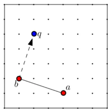
4.2.3 Closer(a, b, q) . . . 35
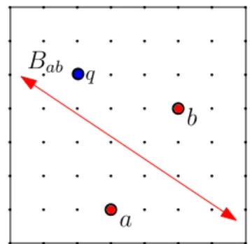
4.2.4 SideOfABisector(Bab, q) . . . 36
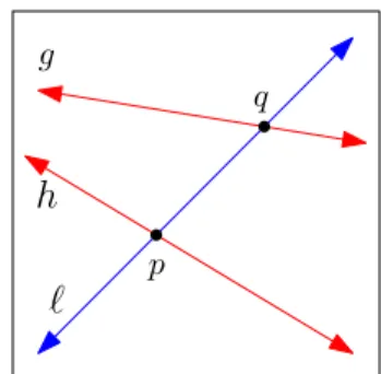
4.2.5 OrderOnLine(Bab, Bcd, `) . . . 36
4.2.6 OrderOnLine(g, h, `) . . . 37
4.2.7 InCircle(a, b, c, q). . . 37
4.2.8 IntersectInterior(ac, bd) . . . 38
4.3 Checking Preconditions . . . 39
4.3.1 Equal Homogeneous Coordinates . . . 40
4.3.2 Preconditions for Points . . . 40
4.3.3 Preconditions for Lines . . . 41
5 Irreducibility of Polynomials . . . 42
5.1 Notation . . . 42
5.2 Basket Weaving Technique for Proving Irreducibility . . . 43
5.3 Polynomials from Determinants of Matrices with Independent Variables . . . 44
5.4 PointOrdering(a, b)is Irreducible . . . 46
5.5 VoronoiVertex(a, b, c)Cannot be Simplified . . . 47
5.6 Orientation(a, b, q)is Irreducible . . . 48
5.7 SideOfABisector(Bab, q)andCloser(a, b, q)are Irreducible . . . 51
5.8 OrderOnLine(Bab, Bcd, `)is Irreducible . . . 52
5.9 OrderOnLine(l, h, `)is Irreducible . . . 53
6 Gabriel Graph . . . 56
6.1 Introduction . . . 56
6.2 Arrangements of Dual Lines . . . 57
6.3 Algorithm Description . . . 58
6.4 Conclusion . . . 62
7 Point Location . . . 63
7.1 Introduction . . . 63
7.2 Definitions and Notation . . . 65
7.2.1 The Voronoi Diagram and Grids . . . 65
7.2.2 Trapezoidation and Point Location . . . 68
7.3 Computing Point Location Structures with Triple Precision . . . 70
7.3.1 The Reduced-Precision Voronoi Diagram . . . 71
7.3.2 Constructing the Reduced-Precision Voronoi Diagram . . . 72
7.4 Computing Point Location Structures with Double Precision . . . 79
7.4.1 Definitions and Notation . . . 80
7.4.2 Constructing the D2-Voronoi Diagram . . . 84
7.5 Conclusion . . . 90
8 Nearest Neighbor Transform . . . 91
8.1 Preliminaries . . . 92
8.1.1 Previous work . . . 92
8.1.2 Definitions . . . 93
8.1.3 Problem transformations . . . 94
8.1.4 Geometric primitives . . . 95
8.2.1 Discrete Upper Envelope . . . 97
8.2.2 NNTrans Algorithm . . . 102
8.3 Experiments . . . 104
8.4 Conclusions . . . 108
9 Volume Calculation . . . 109
9.1 Model Representation . . . 113
9.1.1 Primitives: Signed Quadric Surfaces . . . 113
9.1.2 Component Hierarchy: Boolean Formulae . . . 114
9.1.3 Problem Statement . . . 116
9.2 Divide and Conquer Using Predicates . . . 117
9.2.1 Surface/Axis-Aligned Box Classification . . . 117
9.2.2 Component/Box Classification and Restriction . . . 123
9.3 Volume Estimators . . . 124
9.3.1 Error bounds . . . 126
9.4 Experiments . . . 127
9.5 Conclusions . . . 130
10 Using Degree-driven Algorithm Design to Achieve EGC . . . 132
10.1 EGC Technique 1: Static Analysis . . . 133
10.2 EGC Technique 2: Software Implementations . . . 133
10.3 EGC Technique 3: Arithmetic Filters . . . 134
10.4 EGC Technique 4: Adaptive Evaluation . . . 135
10.5 Conclusion . . . 137
A Sign of a Sum . . . 138
List of Figures
3.1 Intersection coordinate not lending itself to a floating point representation. . . 16
4.1 Line(a, b)produces the line thoughaandb. . . 27
4.2 Plane(a, b, c)produces the plane thougha,b, andc. . . 28
4.3 Bisector(a, b)produces the perpendicular bisectorab. . . 30
4.4 LineIntersection(`, h)produces the intersection point of`andh. . . 31
4.5 VoronoiVertex(a, b, c)produces the point equidistant toa,b, andc. . . 32
4.6 The pointaprecedes the pointb. . . 33
4.7 The path fromatobtoqforms a right turn. . . 34
4.8 The query pointqis on the same side of theBab asb. . . 36
4.9 The bisectorBab is above the bisectorBcdon the line`. . . 36
4.10 The intersection ofg and`is left of the intersection ofhand`. . . 37
4.11 The query pointqin inside the circumcircle ofa,bandc. . . 37
4.12 The segmentsacandbdintersect. . . 38
6.1 Gabriel graph of sites. . . 57
6.2 If sitesj kills(s, si)from the left, it also kills all edges right ofsiand left ofsj. . . 59
7.1 Trapezoidation of a small Voronoi diagram and a piece of the trapezoid graph. . . . 68
7.2 Voronoi vertices in a grid cell contracting to two rp-vertices. . . 72
7.3 Constructing the rp-Voronoi diagram. . . 73
7.5 The four cases per wall for bisector tracing. . . 75
7.4 A bisector entering a grid cell from the south. . . 75
7.7 Voronoi polygons, proxy trapezoidation, and Voronoi trapezoidation. . . 81
7.8 Illustration ofGCDWalk. . . 85
7.9 New sitesiin conflict with Voronoi trapezoidτ. . . 87
8.1 Transforming sites inS to linesLY(S). . . 95
8.2 Adding a set of lines to a DUE. . . 98
8.3 Constructing and updating the possible lists. . . 102
8.4 The three steps of the NNTrans algorithm. . . 103
8.5 Time-per-pixel box plots of 100 runs ofUsqon varying densities and grid sizes. . . 106
8.6 Time-per-pixel for four implementations varying grid sizes and densities. . . 107
8.7 Time-per-pixel for four implementations on images from the MPEG7 data set. . . . 108
9.1 HierarchyNp-N-Nc, with comp.C(N)striped purple and blue. . . 115
9.2 Intersection of a quadric with an axis-aligned plane. . . 117
List of Tables
4.1 Summary of primitive types. . . 26 4.2 Summary of constructions. . . 26 4.3 Summary of predicates. . . 27
Chapter 1
Introduction
The representation of numbers makes a difference in the ease of doing correct calculation. InThe Elements, Euclid spoke of numbers as geometric measures and observed that the √2, and other numbers, could not be represented as a fractions of integer measures—that it was irrational. With computers we face the opposite question: how to represent geometry with numbers. Rather than using geometry to represent a number, we may, for example, want to calculate the intersection point of two lines and store the coordinates in memory. We then need to know how many bits of memory are sufficient to store the point accurately. Computers have brought new questions about designing and analyzing algorithms for solving problems that can be stated geometrically; these algorithms we callgeometric algorithms.
are practical, researchers seek to minimize the asymptotic growth of processor time and memory space as the problem sizes grow, and (with some famous exceptions) tacitly agree not to use the power afforded by unbounded precision in each cell. Inprecision analysisthe number of bits used to represent numbers is analyzed and minimized as well. In this thesis I investigate designing geometric algorithms by considering all three: time, space, and precision.
My main study is predicates, which are tests that control branching in geometric algorithms. Segregating numerical computation on input coordinates into predicates not only enables preci-sion analysis, but also increases the chances that an algorithm will be correctly implemented, since predicates can be separately tested, debugged, and put into libraries for reuse. In this thesis, I restrict my attention topredicatesthat test signs of polynomials in the input coordinates, and con-structions that produce objects defined by rational polynomials in the input coordinates. Liotta, Preparata, and Tamassia suggested that we can bound the precision required by a geometric algo-rithm by analyzing the degree of predicates. Thus, thedegree of my algorithms is the degree of their highest degree predicate.
In most efficient geometric algorithms it is common for predicates to take many times the precision of the input coordinates. To evaluate a degree 5 predicate on 32-bit input coordinates would require approximately 160 bits (about five times the number of bits for representing the input coordinates). As most machines only support 64-bit arithmetic, unless higher precision is simulated in software, for some inputs the test will be wrong.
1.1
Thesis Statement and Contributions
In this thesis, I show that degree-driven analysis supports the development of new and robust geometric algorithms. The contributions are summarized in the remainder of this section.
One of the early developments in computational geometry was the identification of predicates for various geometric tests. The design and implementation of algorithms were based on a lim-ited set of predicates, rather than on numerical coordinates. Thus, we consider representations of primitives (such as points and lines) and predicates on these primitives. Chapter 3 describes how precision will be analyzed in this thesis and Chapter 4 derives and upper bounds the precision of many common predicates.
The easiest way to reduce the precision of a predicate is to factor its polynomial. It is often claimed that the polynomials in common predicates cannot be factored but is rarely shown and references are rarely provided. Chapter 5 shows that the polynomials from Chapter 4 cannot be factored and identifies some helpful techniques for showing that a polynomial cannot be factored.
The next four chapters support the thesis statement by using degree-driven analysis to give new and robust algorithms for the Gabriel graph, post-office queries, nearest neighbor transform and volume calculation of CSG models. Let me briefly define these problems and state the main results.
Gabriel Graph. First, given a setS withnpoint sites, an edge(si, sj)withsi, sj ∈ S is in the Gabriel graph ofSif the edge maintains the Gabriel property, that is, the closed disk with diameter
sisj contains no points ofS besidessi andsj. Testing if an edge has the Gabriel property can be
Post-Office Queries. Second, given a query pointq and a setS withnpoint sites, a post-office
queryreturns the site ofS closest toq. Forsi, sj ∈ S, testing ifqis closer tosi orsj is degree 2. Thus, there is a simple brute force linear time degree 2 algorithm for queries, test q against all sites. More efficient algorithms preprocess the point set to achieve O(logn) time queries. The standard algorithm [31] computes the Voronoi diagram of S, which takes O(nlogn) time and degree at least 4; computes the trapezoid map of the Voronoi edges, which takes timeO(nlogn)
and degree 5; and queries the map, which naively takesO(logn)time and degree 6 (however, it is easy to reduce such queries to degree 3). Chapter 7 presents areduced precision Voronoi diagram that forn sites on aU ×U grid, can be computed inO(nlogU n)expected time,O(n)expected space, and degree 3. The reduced precision Voronoi diagram supportsO(logn)time and degree 2 post-office queries. The chapter concludes with the description of a degree 2 Voronoi diagram that can be constructed with degree 2 and supportsO(logn)degree 2 post-office queries.
Chapter 2
Background
A computer supports a subset of the reals called floating point numbers. In Section 2.1, I de-scribe the IEEE standard for representing floating point numbers. Since a computer cannot repre-sent all reals, designers (and implementers) of geometric algorithms may have different definitions of what it means for an algorithm to be correct (or have a correct implementation). In Section 2.2, I describe the two main paradigms to correctness, Topology-Oriented Computation [127] and Exact Geometric Computation [140]. One way to achieve the goals of exact geometric computation is to reduce the amount of precision required by an algorithm. Liotta, Preparata, and Tamassia [89] sug-gested a guideline called, degree-driven algorithm design for upper bounding the precision required by an algorithm. In Section 2.3, I survey the previous work in degree-driven algorithm design.
2.1
Floating Point Representation
In the IEEE 754 standard for binary floating point format a number is represented as a sign s, exponent e, and mantissa m1. The sign is 1 bit, and the exponent and mantissa are some fixed number of bits (dependent on representation and precision). In anormalizedfloating point repre-sentation, the highest order bit of the mantissa is assumed to be 1 and so it does not need to be
1The base is sometimes called the radix, the mantissa is sometimes called thesignificandand the exponent is
explicitly represented. Often a biasis added to the exponent to simplify comparisons. The value of a normalized floating point number with biasEis(−1)s×1.m×2e−E.
This familiar representation was not always so common. In a 1998 interview[120], Kahan recalls some of the peculiarities of early implementations of floating point arithmetic. For example, two floating point values could test as not-equal, yet their difference could be zero. Kahan, along with Coonen and Stone proposed the IEEE Standard 754-1985, which is the basis for the “float” and “double” types in many high level programming languages such as C, C++, C#, and Java. In these languages, “float” is implemented by the IEEE 754-2008 single precision floating point format calledbinary32 (in IEEE 754-1985 it was calledsingle) with 1 bit for the sign, 8 bits for the exponent and 23 bits for the mantissa. In fact, binary32 specifies a floating point number as
(−1)s×(1 + Σ23
i=1bi2−i)×2e−127.
The set ofbinary32numbers is finite, so only a subset ofRcan be represented exactly. The rest of the numbers must be approximated. For example, even a simple rational such as1/3must be rounded to a number near0.3. For arithmetic operations, the result of a floating point operation on floating point input is the same as the result of the true operation on the floating point input rounded to one unit in the last place. IEEE standard allows for multiple rounding modes. Of particular importance are “round up” and “round down”, which round toward positive and negative infinity respectively. The two rounding modes are the basis for arithmetic filters, which are discussed further in Chapter 10.
2.2
Definitions of Correctness
predicates to be evaluated incorrectly and cause implementations to fail [44, 63].
One could naively rely on machine precision and replace comparisons against zero with com-parisons against an-tolerance. Kettneret al.[75] investigate the errors introduced with floating point arithmetic using simple predicates, such asOrientation, and generate simple examples where an incremental convex hull algorithm fails. Their numerical experiments show that the errors of a floating point based orientation predicate have a complex and non-intuitive structure. Kettner also points out that-tolerances do not fix the problems raised by their investigation; by rounding non-zero values to zero, it only enlarges the complex error structure.
Instead, one could add steps to ensure correct results. Yap [141] calls the study of algorithms with running time dependent on the precision of the input or output, numerical computational geometry. Below I outline what I believe to be the two main paradigms of numerical computational
geometry,Topology-Oriented ComputationandExact Geometric Computation.
Topology-Oriented Computation (TOC). Geometric algorithms often aim to compute struc-tures for which topological properties may hold even if the geometry is perturbed. For example, the Voronoi diagram is a connected planar graph, that happens to have convex faces in its geometric embedding. Suighara [127, 128, 131] proposes that algorithms be designed to guarantee chosen topological properties (e.g., connectedness or planarity), even if the geometric embedding con-tains perturbations or numerical error (e.g., self-intersections or non-convexities). His Topology-Oriented Computation paradigm seeks to ensure that, at a minimum, geometric algorithms should fail gracefully as they reach the limit of the available precision.
Suighara defines TOC more formally [128], let P be a geometric problem in whichX is the set of inputs toP andY is the set of outputs. Letf be an algorithm for solvingP andfebe an implementation off. Iffeis implemented with finite precision arithmetic, for x ∈ X the output
e
of the implementationfe.
For a concrete example, letP be the problem of computing the Voronoi diagram of sites with double precision floating point coordinates in 2D. An inputx isn distinct sites with double pre-cision floating point coordinates. The output is the Voronoi diagram of the n sites. Let f be Fortune’s algorithm [43] andfebe Brubeck’s [17] implementation of Fortune’s algorithm. For an inputx ∈ X, fC(x) is a planar graph, andfN(x)the coordinates of the graph’s vertices and the directions of the infinite edges. Brubeck reports that his implementation does not terminate for all input. But for all xfor which fe(x)terminates, fCe (x)and fNe (x)are the graph and the vertex coordinates reported byfe, respectively.
Suighara [128] defines the implementationfeto berobustiffeis defined for anyx∈X. That is, for anyx∈ X,fe(x)does not crash or go into an infinite loop. Note that the outputfe(x)may not be inY. The implementationfeistopologically consistentif for allx∈X,fCe (x)∈fC(X). Note that this does not mean that fCe (x) = fC(x)or even thatfCe (x) is in the neighborhood offC(x); simply that there is some inputy∈X such thatf(y) = fe(x).
Sugihara with others proposed robust and topologically-consistent algorithms for many prob-lems including, solid modeling with planes [129], divide-and-conquer construction of Voronoi diagrams of points in 2D and 3D[107, 65, 66], incremental construction of the Voronoi dia-grams of polygons [64], and gift-wrapping and divide-and-conquer constructions of convex hull in 3D [126, 102, 103]. TOC can create robust implementations. Sugihara and Iri [130] used TOC to create an algorithm for building the first Voronoi diagram of over a million sites with single precision arithmetic. (It should be noted that Isenburg et al. [67] used EGC, described in the next section, to build the first Voronoi diagram of over a billion sites with single precision input.) Held and Huber [56] used TOC to create the first floating point implementation for computing the Voronoi diagram of circular arcs (without discretizing or approximating the arcs).
in no way similar to the correct output. Consider the following topologically consistent algorithm for computing the Voronoi diagram. As a preprocess, select a point setx, and by hand compute the Voronoi vertices and edges forx. At run time, for any inputyreturn the Voronoi vertices and edges forx. Moreover, few of the classic geometric algorithms designed using the Real-RAM model are robust, let alone topologically consistent. Thus, many of the classical geometric algorithms are not correct under the definitions of TOC.
Exact Geometric Computation (EGC).Geometric computing is part combinatorial, for
ex-ample traversing an embedded graph, and part numeric, for exex-ample determining if two segments intersect. Yap [140] observes that the interplay between the numerical and the combinatorial is what causes geometric algorithms to be difficult to implement. His Exact Geometric Computation paradigm dictates that an algorithm’s control flow should be independent of the machine on which the implementation is run; in particular, it should be the same as if the algorithm was implemented with real arithmetic.
The strength of EGC is that it cleanly separates the algorithm design process from the number types used in an implementation. By abstracting the number type away from the programmer, de-bugging and implementation become easier. Indeed, EGC’s strength can be seen in its acceptance in software development. Well-known open-source software libraries CGAL [2] and LEDA [19] both have geometric kernels that support EGC.
The weakness of EGC is pointed out originally by Yap [140] and revisited by Held and Mann [57]. The easiest way to implement EGC is to use software to simulate rational or real arithmetic. When done blindly, simulating with software can be slow. Karasicket al.report that directly using ratio-nal arithmetic caused a10,000xslowdown [72]. However, with the knowledge that the important computation is the signs of polynomials and a bit of work, the slowdown can be reduced to below
10x. In Chapter 10, I outline the major techniques used for implementing EGC.
approximate coordinates are needed. Without care, the approximate results may introduce fatal errors. For example, consider computing the convex hull of a set of segment intersection points and outputting its polygonal boundary as a list of vertex coordinates. The rounded coordinates may cause the boundary of the convex hull to be non-convex. Geometric rounding [32, 49, 51, 55, 58, 60] investigates how to round a construction’s coordinates while maintaining the important geometric and topological properties.
Perhaps more seriously is that if number types are abstracted too early in the design process, an algorithm may perform unnecessary constructions. Let’s see an example that takes a bit to explain. Acascading constructionis a phenomenon where constructions are used to create more construc-tions2. A common industrial example of cascading constructions occurs in polyhedral modeling systems. Consider a system (similar to Maya [1]) in which the polyhedra are represented by in-tersecting a set of half-planes. A common operation is to output the boundary of the polyhedra. Often the boundary is represented as: a set of vertices, defined by coordinates; a set of polygonal faces, defined by an ordered list of pointers to vertices; and adjacencies between faces.
It is common to build the boundary incrementally. Assume that we have constructed the bound-ary ofPi−1defined by the firsti−1planes. When adding planepi, find all vertices outside of the constraints implied bypi. Throw away all faces outside ofpi and split all faces intersected by pi. Splitting faces introduces new vertices, update the vertices and the topology of the polyhedra. Of-ten, in implementation, due to numerical errors, the resulting set of vertices defining a polygon are not coplanar as they would be in Real-RAM. Thus, a face may not have a clearly defined normal.
Suighara and Iri [129] observed that the cascading constructions are unnecessary, and are in fact a source of error. They observed that vertices do not need to be represented by coordinates. Instead, they can be represented by triples of planes defining them. Burnstein and Fussell [8] used
2The classic example of a cascading construction is thePentagonproblem, proposed by Dobkin and Silver [35],
this observation and some additional predicate evaluation techniques to build a modeling system that is faster than CGAL [2], which uses exact arithmetic, and is more stable than Maya, which uses floating point arithmetic.
Burnstein and Fussell’s implementation is fast and stable because they avoid high precision tests used by other implementations. In particular, they use low precision predicates to reduce the need for simulating real arithmetic. Thus, when designing an algorithm (or implementing a pre-existing algorithm) it is worth paying attention to how much precision is used.
This thesis explores Liotta, Preparata, and Tamassia’s proposed degree-driven algorithm de-sign[89] guideline. This guideline seeks to optimize (and balance) running time, space, and preci-sion simultaneously. Once we know how much precipreci-sion is required by an algorithm, creating an efficient implementation that follows EGC becomes easier. The EGC implementation techniques described in Chapter 10 are still relevant. But degree-driven algorithm design allows a programmer to make more informed decisions on when the techniques are needed.
2.3
Previous Results in Degree-Driven Algorithm Design
The most complete study of degree-driven design was carried out for segment intersection prob-lems [10, 11, 21, 90]. Boissonnat and Preparata [10] describe three probprob-lems for a set of n line segments defined by their endpoints with single precision coordinates:
P1 report all pairs of intersecting segments;
P2 construct the arrangement of the segments;
P3 construct the trapezoid graph of the segments.
Fornsegments we can have Θ(n2)intersections. A trivial algorithm with worst-case optimal running time is to check all pairs using a double precision segment intersection test. However, more interesting algorithms consider the number of intersectionsk. Boissonnat and Preparata show that a degree 3 variant of the degree 5,O((n+k) logn)time Bentley-Ottmann sweep line algorithm [7] solves P1 inO((n+k) logn)time. They also show that P1 for red and blue segments with only bichromatic intersections can be solved with degree 2.
Chan [21], and Boissonnat and Snoeyink [11], investigate degree-driven algorithm design by using a restricted set of predicates and abstract the above/below test on curve segments (whose degree is dependent on the complexity of the carrier of the curve). Boissonnat and Snoeyink con-sider segment intersection problems on a set of pseudo-segments, which arex-monotone segments such that any pair have at most one point in their intersection. They show that when limited to the three tests: ordering of endpoints; checking if an endpoint, in the vertical slab defined by a segment, is above or below the segment; and testing if two curves intersect; P1 is lower bounded byΩ(n√k). They also show that for segments, Balaban’s [6] degree 3,O(nlogn+k), algorithm can be modified to degree 2 with a slight loss of efficiency, running inO(nlog2n+klogn)
time3. Finally, they show that even with restricted predicates, the red-blue intersection problem (with pseudo-segments) can be solved inO(nlogn+k)time.
As touched upon in almost all the literature on degree-driven algorithms for segment inter-sections, but most clearly stated by Mantler and Snoeyink [90], P2 requires four-fold precision, and P3 requires five-fold precision. Mantler and Snoeyink consider P2 for red and blue segments. They show that the topology of arrangement (but not the coordinates of the intersections) can be computed using a sweep line algorithm that runs in optimalO(nlogn+k)time usingO(n)space and degree 2.
3Boissonnat and Snoeyink’s degree 2 version of Balaban’s algorithm appears to be the first example of a
Researchers also consider point location queries. Given a set of npoint sites where the coor-dinates of the sites and query points are b-bit integers. Let U = 2b, and the set of representable
points from which sites and queries are picked is aU×U grid, sometimes referred to as a universe of sizeU [25].
Liotta, Preparata and Tamassia [89] describe a degree 6 algorithm for rounding a trapezoidation of the Voronoi diagram to a degree 1 data structure capable of reporting nearest neighbor queries inO(logn)time with degree 2. Unfortunately, they still have to construct the trapezoidation. Mill-man and Snoeyink [99] consider how to construct Liotta’s structure with a degree 3 randomized algorithm in a sizeU universe in timeO(nlogU n). We will see this algorithm in Chapter 7. Using a different approach, Millman and Snoeyink [100] describe a degree 2 construction of a degree 1 data structure supporting degree 2 logarithmic time point location queries. We further explore this construction in Chapter 7.
To compute the nearest neighbor for all query points in a universe of sizeU with degree 2, we could simply test all query points against all sites to achieve anO(nU2)algorithm. Millmanet al. [98] show how to compute all nearest neighbor queries using degree 2 predicates with an expected timeO(U2)algorithm, which we encounter in Chapter 8.
The additively weighted Voronoi diagram is a generalization off the Voronoi diagram in which a sitesis defined by a centercand a weightwand the distance between a pointpin the plane and
s iskp−ck −w. Karavelas and Yvinec [73] proposed a degree 14 algorithm for computing the
additively weighted Voronoi diagram. In previous work [96], I showed that the predicates presented by Karavelas and Yvinec could be simplified to degree 6. The new predicates, implemented in CGAL [2], resulted in a 39–66% speed up in predicate evaluation and a 10-20% reduction in the number of calls to software arithmetic for nearly degenerate inputs.
The Gabriel graph of a sizenpoint setSis an embedded graph. The vertices are the points ofS
Chapter 3
Analyzing the Precision of Predicates,
Constructions and Algorithms
c
= (1
,
0)
d
= (1
,
2)
b
= (0
,
3)
q
= (
13,
83)
a
= (0
,
4)
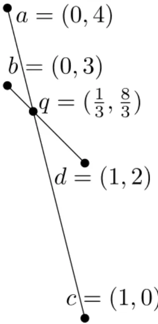
Figure 3.1: Two segments with an intersection coordi-nate that does not lend itself to a floating point representa-tion.
This thesis explores designing geometric algorithms and seeks to optimize the running time, space and precision. Analysis of al-gorithms in terms of time and space is commonly studied in a stan-dard algorithms classes; see [30]. Analyzing the precision of an al-gorithm, however, is not so well known. Thus, the purpose of this chapter is to define terms that are central to the thesis and famil-iarize the reader with guidelines for upper bounding the precision required by an algorithm. I illustrate the important definitions and analysis on the example problem:
DoSegsIntersect Given two, two-dimensional line-segments, ac
We assume that no three points are collinear so that we may avoid unnecessary details that de-tract from the purpose of this chapter. Full details for intersecting segments are given in Chapter 4 where we remove the assumption.
In this thesis, I assume that the inputs to a geometric algorithm are a set of numeric coordinates scaled to b-bit integers and combinatorial relationships between the coordinates. Sometimes, I refer to the precision of the input coordinates asdegree 1orsingle precision. InDoSegsIntersect, the numerical coordinates are thexandyvalues of the segment endpoints, and the combinatorial relationships are the pairing of values into points and the pairing of points into segments.
ForU = 2b, it is sometimes helpful to consider the coordinates as integers in{0, . . . , U−1}. In
such a case, when the input are points are planar, we can imagine them as laying on aU×Uinteger grid which we callU. We assume that the input is scaled to an integer grid because as Chan and Pˇatra¸scu [25] point out, the floating point plane is the union of integer grids with different scalings around the origin. The problems in this thesis are translation independent. Thus, the ability to have more precision for input near the origin is not particularly helpful.
Apredicateis the sign of a multivariate polynomial with variables from the input coordinates. A positive, negative, or zero result can be interpreted geometrically. Often, the interpretation is used in algorithms to make branching decisions. Consider the predicate:
Orientation(a, b, c): Given single precision coordinate values of 2D pointsa,b, andc,
Orientation(a, b, c) = sign(bxcy −bxay −axcy −cxby+cxay +axby). (3.1)
The predicate’s positive, negative, or zero result has the geometric interpretation that the path fromatobtocmakes a left turn, makes a right turn, ora,bandcare collinear, respectively. For the segments shown in Figure 3.1,Orientation(a, c, d)is a left hand turn,Orientation(a, c, b)
Thedegree of a predicateis the degree of the polynomial. Thus,Orientationis degree 2. Degree notation is a helpful bookkeeping device for analyzing the degree of polynomials where we represent a degreek polynomial as
k . When it is clear from the context we may drop thesignfunction. Thus, the predicateOrientation(a, c, b) =
2 .Boissonnat and Preparata [10], define the degree of a predicate as the maximum degree of its ir-reducible factors. Even though I show that most of the predicates used in this thesis are irir-reducible, I omit the irreducibility condition. As we will see in Chapter 5, showing that a multivariate poly-nomial is irreducible is cumbersome (and not necessary for proving upper bounds). I hope that by omitting the irreducibility condition and simplifying precision analysis, degree-driven algorithm design can become of interest to a larger audience.
By removing the irreducibility condition the difference in degree may be substantial. For ex-ample, for variables X = {x1, . . . , xn}, the polynomial formed by expanding the determinant of the Vandermonde matrix
V1(X) =
1 x1 x21 . . . x
n−1 1
1 x2 x22 . . . xn
−1 2 ..
. ... ... . .. ...
1 xn x2
n . . . xnn−1
has polynomial degree n(n −1)/2. The polynomial can be rewritten as a product of linear fac-tors [136],V2(X) =
Q
1≤i<j≤n(xj−xi). This factorization means that the predicate,sign(V2(X)), is degree 1. If we didn’t know of the factorization, however, the predicatesign(V1(X))would be degreen(n−1)/2.
in this thesis, the coefficients of monomials in a predicate are small constants (usually 2 or 4), a monomial of degreekcan be evaluated withbk+O(1)bits. Moreover, in this thesis, the number of variables in a predicate is small, says. Forsvariables, the number of monomials in a polynomial isO(sk)and a polynomial of degreekcan be evaluated withbk+O(1) +klog
2sbits. Thus, the calculation of a predicate can be carried out ink(b+O(1)) bits. The degreek can be thought of as the leading term, determining the required precision. Just as we ignore constants in time and space analysis, we ignore carry bits from addition and coefficients in this analysis. In Chapter 10 we discuss implementation techniques that can sometimes be used to reduce the number of bits.
A construction is an operation that produces a new object from the coordinate values of the input. Consider the construction producing the intersection pointqof lines←ac→and←bd→.
Intersect(a, c, b, d) takes the single precision coordinate values of four two-dimensional points
a,c,b, anddand produces the coordinates of the intersection point of non-parallel lines←ac→
and←bd→. The construction returns the pointq, whose coordinates are:
qx =
axcy−cxay ax−cx
bxdy−dxby bx−dx
ax−cx ay−cy
bx−dx by −dy
, qy =
axcy −cxay ay−cy
bxdy −dxby by −dy
ax−cx ay −cy
bx−dx by−dy
. (3.2)
We can extend degree notation to the operations {+,×}. Let f and g be polynomials with coefficients inR. One can show that
deg(f g) = deg(f) + deg(g) and deg(f) + deg(g)≤max(deg(f),deg(g)).
The equalitydeg(f) + deg(g) = max(deg(f),deg(g))holds when addingf andgdoes not cause all highest degree monomials to cancel. In this thesis, degree notation may only be used with operations when all highest degree monomials do not to cancel. Define the operations{+,×}for
a
, b , c , and d as:a
+ b =max(a, b)a
× b =a+b a b + c d =max(a+d, c+b)
b+d a
b × c d =a+c
b+d .
Next, I present a typical solution forDoSegsIntersectreducing it to a previously solved prob-lem. If precision is a concern then I would not suggest using this solution. It is, however, useful for illustration purposes. In Algorithm 1, SegsIntByConstruction solvesDoSegsIntersectby constructing the intersection pointqof the lines through our segments and testing properties ofq.
The degree of an algorithmis the maximum degree of its predicates and constructions. Let’s see an example of precision analysis carried outSegsIntByConstruction. The algorithm tests if←ac→is parallel to←bd→, in line 1. As each slope is degree 1 over 1, by clearing fractions, we check if the lines are parallel with degree 2. That is, we test if the predicate
Algorithm 1 SegsIntByConstruction(a, c, b, d): Determine if ac and bd intersect; if so return INTERSECT, if not return NOINTERSECT
Require: no three points are collinear
1: if←ac→k←bd→then
2: return NOINTERSECT 3: end if
4: Pointq=Intersect(a, c, b, d) /* See Equation 3.2 */
5: Realt1 = (qx−ax)/(cx−ax)
6: Realt2 = (qx−bx)/(dx−bx)
7: ift1 ∈(0,1)&t2 ∈(0,1)then
8: return INTERSECT 9: else
10: return NOINTERSECT 11: end if
is zero. TheIntersectconstruction, in line 4, computes the Cartesian coordinates ofq, which we saw before are degree 3 over 2. Solving fort1 andt2, in lines 5 and 6 respectively, is degree 3 over 3. That is,
t1 =
qx−ax cx−ax =
3
/2 − 1 1 =3
/2 − 2 /2 1 =(
3 −2 )/21
=3
/21
=3
3
,and similarly fort2. Next, we see thatt1 andt2are in(0,1), in line 7, with degree 3. Lett1 =n/d. Bothnanddare degree 3. We test ift1 ∈(0,1)by checking if:
(sign(n)<0 and sign(d)<0 and sign(n−d)>0) or (sign(n)>0 and sign(d)>0 and sign(n−d)<0).
In an implementation of the typical solution, the coordinates ofq would often be represented in floating point. Floating point values are a subset of R, thus most real values must be rounded (see Section 2.1 for more on floating point representation) For a real value x, let fl(x) be its floating point representation. For a geometric objectodefined by coordinate values,fl(o)is the geometric object induced by applying flto the coordinate values of o. For example, the point
fl(q)has coordinate values(fl(1/3),fl(8/3)). Sometimes the difference betweenqandfl(q)
is negligible. In Figure 3.1, however,fl(q)does not lie on either segment.
Instead, consider an algorithm that avoids the possibly erroneous construction of an intersection point. The algorithm uses the observation thatacintersectsbdif and only ifaandcare on opposite sides ofbdandbanddare on opposite sides ofac.
In Algorithm 2,SegsIntByOrientation, we useOrientationto determine if the two segments intersect by checking if the endpoints ofbdare on opposite sides of←ac→and the endpoints ofacare on opposite sides of←bd→.
Algorithm 2SegsIntByOrientation(a, c, b, d): Determine ifacandbdintersect; if so return INTERSECT, if not return NOINTERSECT
Require: no three points are collinear
1: ifOrientation(a, c, b)6=Orientation(a, c, d)
andOrientation(b, d, a)6=Orientation(b, d, c)then
2: return INTERSECT 3: else
4: return NOINTERSECT 5: end if
TheSegsIntByOrientationalgorithm avoids the construction of an intersection coordi-nate and arrives at a simpler algorithm. It uses the predicate in Equation 3.1, which is degree 2. The four Orientation predicates, in line 1, evaluate only Equation 3.1, so it too is degree 2. Thus,SegsIntByOrientationis degree 2.
Chapter 4
Degrees of Predicates and Constructions
Geometric primitives, such as lines and points, may be represented by numbers in the computer in several ways. For example, a line can be specified as the coordinates of two points, as a slope and intercept, or as three coefficients of a homogeneous equation ax+by+cw = 0. Even for points there are choices of Cartesian, polar, or signed homogeneous coordinates [124, 125].
In this chapter, I define geometric predicates and constructions that are needed by the algo-rithms throughout the thesis. I focus on representations of primitives for which the predicates and constructions evaluate polynomials; in the next chapter, I show that the polynomials for the pred-icates that are defined here are irreducible. This chapter concludes with a discussion of verifying the preconditions for the predicates and construction. The results of both chapters, 4 and 5, are summarized in Tables 4.1 to 4.3.
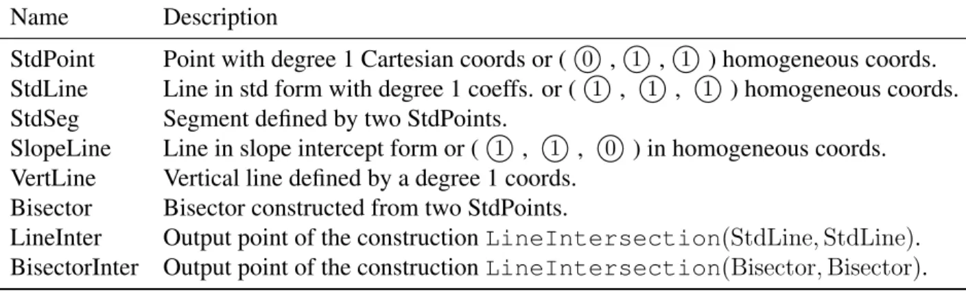
Table 4.1 names representations of points and lines that the algorithms use. Signed homogeneous coordinates [124, 125] unify the representations. In short, a tuple (w, x, y) with w 6= 0
represents the Cartesian point (x/|w|, y/|w|) with a spin that is clockwise if w < 0 and counter-clockwise if w > 0. A tuple with w = 0 represents the point at infinity in the direction(x, y). We call two points (or lines)aandbdistinctif there is noλ∈R\ {0}such
denote a coordinate of degreekas
k .For example, Cartesian point (x, y) has homogeneous representation (1, x, y), which we write as (
0 , 1 , 1 ) because we care primarily about the degrees of the input co-efficients in our analysis. Similarly, an input line specified by the coco-efficients homoge-neous equation(c, a, b)·(w, x, y)T = 0is(1 ,
1 ,
1 ), while an input line specified in
slope/intercept form is(
1 , 1 , 0 ).Table 4.2 summarizes the degrees of constructions of points and lines that are named and derived in the indicated sections of this chapter. For example, the first line in the table tells us that the construction Line(a, b) takes as input two StdPoints a and b and produces a line
1
x+ 1 y+ 2 = 0 or in homogeneous form (2 , 1 , 1 ). The derivation forLineis found in Section 4.1.1.
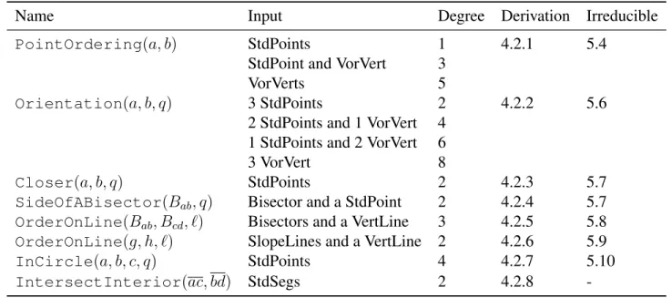
Table 4.3 summarizes the degrees of the predicates on points and lines. For example, the first three rows in the table tells us that PointOrdering(a, b)for two StdPoints is degree 1, for a StdPoint and a Voronoi vertex is degree 3 (regardless of whether the Voronoi vertex is
aorb), and for two Voronoi vertices is degree 5. The derivations are given in Section 4.2.1
and irreducibility is shown in Section 5.4.
4.1
Constructions
A geometric construction produces a new geometric object from the input. Here we consider the degrees of some well-known and useful constructions that appear regularly throughout this thesis1.
1All constructions in this section have at least one precondition, such as the input points need to be distinct. When
Table 4.1: Summary of point and line types that are input to predicates and constructions.
Name Description
StdPoint Point with degree 1 Cartesian coords or (
0 ,1 ,1 ) homogeneous coords. StdLine Line in std form with degree 1 coeffs. or (1 , 1 , 1 ) homogeneous coords. StdSeg Segment defined by two StdPoints.SlopeLine Line in slope intercept form or (
1 , 1 , 0 ) in homogeneous coords. VertLine Vertical line defined by a degree 1 coords.Bisector Bisector constructed from two StdPoints.
LineInter Output point of the constructionLineIntersection(StdLine,StdLine). BisectorInter Output point of the constructionLineIntersection(Bisector,Bisector).
Table 4.2: Summary of constructions of points and lines.
Name Input Output Derivation
Line(a, b) StdPoints Line: (
2 , 1 , 1 ) 4.1.1Plane(a, b, c) StdPoints Plane: (
3 , 2 , 2 , 2 ) 4.1.2Bisector(a, b) StdPoints Line: (
2 , 1 , 1 ) 4.1.3LineIntersection(`, h) StdLines Point: (
2 , 2 , 2 ) 4.1.4 Bisectors Point: (2 , 3 , 3 )SlopeLines Point: (
1 , 1 , 2 )Table 4.3: Summery of predicates.
Name Input Degree Derivation Irreducible
PointOrdering(a, b) StdPoints 1 4.2.1 5.4 StdPoint and VorVert 3
VorVerts 5
Orientation(a, b, q) 3 StdPoints 2 4.2.2 5.6 2 StdPoints and 1 VorVert 4
1 StdPoints and 2 VorVert 6
3 VorVert 8
Closer(a, b, q) StdPoints 2 4.2.3 5.7
SideOfABisector(Bab, q) Bisector and a StdPoint 2 4.2.4 5.7
OrderOnLine(Bab, Bcd, `) Bisectors and a VertLine 3 4.2.5 5.8
OrderOnLine(g, h, `) SlopeLines and a VertLine 2 4.2.6 5.9
InCircle(a, b, c, q) StdPoints 4 4.2.7 5.10
IntersectInterior(ac, bd) StdSegs 2 4.2.8
-A construction is preformed on coordinates of the input. Recall that we assume that input coordinates are degree 1, which areb-bit integers. For a universe of sizeU = 2b, we can think of
the set of all points with degree 1 Cartesian coordinates as lying on aU ×U gridU.
4.1.1
Line
(
a, b
)
a b
`
Figure 4.1: Givena, b∈ Uin
red, construction Line(a, b)
produces the line ` in blue, throughaandb.
Often, the line defined though two distinct pointsa, b∈U, depicted
in Figure 4.1, is {ta+ (1−t)b | ∀t ∈ R}. When ax 6= bx, we represent the line by algebraically expanding the equation y−ay
x−ax =
by−ay
bx−ax, arriving at the standard and slope-intercept forms,
standard form: 0 = (ay−by)x+ (bx−ax)y+ (axby−aybx)
slope-intercept form: y= by −ay
bx−axx+
(aybx−axby)
bx−ax .
standard form is 0 =
1 x + 1 y + 2 and in slope-intercept form is y = 1 /1 x+ 2 /1 . The fraction means that the slope of the line through two points is a rational polynomial of degree 1 over 1 and they-intercept is degree 2 over 1. This line representation, however, does not support orientation.When orientation matters, we use the definition of a line from oriented projective geome-try [125, Chapter 5.1]. For two distinct points a and b, the line from a to b is defined by the joina∨b(see [125, Chapter 5.4] for more on the join). The line froma tobcan be written as a determinant equation:
aw ax ay
bw bx by
w x y
= (axby −aybx)w−(awby−bway)x+ (awbx−bwax)y= 0
For a homogeneous coordinate q = (qw, qx, qy)let¬q = (−qw, qx, qy), that is the spin of the coordinate is reversed. One can derive two useful identities about oriented lines. First thata∨b=
¬(b∨a), which is interpreted geometrically to mean that the line fromatobis the same as the line frombtoawith the opposite orientation. Second thata∨b=¬b∨a=b∨¬a. (See [125, Chapters 3 and 5] for more on geometric interpretations and models of oriented projective geometry.)
4.1.2
Plane
(
a, b, c
)
Figure 4.2: Given a, b, c ∈
U in red, the construction
Plane(a, b, c) produces the plane, in blue, through aand
bandc. Three distinct points a, b, c ∈ U define a plane, which for some
coefficientsW,X,Y, andZ consists of all points{(x, y, z)∈R|
The coefficients can be derived by solving the system of equations
axX+ayY +azZ =−W bxX+byY +bzZ =−W cxX+cyY +czZ =−W.
LetD=
ax ay az
bx by bz
cx cy cz
. WhenD6= 0, we can use Cramer’s rule [135] to get
X = −W
D
1 ay az
1 by bz
1 cy cz
Y = −W
D
ax 1 az
bx 1 bz
cx 1 cz
Z = −W
D
ax ay 1
bx by 1
cx cy 1
.
SettingW =Dand applying elementary column operations, we find the coefficients,
W =
ax ay az
bx by bz
cx cy cz
X =−
1 ay az
1 by bz
1 cy cz
Y =
1 ax az
1 bx bz
1 cx cz
Z =−
1 ax ay
1 bx by
1 cx cy
.
WhenD= 0, the plane passes through the origin. Thus,W = 0andX, Y, andZ are the normal vectornof the plane, wheren= (a−b)×(c−b).
Writing just the degree of the coefficients for input points inUis
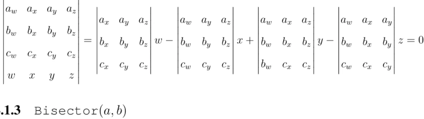
2 x+2 y+2 z+3 = 0. The normal vector of the plane has degree (2 , 2 , 2 ). This representation does not support orientation.which is the planea∨b∨c. The plane can be written as a determinant equation:
aw ax ay az
bw bx by bz
cw cx cy cz
w x y z
=
ax ay az
bx by bz
cx cy cz
w−
aw ay az
bw by bz
cw cy cz
x+
aw ax az
bw bx bz
bw cx cz
y−
aw ax ay
bw bx by
cw cx cy
z = 0
4.1.3
Bisector
(
a, b
)
a b Bab
Figure 4.3: Given point sites
a, b ∈ U the
construc-tion Bisector(a, b) pro-duces the perpendicular bi-sector ofab.
Thebisectorof distinct point sitesa, b∈U, depicted in Figure 4.3,
is the locus of points equidistant toaandb, and is the perpendicular bisector of segment ab. We sometimes write the bisector as Bab. When the two sites defining the bisector are subscripted, as in a1 anda2, we may abbreviate the bisector asB12.
We derive an expression forBab by observing that it is the set of points{q ∈R2 | kq−ak2 =kq−bk2}. Expanding this equation,
we get the standard and slope-intercept forms of the equation for
Bab as
standard form: 0 = 2(ax−bx)x+ 2(ay−by)y+b2x+b2y −a2x−a2y
slope-intercept form: y= (ax−bx) (by−ay)
x+1 2
b2
x+b2y −a2x−a2y
(by −ay) ,
Observe that writing just the degree of the coefficients, the standard from of the bisector is0 = 1
4.1.4
LineIntersection
(
`, h
)
`
h q
Figure 4.4: Given two non-parallel lines ` and h, in red,
LineIntersection(`, h)
constructs the coordinates of
q, in blue, the intersection point of`andh.
The construction LineIntersection(`, h) takes two distinct lines` andhand computes the homogeneous coordinates of their intersection pointq, as depicted in Figure 4.4. For Cartesian coor-dinates the output may be “parallel” rather than a point.
We warm up with lines in slope intercept form and then con-sider lines in standard form. Given lines ` : y = `mx +`b and
h : y = hmx+hb the coordinates of the intersection pointq of`
andhare
q = (`m−hm, hb−`b, `mhb−`bhm)
When `m = hm the two lines are parallel, thus qw = 0. When the coefficients of ` and h are degree 1, in Cartesian, thex-coordinate is degree 1 over 1 and they-coordinate is degree 2 over 1, or homogeneous coordinates, (
1 , 1 , 2 ). Many geometric algorithms analyzed with the Real-RAM model of computation have the property that processing left to right is the same as processing from top to bottom. However, as we will see in Section 4.2.1, this property does not always hold for lines in slope intercept form.Next we consider lines` and h, specified by homogeneous coordinates, i.e., ` = (`w, `x, `y).
The intersection pointqof the lines`andhis the solution to the linear equations
`xx+`yy+`w = 0
The solution gives us the homogeneous coordinates
q= (
`x `y hx hy ,− `w `y hw hy , `w `x hw hx ) (4.1)
Next, we analyze the polynomials of the output points for three specific forms of input lines. When`andhare degree 1, the lines have the form
1 x+ 1 y+ 1 . Their intersection has homogeneous coordinates of the form (2 , 2 , 2 ). When ` and h are defined by a pair of points, Section 4.1.1 says that they have the form 1 x+ 1 y+ 2 . Their intersection has ho-mogeneous coordinates of the form(2 , 3 , 3 ). When`is a degree 1 line and ahis defined by a pair of points their intersection has homogeneous coordinates of the form(2 , 3 , 3 ). When` andh are defined by two bisectors (described in Section 4.1.3) and the bisectors share a common defining point, the intersection is particularly important. It is the same as computing a vertex of the Voronoi diagram, which the topic of Chapter 7 and Chapter 8. Thus, we focus on constructing a Voronoi vertex in the next section.4.1.5
VoronoiVertex
(
a, b, c
)
b a c v Bab Bac
Figure 4.5: Given three non-collinear points a, b, c ∈ U,
in red, the construction
VoronoiVertex(a, b, c), constructs the coordinates of the point v which is equidistant toa,b, andc. AVoronoi vertexv, constructed from distinct pointsa, b, c ∈U, is
the point equidistant toa, b, andc, i.e., it is the center of the circle through a, b and c. As depicted in Figure 4.5 we can compute the coordinates of v by computing the intersection point of Bab
andBac. We derive the degree of a Voronoi vertex by combining the analysis on the degree of a bisector in Section 4.1.3 and line intersections in Section 4.1.4.
Let ` = Bab and h = Bac and recall that in Section 4.1.3 we
Byy +Bw =
1 x+ 1 y + 2 . Equation 4.1 gave the homogeneous coordinates of the intersection pointq, which, using degree notation, isq= (
1
1 1 1 ,− 2 1 2 1 , 2 1 2 1) = (
2 , 3 , 3 )Thus, each Cartesian coordinate of a Voronoi vertex is degree 3 over 2 or in homogeneous form
(
2 , 3 , 3 ).4.2
Predicates and Simple Algorithms
Next we derive the degrees of common predicates and simple algorithms used throughout this the-sis. We will no longer consider all possible point representations (e.g., point fromU, intersection point of two lines in standard form with degree 1 coordinates, etc.), but only those representations relevant in this thesis.
During implementation it is often convenient to use a perturbation scheme [3, 39, 41, 42, 114, 119] so that predicates are only positive or negative. In this section, we derive predicates with-out perturbation. Specific perturbation schemes are discussed in later sections in the context of specific algorithms.
4.2.1
PointOrdering
(
a, b
)
a b
Figure 4.6: The point a pre-cedes the pointb.
We compare two distinct points aandb by lexicographic order of their Cartesian coordinates. The pointa≺bif and only ifax < bx
(aw, bw > 0 or aw, bw < 0), we determine the ordering by clearing fractions and subtracting to get the predicates OrderX(aw, ax, bw, bx) = sign(awbx −axbw)and OrderY(aw, ay, bw, by) = sign(awby−aybw).
We can rewrite the degrees ofOrderandOrderYas
deg(OrderX(aw, ax, bw, bx)) = max{deg(aw) + deg(bx),deg(ax) + deg(bw)}
deg(OrderY(aw, ay, bw, by)) = max{deg(aw) + deg(by),deg(ay) + deg(bw)}.
We determine the degree for four cases by plugging coordinates into the equations above. First, ordering two points inUis degree 1 since points ofUhave coordinates of degree(
0 , 1 , 1 ). Second, ordering the intersection points of two pairs of lines in standard form with degree 1 coeffi-cients is degree 4 since the intersection points have coordinates of degree(2 , 2 , 2 ). Third, ordering a point ofUand a Voronoi vertex is degree 3 since Voronoi vertices have coordinates of degree(2 , 3 , 3 ). Fourth, ordering two Voronoi vertices is degree 5.Points described in the previous paragraph have the same degree for theirx- andy-coordinates; asymmetric pointshave Cartesian coordinates of different degrees. For example, the intersection of two lines in slope-intercept form, y =
1 x+ 1 , has coordinates of degree(1 , 1 , 2 ). We can order the x-coordinate with degree 2, but the y-coordinate is degree 3. We will see in Chapter 6 that asymmetric points may lead us to select one sweep direction over another or one decomposition direction over another.4.2.2
Orientation
(
a, b, q
)
qa b
Figure 4.7: The path from a
to b to q forms a right turn Given three distinct pointsa, b, q we determine if the straight line
two pointsa = (aw, ax, ay)andb = (bw, bx, by), we constructed an oriented line a∨b. Using the line fromatobwe can derive the predicate by plugging in the coordinates ofq= (qw, qx, qy)
Orientation(a, b, q) = sign(
aw ax ay
bw bx by
qw qx qy
)
= sign (axby−aybx)−(awby−bway)qx+ (awbx−bwax)qy
.
When all three points have positive spin (aw, bw, qw > 0), we can interpret the positive, neg-ative, and zero as path from a to b to q taking a left turn, right turn, and following a straight line, respectively.
Next, we analyze the polynomial for combinations of input points. When a, b, q ∈ U the
points have the coordinate degree(
0 , 1 , 1 ), and the predicate is degree 2. When one point is a Voronoi vertex, Section 4.1.5 says that it has coordinates degree (2 , 3 , 3 ), and the predicate is degree 4. In fact, the degree goes up by 2 for each Voronoi vertex: it takes degree 6 to determine the orientation of a point inUrelative to a segment between two Voronoi vertices and degree 8 to determine orientation for three arbitrary Voronoi vertices.4.2.3
Closer
(
a, b, q
)
Given three distinct pointsa, b, q ∈Uwe can test if a query pointqis closer toaorbwith degree 2
by comparing squared distances of Cartesian coordinates,
sign(kq−ak2
− kq−bk2
4.2.4
SideOfABisector
(
B
ab, q
)
q
a b Bab
Figure 4.8: The query pointq
is on the same side of theBab
asb. Recall from Section 4.1.3 that the bisector of two distinct points
a, b ∈ U, written Bab, is the locus of points equidistant to a
and b. Bisector Bab partitions the points of U into points on the same side as a, same side as b, and points on Bab. The predi-cateSideOfABisector(Bab, q)returns the partition containing a query pointq. In Figure 4.8 the query pointqis on the same side ofBabasb.
Since the points on the same side asaare closer toaand on the
same side asb are closer tob, we can use the same predicate asCloserand reinterpret the sign. Therefore,SideOfABisectoris degree 2.
4.2.5
OrderOnLine
(
B
ab, B
cd, `
)
a b Bab
d c
Bcd `
p q
Figure 4.9: The bisector Bab
is above the bisector Bcd on the line`.
Two non-vertical bisectors Bab andBcd intersect the vertical line
` : x = l withBab above, below or at the same point asBcd on`. In Figure 4.9, the lineBab is above the lineBcd on the vertical line `. We determine the ordering of Bab and Bcd on ` by comparing
y-coordinates of the intersection ofBabandBcdwith`.
Let q be the intersection of Bab and`. By plugging l into the slope-intercept form ofBab, derived in Section 4.1.3, we get that
qy = a2
x+a2y + 2lax−b2x−b2y−2lbx
2(by−ay) = 2
1
.4.2.6
OrderOnLine
(
g, h, `
)
g h ` q pFigure 4.10: The intersection of g and` is left of the inter-section ofhand`.
For three distinct lines in slope-intercept formg : y = gmx+gb
andh:y=hmx+hb, and`:y=`mx+`bsuch thatgm 6=`m and
hm 6=`m, letq=g∩`andp=h∩`. We determine ifqis to the left of, right of or incident topby comparing thex-coordinates ofpand
q. In Figure 4.10, h∩`is left ofg ∩`. Recall from Section 4.1.4
that px andqx are rational coordinates of degree 1 over 1. Thus, the polynomial is degree 2. In Section 4.2.1, we saw ordering the
y-coordinates of degree 1 lines in slope-intercept form is degree 3,
thus, we avoid it.
4.2.7
InCircle
(
a, b, c, q
)
q a
b
c
Figure 4.11: The query point
qin inside the circumcircle of
a,bandc. Given three non-collinear sites,a, b, c∈Uand a query pointqalso
inU, InCircle determines whetherqis inside the circumcircle of a, b, c ∈ U. In Figure 4.11, the query pointq is inside the
cir-cumcircle of a, b, and c. This could be done by comparing the squared distances from VoronoiVertex(a, b, c) to a and to q, which gives a degree 6 polynomial when you clear fractions, but that polynomial factors to give the degree 4 determinant,
1 ax ay a2
x+a2y
1 bx by b2
x+b2y
1 cx cy c2
x+c2y
1 qx qy q2
x+q2y
= 0
1 1 20
1 1 20
1 1 20
1 1 2
One may wonder if this polynomial can in fact be factored further. We see in Section 5.10 that in fact it cannot; it is irreducible.
Another way to arrive at this predicate is to consider the lifting map M : R2 → R3 with
M(x, y) = (x, y, x2 +y2). The three lifted pointsa0 =M(a),b0 =M(b)andc0 = M(c)lie on a
planeP inR3 that intersects the paraboloidQ:x2+y2−z = 0. The intersection curve ofP and
Qprojects down onto thexy-plane as the circle thougha,bandc; the points inside the circle lift to
one side ofP and the points outside lift to the other. Thus, an alternate way to derive this predicate is to writeP as described in Section 4.1.2. Plugging in the lifted pointq0
into the equation ofP
arrives at the same predicate.
4.2.8
IntersectInterior
(
ac, bd
)
a
d b
c
Figure 4.12: The interior of segmentsacandbdintersect. In Chapter 3 we saw two algorithms for determining if segments
intersect, assuming that no three points were collinear. Here, I describe a degree 2 algorithm for checking if the interior of the segments intersect without the non-collinearity assumption.
Given segmentsacandbdwith endpoints inU, and a 6=cand
b 6=d, the intersection of the interiors of the segments is empty, a point, or an open segment. Recall that when no three points defin-ing segments are collinear we can determine if the interiors of two
segments intersect by checking if the endpoints ofbdare on opposite sides of←ac→and the endpoints ofac are on opposite sides of←bd→. The checks use Orientation, the degree 2 predicate from Section 4.2.2.
To handle collinear points we one additional predicate. Given a segmentrsand a query point