REGION HOMOGENEITY IN THE LOGARITHMIC IMAGE PROCESSING FRAMEWORK: APPLICATION TO REGION GROWING ALGORITHMS

Image Anal Stereol 2019;38:43-52

Original Research Paper doi:10.5566/ias.2038

REGION HOMOGENEITY IN THE LOGARITHMIC IMAGE PROCESSING

FRAMEWORK: APPLICATION TO REGION GROWING ALGORITHMS

Guillaume Noyel

_{, Michel Jourlin}

1_{International Prevention Research Institute, Lyon , France,} 2_{University of Strathclyde Institute of Global} Public Health, Dardilly - Lyon Ouest, France, 3_{Laboratoire Hubert Curien, UMR CNRS 5516, Université Jean} Monnet, Saint-Etienne, France

e-mail: [email protected], [email protected]

(Received October 30, 2018; revised March 1, 2019; accepted March 14, 2019) Submitted to Image Anal Stereol, 10 pages

Original Research Paper

REGION HOMOGENEITY IN THE LOGARITHMIC IMAGE PROCESSING

FRAMEWORK: APPLICATION TO REGION GROWING ALGORITHMS

G

N

M

J

1_{International Prevention Research Institute, Lyon , France,}2_{University of Strathclyde Institute of Global Public}

Health, Dardilly - Lyon Ouest, France,3_{Laboratoire Hubert Curien, UMR CNRS 5516, Université Jean Monnet,}

Saint-Etienne, France

e-mail: [email protected], [email protected] (Submitted)

ABSTRACT

In order to create an image segmentation method robust to lighting changes, two novel homogeneity criteria of an image region were studied. Both were defined using the Logarithmic Image Processing (LIP) framework whose laws model lighting changes. The first criterion estimates the LIP-additive homogeneity and is based on the LIP-additive law. It is theoretically insensitive to lighting changes caused by variations of the camera exposure-time or source intensity. The second, the LIP-multiplicative homogeneity criterion, is based on the LIP-multiplicative law and is insensitive to changes due to variations of the object thickness or opacity. Each criterion is then applied in Revol and Jourlin’s (1997) region growing method which is based on the homogeneity of an image region. The region growing method becomes therefore robust to the lighting changes specific to each criterion. Experiments on simulated and on real images presenting lighting variations prove the robustness of the criteria to those variations. Compared to a state-of the art method based on the image component-tree, ours is more robust. These results open the way to numerous applications where the lighting is uncontrolled or partially controlled.

Keywords: Homogeneity of an image region, Image segmentation, Logarithmic Image Processing, Region Growing, Robustness to lighting changes.

INTRODUCTION

Segmentation of images acquired with different lighting conditions is a challenging task in image analysis that can occur in many settings such as visual inspection for industry (Cord et al., 2010; Noyel, 2011; Noyel et al., 2013; Parra-Denis et al., 2011), medical images (Noyel et al., 2014; 2017), security (Foresti et al., 2005), driving assistance (Hautière et al., 2006), etc. Lighting variations obviously represent a substantial obstacle for the development of reliable image processing algorithms. To overcome this difficulty, we can determine the two following approaches:

(i) Firstly, a practical approach consisting of circumventing the problem, e.g. by a learning process. This is often the case for face recognition, where a database is created by varying together the acquisition angle and the intensity of the lighting source (Ramaiah et al., 2015). An alternative way to learning processes aims at extracting from images some characteristics independent of lighting conditions (Wang et al., 2004; Shah et al., 2015). Another alternative aims at attenuating the lighting variations effects by means

of various methods like shadow suppression (Zhang et al., 2019).

shape spaces of Xu et al. (2016) is also theoretically invariant to those contrast changes.

Nevertheless, only a few papers focus on the causes of lighting variations. For this purpose, Jourlin and Noyel (2018) have defined two new homogeneity criteria in the LIP (Logarithmic Image Processing) framework, namely the LIP-additive and LIP-multiplicative homogeneity criteria. Each criterion is based either on the LIP law of addition+++

of two images or the multiplication××× of an image by

a scalar. Such laws are now well-known to model the lighting variations affecting the image acquisition step (Jourlin, 2016). The LIP-additive law +++ especially

models changes of source intensity or exposure-time whereas the LIP-multiplicative law ××× models the

thickness (or opacity) changes of the observed object. The aim of this paper is to study these homogeneity criteria in details. At the theoretical level, we will demonstrate their insensitivity to the lighting variations which are modelled by the corresponding LIP-laws. At the application level, we will prove their robustness to lighting changes on both simulated and on real images. For segmentation purpose we will apply them within the Revol and Jourlin’s (1997) algorithm which is in the class of Region Growing methods. This algorithm has the specificity of evaluating the homogeneity of an image region at each step. Its segmentation results will be compared to those obtained by the component-tree method of Passat et al.(2011).

MATERIALS AND METHODS

In this section, we will present the theoretical methods and their validation by the experimental material. First, we will summarise the Logarithmic Image Processing model. Second, we will present the specific lighting variations which are modelled by each LIP law. Third, we will introduce the LIP-additive and LIP-multiplicative homogeneity criteria. Fourth, we will recall the Revol and Jourlin’s (1997) region growing algorithm based on the homogeneity of an image region. Fifth, for comparison purpose, we will recall the sate-of-the-art method of Passatet al.(2011). Finally, we will present the experimental validation with simulated and real images.

LOGARITHMIC IMAGE PROCESSING

Introduced by Jourlin and Pinoli (1988; 2001), the LIP model possesses strong physical properties. Let f andgbe two grey level functions defined on the spatial support D⊂Rn, with values in the grey scale [0,M[

whereM∈R. In fact, the addition f+++gof fandgand

the scalar multiplicationλ××× fof fby a real numberλ

are both deduced from the opticalTransmittance Law according to:

f+++ g= f+g−f g/M, (1)

λ××× f=M−M(1−f/M)λ. (2)

Let us note that in the LIP framework, the grey scale[0,M[is inverted in comparison with the classical

one. Indeed, due to the transmittance law, 0 represents the “white” extremity of the scale, which corresponds to the observation of the source intensity. The reason of such an inversion is that 0 appears as the neutral element of the addition +++, i.e. when no obstacle is

placed between the source and the sensor.

From equation 1, the subtraction between two grey level functions is easily deduced:

f−−− g= f−g

1−_Mg . (3)

Remark. f −−− g can take negative values except for

f(x) _≥ g(x) at each point x. In such a case, the

subtraction f −−− g is a grey level image and the

difference f(x)−−− g(x) represents the Logarithmic

Additive Contrast between the grey levels f(x) and g(x)(Jourlin and Pinoli, 2001). This difference is the

grey level which must be added to the brightest one (here g(x)) in order to obtain the darkest one (here

f(x)).

Remark. Let us note that for 8-bit digitised images,M is equal to 256 and the grey levels vary from 0 to 255.

At the mathematical level, it has been demonstrated (Jourlin and Pinoli, 2001) that the laws

+++ and ××× give a Vector Space structure to the set

I(D,[0,M[) of images defined on a same spatial

supportD. This allows the use of many mathematical tools specific to this kind of space. In order to complete the outstanding properties of the LIP Model, let us recall that Brailean et al. (1991) have established its consistency with the Human Visual System, which opens the way to process images as a human eye would do.

WHICH LIGHTING VARIATIONS ARE MODELLED BY EACH LIP LAW?

Carre and Jourlin (2014) and Deshayes et al. (2015) have shown that the LIP-addition (respectively subtraction) of a constant to an image (resp. from an image) perfectly models a decrease (resp. an increase) of the camera exposure-time or of the source intensity. By definition of the scalar multiplicative law, the scalar

Image Anal Stereol 2019;38:43-52

Image Anal Stereol ?? (Please use\volume):1-10

a grey level image, one can associate to it a virtual half-transparent object producing f in transmission.

λ××× f represents then the image we would obtain by

stacking f on itselfλ times. The scalar multiplicative law models therefore the “opacity” changing of a half-transparent object or the thickness changing of a homogeneous object.

HOMOGENEITY CRITERIA: ADDITIVE HOMOGENEITY AND LIP-MULTIPLICATIVE HOMOGENEITY

Let f be a grey level function defined on the spatial supportD⊂Rn, with values in the grey scale

[0,M[ and consider a region R of D. There exist

some classical parameters evaluating the homogeneity of the image f in R, like the standard deviation

σf(R) or the “diameter” of R in the mathematical

sense defined by sup_x∈Rf(x)₋inf_x∈R f(x) which is

nothing but the dynamic of the image region. Such homogeneity parameters are obviously sensitive to lighting variations, which justifies the introduction of the two new criteria: the additive and the LIP-multiplicative homogeneity.

Remark. When there is no ambiguity, we will consider that the homogeneity of an image f over a region R is equivalent to the homogeneity of the region R. The region R is indeed supposed to be associated to the image f.

LIP-additive homogeneity

The homogeneityH+++

f (R)of the regionRis defined

as its dynamic in the LIP sense:

H+++

f (R) =sup x∈R f(x)

− −− inf

x∈Rf(x) (4)

Let us note thatH+++

f (R)lies in[0,M[and represents

thus a grey level which can be interpreted as the maximal Logarithmic Additive Contrast observed in the region (Jourlin and Pinoli, 2001).

The most important property of this homogeneity criterion is its insensitivity to exposure time variations modelled by LIP-addition/subtraction of a constantC:

H+++

f+++C(R) =H +++

f (R) (5)

Proof. Let us first remark that

sup

x∈R{(f

+ +

+ C)(x)}=sup

x∈R{f(x)}

+ + + C.

In fact, equation 1 gives:

sup{f} +++C=sup{f}+C−(C.sup{f})/M

= (1−C/M)sup{f}+C=sup{f(1−C/M)_}+C

=sup{f(1−C/M) +C}=sup{f+C−f.C/M}

=sup{f+++C}.

In the same way, we have: infx∈R{(f+++ C)(x)}=inf_x

∈R{f(x)} +++C.

In such conditions, equation 4 can be written: H+++

f+++C(R) = (sup

x∈R{f(x)}

+

++C)−−− (inf

x∈R{f(x)} +

+ +C).

The following computation shows that(A+++C)−−− (B+++

C)is equal toA−−− B:

(A+++C)−−− (B+++ C) =A

+C₋A_M.C₋B+C₋B_M.C

1−B+C−BM.C

M

= (A−B)

1−_MC

1−_MB −_MC −B_M.C2

= (A−B)

1−_MC

1−_MB1−_MC=

(A−B)

1−_MB

=A−−− B.

The two previous results prove equation 5.

LIP-multiplicative homogeneity

Now, we propose a homogeneity criterion based on the LIP scalar multiplication and more precisely on the notion of Logarithmic Multiplicative Contrast (LMC) (Jourlin et al., 2012). Let us recall that the LMC associated to a pair of grey levels g1 and g2,

whereg1andg2are strictly positive, is the real number

defined by the formula:

LMC(g₁,g₂)××× min(g₁,g₂) =max(g₁,g₂). (6)

In the context of images acquired in transmission, this means that the LMC of two grey levels represents the number of times the brightest of them must be stacked upon itself to get the darkest one. In such conditions, the LIP multiplicative homogeneity of a regionRis computed according to:

H×××

f (R) =LMC(sup

x∈R{f(x)},xinf∈R{f(x)}) (7)

= ln(1−supx∈R{f(x)}/M)

ln(1₋inf_x∈R{f(x)_}/M). (8)

Remark. In the case where infx∈R f(x) =0, one can

replace this value by 1 in order to avoid an infinite value forH×××

This homogeneity criterion possesses the fundamental property to be insensitive to variations of lighting modelled by the LIP-multiplicative law×××,

like opacity or thickness variations:

H×××

λ××× f(R) =H

×××

f (R). (9)

Proof. Suppose that H×××

f (R) = µ, which means that

sup_x∈Rf(x) =µ××× inf_x∈R f(x). We have to prove the

equality:

sup

x∈Rλ

×

×× f(x) =µ××× inf

x∈Rλ××× f(x). (10)

Givenλ≥0, it is easy to establish that:

sup

x∈R{λ

××× f(x)}=sup

x∈R{M(1−(1−f(x)/M) λ_)}

=M(1−inf

x∈R{(1−f(x)/M) λ_})

=M(1₋(inf

x∈R{1−f(x)/M}) λ₎

=M(1−(1−sup

x∈R{f(x)}/M) λ₎

=λ××× sup

x∈Rf(x).

In the same way, infx∈Rλ ××× f(x) = λ ×××

infx∈R f(x). Thus, equation 10 is established, which

ends the proof.

A REGION GROWING ALGORITHM BASED ON REGION HOMOGENEITY

Revol and Jourlin (1997) presented a region growing method which minimises the region variance. In the sequel, we propose to replace the variance by one of the homogeneity criteria H+++

or H×××

. Let us present the principles of this algorithm. The details are given in (Revol and Jourlin, 1997).

Let dynf(R) be the dynamic range of the image

f over the region R. It is defined by dynf(R) =

[min_x∈R{f(x)_},max_x∈R{f(x)_}].

At each stepn, a regionRn is dilated by a unitary

structuring element N, e.g a square of length side 3 pixels (Minkowski, 1903; Matheron, 1967; Serra and Cressie, 1982; Najman and Talbot, 2013). This gives a regionDn+1=Rn⊕N whose homogeneityHf(Dn+1)

is measured. Depending on a threshold value t, the region is considered as homogeneous or not.

1.If Hf(Dn+1) ≤ t, the region Dn+1 is then

considered as homogeneous. The new regionRn+1

becomesDn+1.

2.If Hf(Dn+1) > t, the region Dn+1 is then

inhomogeneous. AreductionprocessRdctf(Dn+1)

truncates the extremal classes of the histogram ofDn+1 by keeping only the pixels belonging to

the dynamic range of Rn, dynf(Rdctf(Dn+1)) =

dynf(Rn). This gives a regionD_n+1.

2.a If Hf(Dn+1) ≤ t, the region Dn+1 is then

modified by an extension process which adds the neighbouring pixels to the region according to both following conditions. i) The new pixel values have a LIP-difference less or equal than 1 with the maximum or the minimum values of f over D

n+1. ii) The new pixels give an

homogeneous region. The new region Rn+1

becomes the extension ofD

n+1:E(Dn+1).

2.b IfHf(Dn+1)>t, acontractionprocess reduces

the dynamic range of the region D n+1 by

removing the extremal classes of its histogram until the region becomes homogeneous. LIP-addition and LIP-subtraction replace the classical addition and subtraction used by Revol and Jourlin (1997). The new regionRn+1 is the

contraction ofD

n+1:Ctrct(Dn+1).

The algorithm stops when the region Rn+1 does not

grow any more.

For a fully automatic segmentation method, the seed points could be chosen as the minima of a function such as: a gradient of the image - like for the watershed transform (Beucher and Meyer, 1992) - or a map of Asplund’s distances of the image (Jourlinet al., 2012; 2014; Noyel and Jourlin, 2015; 2017b;a). The seed points could also be automatically determined by a previous classification (Noyelet al., 2007; 2010; 2014). As the homogeneity criterion is invariant to contrast changes with an optical cause, the threshold could be learnt from a training database (Lu et al., 2017). It could also be automatically chosen as the most frequent contrast on every pixel neighbourhoods (Jourlin, 2016).

A STATE OF THE ART METHOD BASED ON THE IMAGE COMPONENT-TREE

Our method will be compared to the state-of-the-art one of Passat et al. (2011) which is based on level sets and presents a certain robustness to lighting variations. It consists of an interactive segmentation by component-tree. A component-tree is the tree formed by the inclusion relation between the binary components of the successive image level sets. A node This homogeneity criterion possesses the

fundamental property to be insensitive to variations of lighting modelled by the LIP-multiplicative law×××,

like opacity or thickness variations:

H×××

λ×××f(R) =H

×××

f (R). (9)

Proof. Suppose that H×××

f (R) = µ, which means that

sup_x∈R f(x) =µ××× inf_x∈Rf(x). We have to prove the

equality:

sup

x∈Rλ

× ×

× f(x) =µ××× inf

x∈Rλ××× f(x). (10)

Givenλ ≥0, it is easy to establish that:

sup

x∈R{λ

× ×

× f(x)}=sup

x∈R{M(1−(1−f(x)/M) λ_)}

=M(1₋inf

x∈R{(1−f(x)/M) λ_})

=M(1−(inf

x∈R{1−f(x)/M}) λ₎

=M(1₋(1₋sup

x∈R{f(x)}/M) λ₎

=λ××× sup

x∈R f(x).

In the same way, infx∈Rλ ××× f(x) = λ ×××

infx∈Rf(x). Thus, equation 10 is established, which

ends the proof.

A REGION GROWING ALGORITHM BASED ON REGION HOMOGENEITY

Revol and Jourlin (1997) presented a region growing method which minimises the region variance. In the sequel, we propose to replace the variance by one of the homogeneity criteria H+++

or H×××

. Let us present the principles of this algorithm. The details are given in (Revol and Jourlin, 1997).

Let dynf(R) be the dynamic range of the image

f over the region R. It is defined by dynf(R) =

[min_x∈R{f(x)_},max_x∈R{f(x)_}].

At each stepn, a regionRnis dilated by a unitary

structuring element N, e.g a square of length side 3 pixels (Minkowski, 1903; Matheron, 1967; Serra and Cressie, 1982; Najman and Talbot, 2013). This gives a regionDn+1=Rn⊕Nwhose homogeneityHf(Dn+1)

is measured. Depending on a threshold value t, the region is considered as homogeneous or not.

1.If Hf(Dn+1) ≤ t, the region Dn+1 is then

considered as homogeneous. The new regionRn+1

becomesDn+1.

2.If Hf(Dn+1) > t, the region Dn+1 is then

inhomogeneous. A reduction processRdctf(Dn+1)

truncates the extremal classes of the histogram of Dn+1 by keeping only the pixels belonging to

the dynamic range of Rn, dynf(Rdctf(Dn+1)) =

dynf(Rn). This gives a regionDn+1.

2.a If Hf(Dn+1) ≤ t, the region Dn+1 is then

modified by an extension process which adds the neighbouring pixels to the region according to both following conditions. i) The new pixel values have a LIP-difference less or equal than 1 with the maximum or the minimum values of f over D

n+1. ii) The new pixels give an

homogeneous region. The new region Rn+1

becomes the extension ofD

n+1:E(Dn+1).

2.b IfHf(Dn+1)>t, acontractionprocess reduces

the dynamic range of the region D n+1 by

removing the extremal classes of its histogram until the region becomes homogeneous. LIP-addition and LIP-subtraction replace the classical addition and subtraction used by Revol and Jourlin (1997). The new regionRn+1is the

contraction ofD

n+1:Ctrct(Dn+1).

The algorithm stops when the region Rn+1 does not

grow any more.

For a fully automatic segmentation method, the seed points could be chosen as the minima of a function such as: a gradient - like for the watershed transform (Beucher and Meyer, 1992) - or a map of Asplund’s distances (Jourlin et al., 2012; 2014; Noyel and Jourlin, 2015; 2017b;a). The seed points could also be automatically determined by a previous classification (Noyel et al., 2007; 2010). As the homogeneity criterion is invariant to contrast changes with an optical cause, the threshold could be learnt from a training database (Luet al., 2017). It could also be automatically chosen as the most frequent contrast on every pixel neighbourhoods (Jourlin, 2016).

A STATE OF THE ART METHOD BASED ON THE IMAGE COMPONENT-TREE

Image Anal Stereol 2019;38:43-52

Image Anal Stereol ?? (Please use\volume):1-10

of the image level set Xv(f) = {x ∈ D|f(x) ≥ v}.

Let K be the set of all connected components of

all level sets. The subset K _⊂K of the connected

components which best fits the user selected region G inD is automatically determined by the following minimisation problem:

K=arg min K_∈P(K){d

α_(∪N

∈KN,G)}.

P(K)is the set of the parts ofK. The pseudo-distance

dα is defined by

dα(X,Y) =α_|X_\Y_|+ (1₋α)_|Y_\X_|,

where α ∈[0,1]. d0(X,Y) =_|Y _\X_| and d1(X,Y) =

|X\Y|are respectively the amount of false-negatives and false-positives inX with respect toY. A solution to this minimisation problem can be found by dynamic programming. The details are given in (Passat et al., 2011). In the sequel, we have used the publicly available code of Naegel and Passat (2014).

EXPERIMENTAL VALIDATION

We have just established that the LIP-additive homogeneity criterion H+++

f (R) is theoretically

insensitive to a LIP-addition+++ or to a LIP-subtraction

−−− of a constant to or from an image, respectively.

These operations model the lighting changes caused by a variation of the source intensity or of the exposure-time of the camera. As for the LIP-multiplicative homogeneity criterion H×××

f (R), it is insensitive to a

LIP-multiplication of an image f by a scalar which models the variations of the object thickness or opacity. Let us perform an experimental validation of these insensitivities through simulated and real images. Let us also compare the presented approach to the state-of-the-art method of Passatet al.(2011).

Simulated images

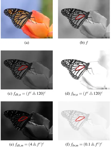
For this experiment, we have selected a colour image of a butterfly (Fig. 1a) from the dataset YFCC100M (Yahoo Flickr Creative Commons 100M) (Thomee et al., 2016; Butterfly, 2010). We have extracted its luminance as a grey-level image f (Fig. 1b). In order to verify the respective insensitivities of the criteria H+++

and H×××

to lighting variations simulated by a LIP-addition +++ or a

LIP-multiplication ×××, we have darkened and brightened

this luminance image f by using each of the LIP-operations.

For the LIP-additive homogeneity criterion H+++

f (R), a dark image fdk,a is obtained by a

LIP-addition of a constant k=120 to the complement fc

of the image f, fdk,a= (fc+++ k)c(Fig. 1c). The image

complement, which is defined by fc =M−1− f, allows to take advantage of the LIP-scale. A bright image fbr,a is also simulated by a LIP-subtraction of

the same constant: fbr,a= (fc−−− k)c(Fig. 1d).

For the LIP-multiplicative homogeneity criterion H×××

f (R), a dark image fdk,m is obtained by a

LIP-multiplication by a scalar λdr = 4 of the image

complement fc_{, f}

dk,m= (λdr××× fc)c(Fig. 1e). A bright

image fbr,m is also simulated by a LIP-multiplication

by a scalarλbr=0.1, fbr,m= (λbr××× fc)c(Fig. 1f).

In all these five images f, fdk,a fbr,a, fdk,mand fbr,m

the same regionRis selected. The homogeneity criteria H+++

and H×××

are then computed in the region R of the images f, fdk,a, fbr,a and of the images f, fdk,m,

fbr,m, respectively. Their values are given in section

“Results” (p. 6).

Real images

The robustness to lighting variations of the LIP-additive homogeneity criterion H+++

and of the LIP-multiplicative criterionH×××

needs to be verified on real images by using specific experimental material.

The LIP-additive homogeneity criterion H+++

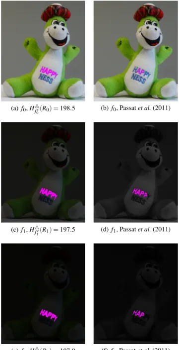
is expected to have a low sensitivity to variations of source intensity or exposure-time of the camera. In order to verify this assumption, we have conducted an experiment. An image of the same scene is acquired by a camera with significantly different exposure-times and slightly different positions. The scene is composed of a soft toy monster named “Nessie” (Fig. 2). Three colour images are captured with different exposure-times 1/40 s (Fig. 2a, 2b), 1/400 s (Fig. 2c, 2d) and 1/800 s (Fig. 2c, 2e). They are converted to luminance images in grey levels: f0, f1 and f2, respectively. The

shorter the exposure-time is, the darker the image becomes. A segmentation is performed by Revol and Jourlin’s (1997) algorithm using the LIP-additive homogeneity criterion H+++

and a threshold of 200 to decide if a region R is homogeneous (i.e. H+++

f (R)≤

200) or not. The initialisation of the algorithm is done by a seed point manually selected inside the letters on the body of “Nessie”. To take advantage of the LIP-scale, the segmentation is performed on the complement of the three luminance images fc

0, f1cand

fc

2. Three segmented regionsR0(Fig. 2a),R1(Fig. 2c)

andR2(Fig. 2e) are thereby obtained in the images f0,

f1and f2, respectively. The LIP-additive homogeneity

of those regions is then computed. For comparison purpose, Passat et al.’s (2011) segmentation method is applied to the images f0 (Fig. 2b), f1 (Fig. 2d) and

f2 (Fig. 2f). The user selected regionsGare the same

dilation by a square of length side 3 pixels. As the user selected regions G are much smaller than the letters that we want to segment, we choose a parameterα=0

in order to minimise the number of false-negatives d0_(∪N

∈KN,G)in those regionsG. After minimisation,

this number is equal to zero.

In order, to verify the low sensitivity to object opacity of the LIP-multiplicative homogeneity criterion H×××

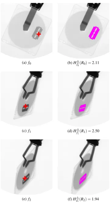
, we have selected three X-ray images of a luggage acquired under different exposures for security purpose (Fig. 3). The images are coming from a publicly available database, namely GDXray (Mery et al., 2015; GDXray, 2015). The object to be detected is a razor blade. Depending on its orientation, the x-rays pass through different thicknesses of the matter and are therefore more or less absorbed. In the first image f0 (Fig. 3a), the razor blade is perpendicular

to the x-rays coming from the source. The image of the razor blade is obviously brighter in this image f0

than in the two others f1 (Fig. 3c) and f2 (Fig. 3e)

where the razor blade is oblique to the x-rays. To detect this object, Revol and Jourlin’s (1997) segmentation approach is used with a threshold of 2.7 on the LIP-multiplicative homogeneity criterion H×××

of a region. The algorithm is initialised by manually selected seed points inside the razor blade (Fig. 3a, 3c and 3e). Three regions R0 (Fig. 3b), R1 (Fig. 3c) and R2

(Fig. 3e) corresponding to the object are then obtained in the images f0, f1 and f2, respectively. The

LIP-multiplicative homogeneity of those regions is then estimated. Its values are presented in the following section.

RESULTS

The experimental results are given for the simulated and the real images.

SIMULATED IMAGES

The LIP-additive homogeneity criterionH+++

of the region is computed for the image f (Fig. 1b), its darkened versionfdk,aby LIP-addition (Fig. 1c) and its

brightened version fbr,a by LIP-subtraction (Fig. 1d).

For each image, the criterion H+++

of the region R is equal to:

H+++

fc(R) =H_f+++c

dk,a(R) =H

+++ fc

br,a(R) =150.7. This result

verifies thereby the insensitivity of the LIP-additive homogeneity criterionH+++

to LIP-addition+++ or

LIP-subtraction −−− of a constant to or from an image,

respectively.

The LIP-multiplicative homogeneity criterionH×××

is also estimated in the image f (Fig. 1b) and

its darkened and brightened versions by LIP-multiplication fdk,m (Fig. 1e) and fbr,m (Fig. 1f),

respectively. For each image the criterionH×××

of the regionRis equal to:

H×××

fc(R) = H_f×××c

dk,m(R) = H

×××

fc

br,m(R) = 3.33. This result

shows the insensitivity of the LIP-multiplicative criterionH×××

to the LIP-multiplication××× of an image

by a scalar.

(a) (b)f

(c) fdk,a= (fc+++120)c (d)f_br,a= (fc−−−120)c

(e)fdk,m= (4××× fc)c (f) fbr_,m= (0.1××× fc)c

Fig. 1. (a) Colour image of a butterfly and (b) its luminance image f with a region R in red. (c) Darkened image fdk,a obtained by LIP-addition of a

constant k=120. (d) Brightened image fbr,aobtained

by LIP-subtraction of k. (e) Darkened image fdk,m

obtained by a LIP-multiplication of fc _{by λ} dr =

4. (f) Brightened image fbr,m obtained by a

LIP-multiplication byλbr=0.1.

REAL IMAGES

Let us give the results obtained on the real images of figures 2 and 3.

The LIP-additive homogeneity criterion H+++

is illustrated in figure 2. One can notice that the segmentations of the letters on the body of “Nessie” are very similar in all the three images f0 (Fig. 2a),

f1 (Fig. 2c) and f2 (Fig. 2e) using this criterion

H+++

Image Anal Stereol 2019;38:43-52

Image Anal Stereol ?? (Please use\volume):1-10

(i.e. our approach). In addition, the values of the homogeneity criterion are as follows: H+++

fc

0(R0) =

198.5, H+++

f₁c(R1) =197.5 and H + + +

f₂c(R2) =197.0. These

values are very close for the three regions R0, R1

and R2 of these images which were acquired with

significantly different exposure-times. Those results prove therefore the robustness of the LIP-additive homogeneity criterion H+++

in Revol and Jourlin’s (1997) segmentation method to the variations of the camera exposure-time. This approach is also compared to the one of Passat et al. (2011). One can notice that the segmentations with this latter method are different between the three images f0 (Fig. 2b), f1

(Fig. 2d) and f2 (Fig. 2f). Those results show that

Passat et al.’s (2011) method lacks of robustness for important variations of the camera exposure-time, whereas ours is robust to such variations. In addition, the letters are not entirely extracted with Passatet al.’s (2011) method whereas with ours, their segmentations are better (Fig. 2a, 2c and 2e).

Figure 3 presents the results obtained for the LIP-multiplicative criterion H×××

. The segmentations of the razor blade are very similar in the three images (Fig. 3b, 3d and 3f) using this criterion H××× within the Revol and Jourlin’s (1997) method.

As the three images were captured with different exposures, the x-rays were differently absorbed by the object. In addition, the values of the homogeneity criterion are the following for each segmented regions: H×××

fc

0(R0) = 2.11, H

×××

fc

1(R1) = 2.50 and H

×××

fc

2(R2) =

1.94. One can notice that the criterion values are

of similar amplitudes for the three regions of an object presenting different thicknesses which absorb the x-rays. This experiment illustrates the robustness of the LIP-multiplicative criterion H×××

in Revol and Jourlin’s (1997) segmentation method to different object opacities (or absorptions).

DISCUSSION

The results obtained with the simulated images show that the LIP-additive homogeneity criterion H+++

is insensitive to the LIP-addition +++ or the

LIP-subtraction −−− of the image complement fc

by a constant. These operations +++ and −−− model

a darkening or a brightening of the image by a variation of the source intensity or the exposure-time of the camera (Jourlin, 2016). This result proves the theoretical insensitivity of the LIP-additive criterion H+++

to such variations. Similarly, the LIP-multiplicative homogeneity criterion H×××

is theoretically insensitive to the variations of the object

opacity or thickness which are modelled by a LIP-multiplication××× by a scalar (Jourlin, 2016).

(a)f₀,H+++

fc

0(R0) =198.5 (b)f0, Passatet al.(2011)

(c)f1,Hf+++c

1(R1) =197.5 (d)f1, Passatet al.(2011)

(e)f2,Hf+++c

2(R2) =197.0 (f) f2, Passatet al.(2011)

Fig. 2.Comparison of the robustness to three exposure-time variations (a, c, e) of Revol and Jourlin’s (1997) method with a LIP-additive homogeneity criterion H+++

and (b, d, f) of Passat et al.’s (2011) method. Colour versions of the luminance images (a, b) f0,

(c, d) f1 and (e, f) f2 acquired at 1/40 s, 1/400 s

and 1/800 s, respectively. The segmented regions are depicted in magenta colour. The homogeneity criterion values H+++

f₀c(R0), H + + +

f₁c(R1), H + + +

f₂c(R2) of the regions R0,

R1 and R2are given under the images (a), (c) and (e),

(a)f0 (b)H×××

fc

0(R0) =2.11

(c)f1 (d)H×××

fc

1(R1) =2.50

(e)f2 (f)H×××

fc

2(R2) =1.94

Fig. 3. Robustness to variations of object opacity of the segmentation by LIP-multiplicative homogeneity criterion H×××

. (a) (b) and (c) Three images f0, f1

and f2 acquired for different exposures of a luggage

containing a razor blade. The seed points are shown by a red cross. (d) (e) and (f). The segmented regions R0, R1and R2of the images f0, f1and f2, respectively,

are shown in magenta colour. The values of the homogeneity criteria H×××

fc

0(R0), H

×××

fc

1(R1), H

×××

fc

2(R2) are

given under the images (b), (d) and (f).

These simulations are confirmed by the experimental results. Figure 2 proves the robustness of the LIP-additive homogeneity criterion H+++

f (R) to

lighting changes caused by a variation of an exposure-time of the camera. This lighting variation is equivalent to a variation of the source intensity. Although the methods based on levels sets are theoretically robust to a contrast change caused by a continuous

and increasing function applied to the image, the results obtained in figure 2 prove that the level set approach of Passat et al. (2011) lacks of robustness for important variations of the camera exposure-time. The results given in figure 3 prove the robustness of the LIP-multiplicative homogeneity criterion H×××

f (R)

to lighting changes caused by variations of the object opacity.

The previous results show that the level sets methods based on component-trees (Salembier et al., 1998; Passat et al., 2011) or on inclusion trees (Monasse and Guichard, 2000; Xu et al., 2016) will therefore strengthen their robustness to strong contrast changes - due to an optical cause - by using a LIP homogeneity criterion. The optical cause can either be a variation of the source intensity, which will be corrected by the LIP-additive criterion H+++

, or a variation of the object opacity, which will be corrected by the LIP-multiplicative criterionH×××

. These findings will be studied in a future paper.

CONCLUSION

We have therefore successfully introduced two new region homogeneity criteria which are robust to lighting changes, namely the LIP-additive homogeneity criterionH+++

and the LIP-multiplicative criterionH×××

. With experiments on simulated and on real images, we have shown that the LIP-additive homogeneity criterionH+++

is robust to changes caused by variations of source intensity (or exposure-time of the camera) whereas the LIP-multiplicative criterion H×××

is robust to changes due to variations of object opacity (or thickness). The introduction of those criteria in Revol and Jourlin’s (1997) segmentation method gives it the same robustness. Compared to Passatet al.’s (2011) method based on the component-tree of the image level sets, ours is more robust to strong intensity changes due to one of the previous optical cause. As far as we know, this is the first time that a segmentation method based on a region homogeneity parameter robust to those type of lighting changes has been shown. This novel method of segmentation paves the way to numerous applications presenting strong lighting variations.

ACKNOWLEDGEMENTS

Image Anal Stereol 2019;38:43-52

Image Anal Stereol ?? (Please use\volume):1-10

REFERENCES

Beucher S, Meyer F (1992). The morphological approach to segmentation: The watershed transformation, vol. 34 of Optical Engineering, chap. 12. Marcel Dekker, New York, 433–481. Brailean J, Sullivan B, Chen C, Giger M (1991).

Evaluating the EM algorithm for image processing using a human visual fidelity criterion. In: Int Conf Acoust Spee, vol. 4.

Butterfly (2010). Butterfly image from the YFCC100M dataset. http://www. flickr.com/photos/45563311@N04/

4350683057/. Licence CC BY-NC-SA 2.0.

Carre M, Jourlin M (2014). LIP operators: Simulating exposure variations to perform algorithms independent of lighting conditions. In: 2014 International Conference on Multimedia Computing and Syst. (ICMCS). IEEE.

Chen T, Yin W, Zhou XS, Comaniciu D, Huang TS (2006). Total variation models for variable lighting face recognition. IEEE T Pattern Anal 28:1519– 24.

Cord A, Bach F, Jeulin D (2010). Texture classification by statistical learning from morphological image processing: application to metallic surfaces. J Microsc Oxford UK 239:159–66.

Deshayes V, Guilbert P, Jourlin M (2015). How simulating exposure time variations in the LIP model. Application: moving objects acquisition. In: Acta Stereol., Proc. 14th ICSIA.

Elad M, Kimmel R, Shaked D, Keshet R (2003). Reduced complexity retinex algorithm via the variational approach. J Vis Commun Image R 14:369 – 388.

Foresti GL, Micheloni C, Snidaro L, Remagnino P, Ellis T (2005). Active video-based surveillance system: the low-level image and video processing techniques needed for implementation. IEEE Signal Proc Mag 22:25–37.

GDXray (2015). Database of x-ray images.

http://dmery.ing.puc.cl/index.

php/material/gdxray/. Set of baggage

images no. B0063, image no. 3, 10, 11. Accessed 16th_{October 2018.}

Hautière N, Aubert D, Jourlin M (2006). Measurement of local contrast in images, application to the measurement of visibility distance through use of an onboard camera. Trait Signal 23:145–58. Jourlin M (2016). Logarithmic Image Processing:

Theory and Applications, vol. 195 of Adv Imag Elect Phys. Elsevier Science.

Jourlin M, Carré M, Breugnot J, Bouabdellah M (2012). Chapter 7 - Logarithmic Image Processing: Additive contrast, multiplicative contrast, and associated metrics. In: Hawkes PW, ed., Adv Imag Elect Phys, vol. 171. Elsevier, 357 – 406.

Jourlin M, Couka E, Abdallah B, Corvo J, Breugnot J (2014). Asplünd’s metric defined in the Logarithmic Image Processing (LIP) framework: A new way to perform double-sided image probing for non-linear grayscale pattern matching. Pattern Recogn 47:2908 – 2924.

Jourlin M, Noyel G (2018). Homogeneity of a region in the Logarithmic Image Processing framework: application to region growing algorithms. In: Willot F, Forest S, eds., Physics and Mechanics of Random Structures: from Morphology to Material Properties. Ile d’Oléron, France: Presse des Mines.

https://hal.archives-ouvertes.fr/

hal-01822522.

Jourlin M, Pinoli J (1988). A model for logarithmic image processing. J Microsc Oxford UK 149:21– 35.

Jourlin M, Pinoli J (2001). Logarithmic image processing: The mathematical and physical framework for the representation and processing of transmitted images. In: Hawkes PW, ed., Adv Imag Elect Phys, vol. 115. Elsevier, 129 – 196. Lu L, Zheng Y, Carneiro G, Yang L, eds. (2017). Deep

Learning and Convolutional Neural Networks for Medical Image Computing - Precision Medicine, High Performance and Large-Scale Datasets. Advances in Computer Vision and Pattern Recognition. Springer.

Matheron G (1967). Eléments pour une théorie des milieux poreux. Masson, Paris.

Mery D, Riffo V, Zscherpel U, Mondragón G, Lillo I, Zuccar I, Lobel H, Carrasco M (2015). GDXray: The database of X-ray images for nondestructive testing. J Nondestruct Eval 34:42.

Minkowski H (1903). Volumen und oberfläche. Mathematische Annalen 57:447–95.

Monasse P, Guichard F (2000). Fast computation of a contrast-invariant image representation. IEEE T Image Process 9:860–72.

Naegel B, Passat N (2014). Interactive Segmentation Based on Component-trees. Image Processing On Line 4:89–97.

Najman L, Talbot H (2013). Mathematical Morphology: From Theory to Applications. Wiley-Blackwell, 1st ed.

https://patentscope.wipo.int/

search/en/WO2011131410. International

PCT patent WO2011131410 (A1). Also published as: US9002093 (B2), FR2959046 (B1), JP5779232 (B2), EP2561479 (A1), CN102844791 (B), BR112012025402 (A2).

Noyel G, Angulo J, Jeulin D (2007). Morphological segmentation of hyperspectral images. Image Anal Stereol 26:101–9.

Noyel G, Angulo J, Jeulin D (2010). A new spatio-spectral morphological segmentation for multi-spectral remote-sensing images. Int J Remote Sens 31:5895–920.

Noyel G, Angulo J, Jeulin D, Balvay D, Cuenod CA (2014). Multivariate mathematical morphology for DCE-MRI image analysis in angiogenesis studies. Image Anal Stereol 34:1–25.

Noyel G, Jeulin D, Parra-Denis E, Bilodeau M (2013). Method of checking the appearance of the surface of a tyre. https://patentscope.

wipo.int/search/en/WO2013045593.

International PCT patent WO2013045593 (A1), also published as US9189841 (B2), FR2980735 (B1), EP2761587 (A1), CN103843034 (A). Noyel G, Jourlin M (2015). Asplund’s metric

defined in the logarithmic image processing (LIP) framework for colour and multivariate images. In: 2015 IEEE Int. Conf. on Image Process.

Noyel G, Jourlin M (2017a). Double-sided probing by map of Asplund’s distances using logarithmic image processing in the framework of mathematical morphology. In: Lect Notes Comput Sc. Cham: Springer Int. Publishing.

Noyel G, Jourlin M (2017b). Spatio-colour Asplünd’s metric and logarithmic image processing for colour images (LIPC). In: Lect Notes Comput Sc, vol. 10125. Cham: Springer Int. Publishing. Noyel G, Thomas R, Bhakta G, Crowder A, Owens D,

Boyle P (2017). Superimposition of eye fundus images for longitudinal analysis from large public health databases. Biomed Phys Eng Express 3:045015.

Parra-Denis E, Bilodeau M, Jeulin D (2011). Multistep detection of oriented structure in complex textures. In: International Congress for Stereology. Beijing, China.

Passat N, Naegel B, Rousseau F, Koob M, Dietemann JL (2011). Interactive segmentation based on component-trees. Pattern Recogn 44:2539 – 2554. Semi-Supervised Learning for Visual Content Analysis and Understanding.

Ramaiah NP, Ijjina EP, Mohan CK (2015). Illumination invariant face recognition using convolutional neural networks. In: 2015 IEEE International Conference on Signal Processing, Informatics, Communication and Energy Systems (SPICES).

Revol C, Jourlin M (1997). A new minimum variance region growing algorithm for image segmentation. Pattern Recogn Lett 18:249 – 258.

Salembier P, Oliveras A, Garrido L (1998). Antiextensive connected operators for image and sequence processing. IEEE T Image Process 7:555–70.

Serra J, Cressie N (1982). Image analysis and mathematical morphology, vol. 1. Academic Press, London.

Shah JH, Sharif M, Raza M, Murtaza M, Saeed-Ur-Rehman (2015). Robust face recognition technique under varying illumination. J Appl Res Technol 13:97 – 105.

Thomee B, Shamma DA, Friedland G, Elizalde B, Ni K, Poland D, Borth D, Li LJ (2016). YFCC100M: The new data in multimedia research. Commun ACM 59:64–73.

Wang H, Li SZ, Wang Y (2004). Face recognition under varying lighting conditions using self quotient image. In: Sixth IEEE International Conference on Automatic Face and Gesture Recognition, 2004. Proceedings.

Xu Y, Géraud T, Najman L (2016). Connected filtering on tree-based shape-spaces. IEEE T Pattern Anal 38:1126–40.

Yu H, Fan J (2017). A novel segmentation method for uneven lighting image with noise injection based on non-local spatial information and intuitionistic fuzzy entropy. EURASIP J Adv Sig Pr 2017:74. Zhang W, Zhao X, Morvan J, Chen L (2019).