Relative Response Array: A New Tool for Control
Configuration Selection
Amit Jain and B. V. Babu
Abstract—This paper is an attempt to overcome the limitations associated with a dynamic measure of process interaction the “Relative Response Array (RRA)”. The RRA was originally proposed for 2 ×2 plant models only. Through this paper we are proposing the four different versions of the RRA to make it a more generalized measure of closed-loop interaction. They are defined based on open and closed-loop step response of the plant model elements using controller-independent and controller-approach. To show the applicability of the proposed measures two different examples (a 2 ×2 non-physical benchmark problem and a 3×3 distillation column control problem) from refereed literature have been considered. The proposed measure successfully identifies the best control configuration in both the cases whereas the well known measure of process interaction the RGA fails in one of the cases. All the simulations are performed in Matlab/Simulink 7.
Index Terms—Control configuration selection, decentralized
control, interaction measures, relative gain array.
I. INTRODUCTION
The advancements in chemical process technology resulted in large scale multivariable plants. The control of such plants are conducted either by a centralized or a set of decentralized control system [1]. In most industries the use of decentralized control is often preferred for handling a multivariable problem, over its centralized control counterpart. The choice is because of the obvious reasons of ease of handling, independent tuning, maintenance flexibility and robustness against failures of individual loops. The design of a decentralized control system involves input/output variable selection, input-output pairing selection often called as control configuration selection followed by controller design and tuning [2], [3].
A decentralized control system can comprise of a set of multiple single-input single-output (M-SISO) control loops. The performance of such a system greatly depends on the appropriate pairing of inputs and outputs. As, for wrongly paired variables the control system performance may get worse even for a highly sophisticated controller [4]. The variable pairing decision for the best performance of M-SISO control loops is governed by the extent of interactions between the loops. The pairing should be done in such a fashion that the loop interactions be minimized. For this
Manuscript received October 28, 2014; revised January 17, 2015. Amit Jain is with the Chemical Engineering Department, Birla Institute of Technology and Science, Pilani, 333031, India (e-mail: [email protected]).
B. V. Babu is with the Galgotias University, Greater Noida, 201306, India (e-mail: [email protected]).
purpose a widely accepted tool is the “relative gain array (RGA)” defined as [5]:
“The ratio of two gains representing first the process gain in an isolated loop (ij) and, second, the apparent process
gain in that same loop when all other control loops are closed (1ji1). The ratio of these gains defines an array (RGA) M with elements, ij ijji1”.
The determination of RGA requires only the steady-state gain information of the plant model. The steady-state plant gain can easily be obtained through step testing methods. This simplicity of RGA is the main reason behind its popularity [4], [6]. However, few researchers have discarded it use on the ground of its negligence towards process dynamics [7], [8]. They argued that the pairing decision based on steady-state information alone may leads to incorrect variable pairing resulted in underperforming control loops. The attempts of extending the steady-state RGA to consider the process dynamics in variable pairing decisions can be divided in two broad categories: i) the controller independent approach, ii) the controller dependent approach.
This paper presents the new results on the relative response array (RRA) [9] based on both controller-independent and controller-dependent approaches. The next section will introduce the preliminary concepts required for the understanding of the proposed approach. The last section will comprise of two case studies adopted from open literature for showing the worthiness of the proposed measures. For carrying out the simulation Matlab/Simulink 7 is used.
II. PRELIMINARIES
A. Relative Gain Array: Definitions, Properties and Pairing Rules
The seminal work of Bristol, the relative gain array (RGA) [5] is the first systematic method proposed for the analysis of closed-loop interaction and input-output pairing in linear multivariable plants. It was originally defined [5] based on the steady-state gain information of the plant, which can easily be obtained from the open-loop step test response of the plant. This empirical method is the most widely used control configuration selection strategy in the practical designs of process control systems [10].
Consider a linear multivariable square plant described by:
11 12 1
21 2
1
... ... ... ... ... ... ...
... ...
n
n ij
n nn
g s g s g s
g s g s
G s g s
g s g s
In general the output y
s is related to input u
s by the expression,
s G
susy (2) Each term in the matrix G
s i.e. gij
s
i,j1,2,...,n
represents open-loop gain from the input uj to the output yi with all other inputs except uj are held constant. Rewriting
Eq. (2) as,
s G
s ysu 1 (3) Equation (3) interprets that the gain from uj to yi is
G s
ji 11 when all output variables except yi are under tight control and kept at their nominal values (no off-set). The relative gain is the ratio of these gains i.e. “open-loop” to the “closed-loop” gains. The matrix combining all the relative gains is termed as the RGA matrix, and can be computed as,
Ts G s G
s 1
(4)
where denotes element-by-element (Hadamard or Schur) product. The steady-state version of Eq. (4) can be obtained by replacing the transfer function matrix G
s with the corresponding steady-state gain matrix K or G
0 . The inverse G1
s may be non-proper and non-casual, and the assumption of perfect control may not be meaningful except at steady state [11].B. Relative Response Array
A new measure of process interaction the “relative response array” (RRA) [12] have been introduced here in this thesis. It is defined as a ratio of integral responses i.e. the integration of open-loop step response [ij
t ] to that of the integration of closed-loop step response [ ij
t~
] based on IMC principle. The integration is performed for the time interval
ij,
Dmax
; where, ijis the process dead timecorresponding to gij
s , D is the dominant time constant of the process and max is the maximum process dead time. It is assumed that the transfer function model of dynamic process is available. Mathematically, the ijth element of the RRA matrix can be given as,
max max
, ,
~
D
ij D
ij
dt t y
dt t y
t t
cl ij
ol ij
ij ij
ij (5)
where
s s g t
yijol ij 1 . 1
, L ; (6)
s s g Q s g s g t
yijcl ij il j k il j k ij 1 . , , ,
1
, L (7)
It is recommended to observe the responses for 10% to 100% of the time period
Dmax
, over which theintegration is being performed [13]. The idea is to observe all the responses under the limitations of process dead times and time constants. The controller 'Q' have been designed based
on IMC principle [14].
Note that the assumption of 'perfect control' underlying in the definition RGA has been relaxed here with a practically realizable controller i.e. internal model control (IMC). Since, the definition of RRA does not include same type of normalization as in Eq. (4), we lost an important property of RGA i.e. the property that the sum of elements of RGA along any row or column is 'unity' is lost [15]. However, the RRA is found to have the following properties: i) the preferred variable pairings is associated with positive RRA elements closest to '1'; ii) pairing the variables with negative RRA elements and much greater than 1 should be avoided as it may leads to instability; iii) the RRA asymptotically approaches steady-state RGA when the responses are averaged for infinite time period.
III. OUR APPROACH
The RRA defined in Eq. (5) consists of open-loop and closed-loop response of the process elements. Further, the closed-loop response is calculated based on the assumption of IMC controller. The design of IMC controller is required in order to relax the assumption of “perfect control”, since it is impossible to achieve perfect control in real plants. However, with the assumption of perfect control a good approximation of the actual closed-loop response could be achieved.
The RRA obtained using closed-loop response under perfect control will be independent of controller (IMC) design and is termed as controller-independent relative response array (CI-RRA). For the closed-loop response based on IMC controller design the corresponding RRA will be called controller-dependent relative response array (CD-RRA). In certain cases the change in input-output pairing occurs during the time range of interest. In such cases, it important to analyze the RRA value at different points of time i.e. the RRA is required to be a function of time. For this purpose a time varying RRA is defined here for both controller-dependent and controller-independent systems and the corresponding RRA will be termed as “controller-dependent time-varying relative response array (CD-TV-RRA)” and “controller-independent time-varying relative response array (CI-TV-RRA)” respectively. However, a time-varying RRA matrix may pose difficulty in interpretation. Since both the pairing decision and the extent of interaction will vary with time. Thus, for general purposes we here define a time-average relative response array for both controller-dependent and controller-independent systems and are termed as “controller-dependent time-average relative response array (CD-TA-RRA)” and “controller-independent time-average relative response array (CI-TA-RRA)” respectively.
A. Controller-Independent Time-Average RRA (CI-TA-RRA)
The CI-TA-RRA is a controller-independent measure of closed-loop interaction and is based on the concept of open-loop step response. For defining CI-TA-RRA, we first need to define the time-average open-loop response,
max,
max ,
1
Dij
dt t yiol ij
D ol
ij (10)
Since the controller-independent approach assumes “perfect control” of closed-loops. Therefore, Eq. (4) of RGA is directly extendible to define CI-TA-RRA:
Tol ij ol ij ij
, ,
(11)
where, ij is the ij
th
element of the matrix CI-TA-RRA. The CI-TA-RRA is defined analogously to the RGA, therefore, all the properties and pairing rules of RGA are directly applicable to CI-TA-RRA.
B. Controller-Independent Time-Varying RRA (CI-TV-RRA)
The CI-TV-RRA has the same form as Eq. (10) and Eq. (11) except that the open-loop response is not averaged, rather generated as a function of time. Therefore, the controller-independent time-varying open-loop response can be obtained as,
max,
,
Dij
dt t y
t iol
ol
ij (12) and the corresponding ijthelement of the CI-TV-RRA can be expressed mathematically as,
Tol ij ol ij ij t
, ,
(13)
C. Controller-Dependent Time-Average RRA (CD-TA-RRA)
The assumption of “perfect control” underlying in the definition of controller-independent approaches has been relaxed here and is substituted with a practically realizable IMC controller. The use of IMC controller has advantage of achieving best possible, faster closed-loop response. The time-average open-loop response for the CD-TA-RRA is same as that in (10). Since the open-loop response are always independent of any controller. The effect of controller-dependence appears in the calculations of closed-loop response. Therefore, the control-dependent time-average closed-loop response can be given based on (7) as,
max,
max
~ 1
D
ij
dt t yijcl ij
D
ij (14)
where, yij,cl
t has usual meaning as is (7). Based on these definitions of time-average open and closed-loop responses, the CD-TA-RRA can be defined based on (4) as,ij ij
ij ~
response loop
-closed average -time
response loop
-open average -time
(15)
D. Controller-Dependent Time-Varying RRA (CD-TV-RRA)
IV. EXAMPLE
A. 22 Process Model with a Second Order Element
Consider the process transfer function model [16] with a second order element:
1 3
1 1
20 4
1 15 1 2
5 . 2 1
4 5
6
5
s s
e
s s
e s
s G
s
s
(16)
For the given plant model (16) the steady-state RGA analysis and dynamic RRA analysis (proposed approach) would be conducted. The control configuration results obtained would then be verified with the closed-loop response based on IMC design procedure for PI controller tuning in Simulink.
1) The RGA analysis: a steady-state approach
For the plant model (16), the steady-state gain matrix can be given as:
1 4
5 . 2 5
K (17)
The steady-state RGA matrix corresponding to the steady-state gain matrix (17), can be obtained based on (4) as:
3333 . 0 6667 . 0
6667 . 0 3333 . 0
(18)
Since, the off-diagonal elements of RGA matrix (18) are greater than '0.5' and close to '1', therefore the recommended pairing based on steady-state RGA analysis is off-diagonal i.e. 1-2/2-1.
2) The RRA analysis: a dynamic approach
Since the given plant model is a 22control system, therefore the RRA analysis would be conducted for all the four versions as follows:
a) Controller-independent time-average RRA (CI-TA-RRA)
The CI-TA-RRA can be obtained based on (10) and (11) as,
721 . 0 279 . 0
279 . 0 721 . 0 TA CI
(19)
Since the diagonal elements of CI-TA-RRA (19) are greater than '0.5' and close to '1'. Therefore the recommended variable pairing is: 1-1/2-2.
b) Controller-independent time-varying RRA (CI-TV-RRA)
Table I shows the values of CI-TV-RRAelements 11 and 12
based on (12) and (13) in the range of '10' to '100' percent of the maximum time of response observation i.e. the summation of dominant time constant and maximum process dead time. In the whole time range of interest the diagonal elements of CI-TV-RRA are greater than '0.5' and close to '1'. Thus, the recommended pairing based on CI-TV-RRA is diagonal.
c) Controller-dependent time-average RRA (CD-TA-RRA)
The CD-TA-RRA for the plant model (16) can be obtained by substituting (10) and (14) in (15) as:
881 . 0 357 . 0
357 . 0 888 . 0 TA CD
(20)
The analysis of CD-TA-RRA (20) shows that the pairing corresponding to the elements greater than '0.5' and close to '1' is diagonal i.e. 1-1/2-2.
TABLEI:CONTROLLER-INDEPENDENT TIME-VARYINGRELATIVE RESPONSE
ARRAY (CI-TV-RRA)ELEMENTS
Percent of
D max
11 12
10 1.000 0.000
20 1.000 0.000
30 0.999 0.001
40 0.987 0.013
50 0.958 0.042
60 0.916 0.084
70 0.867 0.133
80 0.816 0.184
90 0.767 0.233
100 0.721 0.279
d) Controller-dependent time-varying RRA (CD-TV-RRA)
Table II shows the values of CD-TV-RRA elements for the given plant model (16) based on (5). All the elements of the CD-TV-RRA i.e. 11, 12, 21 and 22 are calculated in the range of '10' to '100' percent of the maximum time of response observation i.e. the sum of dominant time constant and maximum process dead time.
In the whole time range of interest the diagonal elements 11
and 22 of CD-TV-RRA (Table II) are greater than '0.5' and close to '1'. Thus, the recommended pairing based on CD-TV-RRA is 'diagonal'.
For both the CD-TA-RRA and CD-TV-RRA, the closed-loop response are calculated based on IMC controller 'Q'. The filter 'F' used to make the controller proper is
rs 1 1 . 0
1 , where, 'r' is taken to be '1' and '2' for first and second order process elements respectively.
For the same problem i.e. for the plant model given by (16), Monshizadeh-Naini et al. [17] based on the effective relative
gain array (ERGA) and effective relative energy array (EREA) analysis, has also obtained 'diagonal' pairing.
TABLEII:CONTROLLER-DEPENDENT TIME-VARYING RELATIVE RESPONSE
ARRAY (CD-TV-RRA)ELEMENTS
Percent of
D max
11 12 21 2210 1.000 0.000 0.000 1.000
20 1.000 0.000 0.000 1.000
30 1.000 0.026 0.052 1.000
40 1.000 0.076 0.122 1.000
50 0.999 0.133 0.184 0.999
60 0.990 0.188 0.238 0.989
70 0.972 0.239 0.285 0.969
80 0.948 0.284 0.324 0.943
90 0.919 0.324 0.358 0.913
100 0.888 0.357 0.386 0.881
3) Closed-loop performance analysis
Table III shows the IMC controller settings in terms of function block parameters for Simulink model of the given plant (16).
TABLEIII:PICONTROLLER SETTINGS (FUNCTION BLOCK PARAMETERS)
FOR SIMULINK MODEL
Plant Element
Desired Closed-loop Time Constant,
c
[1] Control
ler Gain,
c
K
[2] Integr
al mode gain,
I c
K
1 4
5
s 0.6 1.6667 0.4167
2 115 1
5 .
2 5
s s
e s
6 0.4615 0.0308
1 20
4 6
s
e s
5 – 0.7273 – 0.0364
1 3
1
s 0.5 6 2
The simulation results in Fig. 1 indicates the response of output y1 and y2for unit step change in set point y1,sp and
sp
y2, . In order to compare the diagonal and off-diagonal
control structures the step change in set point of y1 and y2 is given at 5 and 50 time units respectively. It can precisely be concluded from Fig. 1, that the diagonal pairing gives the stable and faster response in comparison to the off-diagonal pairing.
For the given plant model (16), the steady-state RGA analysis recommends 'off-diagonal' pairing whereas all the dynamic RRA versions suggests 'diagonal' pairing. The closed-loop performance analysis of diagonal and off-diagonal pairing clearly shows the diagonal pairing as the best pairing. The similar conclusion is drawn by Grosdidier and Morari [16] based on magnitude and phase characteristics of the model. Thus, it can be concluded that the steady-state RGA fails to identify the correct control configuration whereas dynamic RGA methods and proposed RRA method are successful in finding the best control configuration.
B. Distillation Column Problem
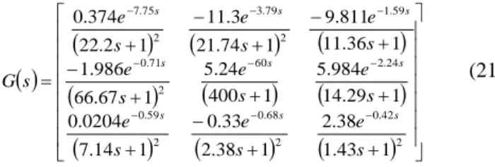
Consider the transfer function matrix of Doukas and Luyben distillation column [16]:
2 42 . 0 2 68 . 0 2 59 . 0 24 . 2 60 2 71 . 0 59 . 1 2 79 . 3 2 75 . 7 1 43 . 1 38 . 2 1 38 . 2 33 . 0 1 14 . 7 0204 . 0 1 29 . 14 984 . 5 1 400 24 . 5 1 67 . 66 986 . 1 1 36 . 11 811 . 9 1 74 . 21 3 . 11 1 2 . 22 374 . 0 s e s e s e s e s e s e s e s e s e s G s s s s s s s s s (21)For the given distillation column plant model (21) the selection of best control configuration would be carried out based on steady-state and dynamic RRA analysis (proposed approaches). Since the given distillation column model is a
3
3 control problem, therefore, the controller-dependent RRA methods would not be applicable as they are limited to
2
2 systems only.
1) The RGA analysis: a steady-state approach
The steady-state gain matrix for the distillation column model (21) can be given as:
38 . 2 33 . 0 0204 . 0 984 . 5 24 . 5 986 . 1 811 . 9 3 . 11 374 . 0
K (22)
The corresponding steady-state RGA matrix can be obtained on (4) as:
8900 . 0 1039 . 0 0060 . 0 0117 . 0 1043 . 0 0926 . 1 0983 . 0 0004 . 1 0986 . 0 (23)
As per pairing rules the pairing will correspond to those elements which are greater than '0.5' and non-negative. Therefore, the pairing based on steady-state RGA analysis for the given distillation model (21) is: 1-2/2-1/3-3.
2) The RRA analysis: a dynamic approach
The given distillation column model (21) is 33 control problem. As discussed in Section III that the controller-dependent versions of relative response array are currently limited to 22 only. Therefore, in the following section we will discuss the controller-independent versions of RRA only:
a) Controller-independent time-average RRA (CI-TA-RRA)
The CI-TA-RRA based on (10) and (11) can be obtained as: 877 . 0 101 . 0 022 . 0 014 . 0 051 . 0 037 . 1 109 . 0 950 . 0 059 . 0 TA CI (24)
The elements y1u2 , y2u1 and y3u3 of CI-TA-RRA are greater than '0.5' and close to '1'. All other elements either less than '0.5' or are negative. It is recommended to avoid the pairing of variables corresponding to the negative and less than '0.5' RGA elements. Therefore, the recommended pairing based on CI-TA-RRA analysis is '1-2/2-1/3-3'.
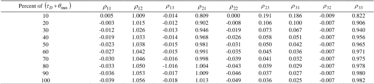
b) Controller-independent time-varying RRA (CI-TV-RRA)
Table IV shows the values of CI-TV-RRA elements based on (12) and (13) corresponding to '10' to '100' percent of the maximum time of response observation i.e. the sum of dominant time constant and maximum process dead time. It can be observed that in the whole period of response observation the elements 12, 21 and 33 remains positive and greater than '0.5' whereas all other elements remained either negative or less than '0.5' throughout. The recommended pairing based on CI-TV-RRA is: 1-2/2-1/3-3.
3) Closed-loop performance analysis
Table V shows the IMC controller settings in terms of function block parameters for Simulink model of the given plant (21).
TABLEIV:CONTROLLER-INDEPENDENT TIME-VARYING RELATIVE RESPONSE ARRAY (CI-TV-RRA) FOR DISTILLATION COLUMN PROBLEM
Percent of
D max
11 12 13 21 22 23 31 32 3310 0.005 1.009 -0.014 0.809 0.000 0.191 0.186 -0.009 0.822
20 -0.003 1.015 -0.012 0.902 -0.008 0.106 0.100 -0.007 0.906
30 -0.012 1.026 -0.013 0.946 -0.019 0.073 0.067 -0.007 0.940
40 -0.019 1.033 -0.014 0.968 -0.026 0.058 0.051 -0.007 0.956
50 -0.023 1.038 -0.015 0.981 -0.031 0.050 0.042 -0.007 0.965
60 -0.027 1.042 -0.015 0.991 -0.035 0.045 0.036 -0.007 0.971
70 -0.030 1.046 -0.016 0.998 -0.039 0.041 0.032 -0.007 0.975
80 -0.033 1.050 -1.016 1.004 -0.043 0.039 0.029 -0.007 0.978
90 -0.036 1.053 -0.017 1.009 -0.046 0.037 0.027 -0.007 0.980
100 -0.039 1.056 -0.018 1.013 -0.049 0.036 0.025 -0.007 0.982
Plant Element Desired Closed-loop Time Constantc
Controller Gain
c K
Integral Mode Gain
I c
K
Derivative Mode Gain
D c K
275 . 7
1 2 . 22
374 . 0
s
e s
7 8.0486 0.1813 97.7311
279 . 3
1 74 . 21
3 . 11
s
e s
4 -0.4936 -0.0114 -5.3654
11.36 1
811 . 9 1.59
s
e s
2 -0.4433 -0.0365 -0.3294
271 . 0
1 67 . 66
986 . 1
s
e s
7 -8.7082 -0.0653 -0.2612
400 1
24 .
5 60
s e s
50 1.0258 0.0024 28.6270
14.29 1
984 . 5 2.24
s
e s
2 0.8254 0.0536 0.8573
259 . 0
1 14 . 7
0204 . 0
s
e s
1 440.2516 30.8299 1571.6982
268 . 0
1 38 . 2
33 . 0
s e s
0.7 -8.5859 -1.8038 -10.2172
242 . 0
1 43 . 1
38 . 2
s e s
0.5 1.3062 0.4567 0.9339
Fig. 2. Comparison of output responses for the following output-input pairing: (a) 1-1/2-2/3-3 (b) 1-1/2-3/3-2 (c) 1-2/2-1/3-3 (d) 1-2/2-3/3-1 (e)
1-3/2-1/3-2 (f) 1-3/2-2/3-1.
V. CONCLUSIONS
In this paper, four new versions of the relative response array (RRA) is proposed. These versions extends the applicability of the RRA to n-dimensional systems. Both controller-independent and controller-dependent approaches are presented. The efficacy and preciseness of the proposed methods are investigated based on illustrative examples. For one of the examples the well known RGA method fails to identify the correct pairing whereas the proposed methods finds the best control configuration successfully in both the examples. The controller-dependent versions of RRA (CD-TA-RRA and CD-TV-RRA) are currently limited to 2nd and lower order processes. Their expansion to cover 3rd and higher order processes are under study.
REFERENCES
[1] S. Skogestad and I. Postlethwaite, Multivariable Feedback Control: Analysis and Design, 2 ed., New York, Wiley, 2005.
[2] M. Hovd and S. Skogestad, “Pairing criteria for decentralized control of unstable plants,” Industrial & Engineering Chemistry Research, vol. 33, pp. 2134-2139, Sept. 1994.
[3] L. Bakule, “Decentralized control: An overview,” Annual Reviews in Control, vol. 32, pp. 87-98, 2008.
(a) (b)
(c) (d)
(e) (f)
(21)
[4] P. Grosdidier, M. Morari, and B. R. Holt, “Closed-loop properties from
steady-state gain information,” Industrial & Engg. Chem Fundamentals, vol. 24, pp. 221-235, May 1985.
[5] E. H. Bristol, “On a new measure of interaction for multivariable process control,”IEEE Transactions on Automatic Control, vol. 11, pp. 133-134, 1966.
[6] P. J. Campo and M. Morari, “Achievable closed-loop properties of systems under decentralized control: Conditions involving the steady-state gain,”IEEE Transactions on Automatic Control, vol. 39, pp. 932-943, 1994.
[7] F. G. Shinskey, Process-Control Systems: Application, Design, Adjustment: McGraw-Hill, 1979.
[8] T. J. McAvoy, “Some results on dynamic interaction analysis of complex control systems,” Industrial & Engineering Chemistry Process Design and Development, vol. 22, pp. 42-49, Jan. 1983. [9] A. Jain and B. V. Babu, “A new measure of process interaction in time
domain dynamics,” in Proc. 2013 AIChE Annual Meeting, San Francisco, CA, 2013.
[10] T. J. McAvoy, “Interaction analysis: Principles and applications,” Instrument Society of América, 1983.
[11] S. Skogestad and M. Hovd, “Use of frequency-dependent RGA for control structure selection,” presented at the American Control Conference, San Diego, 1990.
[12] A. Jain and B. V. Babu, “A new measure of process interaction in time domain dynamics,” presented at the 2013 AICHE Annual Meeting, San Francisco, CA, 2013.
[13] M. F. Witcher and T. J. McAvoy, “Interacting control systems:steady state and dynamic measurement of interaction,”ISA Transactions, vol. 16, pp. 35-41, 1977.
[14] M. Morari and E. Zafiriou, Robust Process Control, Prentice Hall, 1989.
[15] M. Kinnaert, “Interaction measures and pairing of controlled and manipulated variables for multiple-input multiple-output systems: A system,”Journal A, vol. 36, pp. 15-23, 1995.
[16] P. Grosdidier and M. Morari, “Interaction measures for systems under decentralized control,”Automatica, vol. 22, pp. 309-319, 1986. [17] N. M。Naini, A. Fatehi, and A. K. Sedigh, “Input−output pairing using
effective relative energy array,”Industrial & Engineering Chemistry Research, vol. 48, pp. 7137-7144, Aug. 2009.
B. V. Babuis a vice chancellor of Galgotias University, India. He has obtained PhD from IIT Bombay. He has 29 years of teaching, research, consultancy, and administrative experience. His research interests include evolutionary compu tation, biomass gasification, fuel cells, process control and optimization, multiphase reactors etc.