Numerical studies of the interstellar medium on galactic scales

(1)

Numerical studies of the

interstellar medium on

(2)

(3)

Numerical studies of the

interstellar medium on

galactic scales

Proefschrift

ter verkrijging van

de graad van Doctor aan de Universiteit Leiden, op gezag van de Rector Magnificus Dr. D. D. Breimer,

hoogleraar in de faculteit der Wiskunde en Natuurwetenschappen en die der Geneeskunde,

volgens besluit van het College voor Promoties te verdedigen op woensdag 16 maart 2005

te klokke 16.15 uur

door

Federico Inti Pelupessy

(4)

Promotiecommissie

Promotor: Prof. dr. V. Icke Co-promotor: Dr. P. P. van der Werf

Referent: Prof. dr. L. Hernquist (Harvard University)

Overige leden: Dr. S. Portegies Zwart (Universiteit van Amsterdam) Dr. E. Tolstoy (Rijksuniversiteit Groningen)

Prof. dr. M. A. M. van de Weygaert (Rijksuniversiteit Groningen) Prof. dr. H. J. Habing

(5)

Introduction

How do galaxies work? The question may sound a bit odd, but it is the question that, in essence, galactic astronomers are trying to answer. For good reasons. The Galaxies are the most visible components of the universe. Their stars and black holes are the main sources of energy and metals after the Big Bang. Galaxies are the places where solar systems like our own form, and the dynamic and chemical evolution of our own galaxy has determined the environment from which our solar system emerged. The question how galaxies are formed and how they evolve is one of the most difficult and most interesting in astrophysics today.

Some aspects of galaxy evolution are relatively well understood. Progress on the collisionless gravitational dynamics of stars has been made in strides, and for stellar systems the distribution functions describing the population of the different possible orbits in the galaxy potential can be determined in great detail from integral field spectroscopy units (de Zeeuw et al. 2002, Cappellari et al. 2004). Also, the initial conditions of galaxy formation are becoming clear. TheΛ-cold dark matter (ΛCDM) model shows very good agreement with observations of the variations in the mi-crowave background, the large scale matter distribution and the isotopic abundances of elements formed in the Big Bang (Spergel et al. 2003). This has made theΛCDM model the standard model of cosmology. It makes precise predictions about the evo-lution of primordial density fluctuations which form the very beginnings of the galaxy formation process.

However, two unsolved problems remain in the theory of galaxy formation and evolution. The first is the nature of about 90% of the mass of galaxies as deduced from the study of rotation curves (Rubin et al. 1980) that cannot be accounted for. According to ΛCDM this unseen mass cannot be ordinary baryonic matter. Particle physicists believe that there are some good candidates among the weakly interacting sub-atomic particles that are not yet detected but expected to exist. This problem will possibly be solved in the coming years as experiments to detect these dark matter candidates are being conducted.

(8)

for the star formation process in galaxies (Elmegreen 2002). For spiral galaxies, em-pirical relations based on an instability criterion for self-gravitating disks go some way in explaining star formation (Kennicut 1989), but tests for other objects, such as dwarf galaxies, show a poor relation of this and other simple instability criteria (Hunter & Elmegreen 1998). In addition, current semi-analytic work on galaxy formation and simulations that follow the non-linear collapse of structures in the early universe fail to reproduce the observed properties of galaxies. Given the successes of theΛCDM model reproducing the large scale matter distribution and microwave background, this is thought to be due to the simplified prescriptions for the star formation and feedback processes used in these simulations. This makes sense: star formation and the associated feedback effects are complex processes that can in principle heavily modify the dynamics of the gas that is ultimately converted into stars.

The aim of this thesis is to use computer simulations to explore the star formation and feedback processes that are at work inside galaxies. All the processes related to star formation can be studied as they are taking place, because it is an ongoing process that can be studied in our own Milky Way and in nearby galaxies under a range of conditions. Therefore it is worthwhile to model current star forming systems. Our goal is then to model the structure of the interstellar medium, star formation patterns and the dynamics of the stars. Where will stars be formed in a given galaxy and how many? What is the effect of star formation on the interstellar medium and further evolution of the galaxy? To what extent does star formation trigger or inhibit further star formation? Doing this we try to match results with observed systems, which gives both insight into the evolution of these systems and constraints on theoretical model parameters.

1.1 Star forming galaxies

Star forming galaxies come in a number of forms. Our own galaxy is a large star forming spiral galaxy. It has a mass of1011_M

in stars, 1010 M in gas and a star formation rate of approximately1 M/yr. Spiral galaxies come in a variety of sizes with stellar masses of 109₋₁₀11 _M

and typical gas contents of about 10%. They form stars scattered over the disk in a characteristic spiral pattern, which can take the form of a classical ‘grand design’ spiral.

The most active star forming systems are mergers of gas rich spiral galaxies. They can show very high (>100 M/yr) rates of star formation, often obscured by dust, rendering them extremely bright in the infrared. It is thought that all Ultra Luminous Infrared Galaxies (ULIRGs) are merger events (Sanders & Mirabel 1996). These ob-jects are, with their luminosities exceeding1012 _L

among the brightest objects in the universe. At least part of current elliptical galaxies may very well be remnants from such mergers, although it remains to be seen if this formation scenario holds up against direct observation of the evolution of Ellipticals (e.g. van der Wel et al. 2004). More modest is the group of dwarf irregular (dIrr) galaxies, with masses of107₋

109_M

(9)

More-over, dIrr form stars at widely different efficiencies, varying four orders of magnitude in star formation rate per unit area (Hunter 1997). They range from blue compact dwarfs, which are characterized by a strong central star bursts to low surface bright-ness dwarfs which are almost too faint to be detected.

These dIrr galaxies form interesting model systems: the facts that they do not show spiral structure and exhibit solid body rotation means that the star formation processes in these systems take place in its most simple form, without the effects of spiral density waves or shear. In this sense these systems are ideal star formation “laboratories.” In addition their small sizes mean that we can simulate them easier at a given spatial resolution. For these reasons we will use dwarf galaxies extensively as tests and applications of our model.

In all star forming systems the same basic physical processes are at work. Star forming systems may differ in their physical properties -size, distribution of matter or chemical composition- but the basic interplay between the interstellar medium collapsing into stars and young stars injecting energy back into the surrounding gas, is the same. Thus the insights that we gain through the modelling of dIrr systems are generally applicable.

1.2 The challenge of modelling galaxies

To follow in sufficient detail the star formation processes we must be able to follow the collapse of gas due to gravitational and thermal instabilities, have a prescription for star formation, account for heating and stirring of the interstellar medium due to intense radiation, stellar winds and supernova explosions emanating from young star clusters, and to be able to follow the gas-dynamical reaction to these violent processes. We will discuss briefly the concepts behind the modelling of gravitational dynamics, the physics of ISM and the method we will use to model star formation.

The method we use for simulating galaxies is the N-body/smoothed particle hy-drodynamics (SPH) method (Hernquist & Katz 1989). Here stars and gas are rep-resented by particles. Hence, to include self-gravity, we must solve the gravitational N-body problem. In principle this is a matter of calculating all the pairwise gravita-tional forces. This is costly in terms of computing power, needingO(N2₎_operations per force evaluation (although see Makino et al. 2003 for hardware solutions to this problem). A number of approximate methods, sacrificing accuracy for speed, have been devised. We use the Barnes-Hut (BH) method (Barnes & Hut 1986).

1.2.1 The interstellar medium

(10)

Table 1.1:Overview of the phases of the ISM in the solar vicinity. Given are the densitiesn, temperaturesT, volume filling factorsfvol, mass fractionsfmass and fractionsfEof total ISM

thermal energy in the respective phases (Cox 1999).

component hni T fvol fmass fE H2 >100 10 0.001 0.5 1.5×10−3 cold HI 10−100 100 0.02 0.3 0.01

warm HI 0.1−10 8000 0.44 0.15 0.4

HII regions 10−104 ₈₀₀₀ ₀_.₀₄ ₀_.₀₁ ₀_.₀₃ Hot H+ _<₀_.₀₁ ₁₀6 ₀_.₅ ₀_.₀₀₂ ₀_.₅

the star formation process, with molecular clouds being the sites of star formation, and heating by the stars producing ionized gas.

The gas physics in our simulations is a representation mainly of the neutral gas. An important feature of the neutral interstellar medium is its two phase nature. Field (1965) considered the stability of dilute gasses and found that a two phase medium of cold and warm gas arises naturally under quiet general conditions on the cooling properties of the gas. This basic picture can be applied to the neutral phases of the ISM. It turns out that the properties of the cold and warm neutral medium could be explained in a model where they were heated by cosmic rays (Field et al. 1969). Re-cent modelling of the thermal equilibrium properties of the neutral phases by Wolfire et al. (1995, 2003) incorporating a wider range of processes, still retains this ther-mal instability. A major criticism of this picture may be that it does not account for time dependent processes. In fact, observations show large gas fractions with tem-peratures in the unstable regime (Heiles & Troland 2003, Kanekar 2003). Modern high resolution simulations of the thermal instability (Kritsuk & Norman 2002), show that a time varying UV field may induce ISM turbulence. The models we develop to calculate the non-equilibrium thermal evolution of the gas has similar equilibrium properties as the models of Wolfire et al. (1995, 2003).

1.2.2 Star formation and feedback

(11)

Apart from maintaining the hot ionized medium, supernova and stellar wind feed-back can have a profound effect on the surrounding ISM. On the one hand it stops the star formation locally, but it can enhance the star formation further out by com-pressing clouds. The collective effect of the young massive stars in an OB-association will form a hot bubble in the ISM that can sweep up material that can become unsta-ble to star formation. The question to what extent this can give rise to propagating star formation is difficult and probably this depends on local conditions. A problem for any simulation that includes supernova feedback is that a naive implementation of the energy injection as a heating term may give rise to serious errors in a cooling medium such as the ISM (Katz 1992, Fragile et al. 2003). Part of this thesis is devoted to development of a good method to account for supernova feedback.

1.3 Outline of the thesis

Chapter 2 presents the basic model of the interstellar medium that we will use to simulate galaxy sized objects. This is an extension of the model used by Gerritsen & Icke (1997) and Bottema (2003). We include for the first time realistic photo-electric heating efficiencies and we solve for the ionization, invoking cosmic rays as ionizing agent. Star formation and feedback are included, using simple but realistic prescriptions, resulting in self-regulated star formation. Different assumptions regard-ing coolregard-ing, heatregard-ing and ionization are tested usregard-ing a simple model of a star formregard-ing galaxy. The model is compared with previous models used in galactic simulations. We find that proper inclusion of stellar feedback is essential for modelling the interstellar medium.

Chapter 3 examines two new methods of implementing supernova and stellar wind feedback in N-body/SPH simulations of galaxies. The first is based upon the return of energy as random motions in the gas. The second method is based on the equations of motion of an ordinary SPH particle in the zero mass limit: we construct a separate type of particle, which we will call a pressure particle, that acts on the gas through these equations. Such a particle will be associated to each newly born stellar particle. It is checked by comparing to simple particle heating that both these methods give acceptable solutions to the Sedov blast wave test. The new methods are then tested in a dwarf galaxy model, where it is shown that they do not suffer from the problems of conventional feedback implementations. We also examine the rela-tion between HI properties and star formarela-tion, showing that our model reproduces observed correlations.

(12)

properties of dwarf galaxies. Specifically, the time-sampled distribution of the ratio between the instantaneous star formation rate and its mean is shown to match the distribution in an observed sample of dwarf galaxies.

Star forming dwarf galaxies are further examined inChapter 5, where we focus on the role of the observed structural differences between blue compact dwarfs (BCDs) and dwarf Irregular (dIrr) galaxies. Models with different gas and halo distributions are run. The resulting galaxies show a variety of star formation patterns. Galaxies with a high central gas surface density show high star formation rates, while the presence of a high central halo density will produce a central star burst. By comparing the simulations with observations it is concluded that both high central gas surface and a high central halo density are necessary for a system to exhibit BCD features.

Chapter 6 presents a method to incorporate the formation of molecular gas as part of the model. This is done by formulating a sub-grid model for molecular clouds, assumed to obey well-known scaling relations, and solving for the HI↔H2 balance set by the H2formation on dust grains and its FUV-induced photodissociation. This allows tracking of the evolution of the molecular gas seamlessly along with that of its precursor cold neutral medium HI gas. The method is applied to identify molecular regions of the interstellar medium during the evolution of a typical dwarf galaxy. We find a significant dependence of theHI→H2transition and the resulting H2gas mass on the ambient metallicity and the H2formation rate.

In Chapter 7 we show that a particle hydrodynamics method based on the De-launay triangulation field estimate (DTFE, Schaap & van de Weygaert 2000) holds special promise as an alternative to conventional SPH. The reason for this is that the DTFE density estimate is fully adaptive: the particle distribution itself generates the density field - there is no arbitrary choice kernel function or local lengthscale involved. We will show that especially in cases where the density field shows large contrasts and/or has large anisotropic features, like sheets or filaments, the DTFE es-timate is markedly superior to the kernel density eses-timate of the local density. For a hydrodynamic method based on the DTFE this will mean increased resolving power for a given number of particles. We also show that the DTFE estimate has convenient properties that will make the implementation of viscous forces better defined.

1.4 Future Prospects

The methods we have developed are suited to a wide range of problems. Two imme-diate applications are to explore the evolution of dwarf galaxies further and to model molecular gas in mergers.

(13)

parameters, and the timescales on which these processes take place will be of interest to validate cosmological and galaxy formation models.

Recent simulations (Mayer et al. 2001, Pasetto et al. 2003) have shown that a transition from dIrr to dE or dwarf Spheroidal (dSph) is plausible as a result of the repeated action of tidal fields if the dIrr orbits a large galaxy. It has not been conclu-sively determined whether a transition from dIrr to dE is to be expected in general. Various groups have put forward arguments in favour (Davies & Phillipps 1988) and against (Bothun et al. 1986, Marlowe et al. 1999) such a descendancy for the dE. Simulations testing a wider range of galactic properties and following the evolution on longer time scales may answer whether this is a viable scenario and whether we can put the various classes of small galaxies into an unified evolutionary framework. An interesting application of the H2 formation model developed in Chapter 6 would be the case of colliding galaxies. Systems like the Antennae (NGC 4038/4039), Arp 220 and NGC 6240, which are all merging systems in different stadia of their evo-lution, show large concentrations of molecular gas residing in between the nuclei of the original galaxies (e.g. Stanford et al. 1990, van der Werf et al. 1993), preceding or concurrent with the starbursts associated to these events. Hithero little work has been done in the context of numerical simulations to model the global distribution of H2gas and its relation to star formation, although a lot of work has been done on these systems using conventional N-body and N-body/SPH simulations (e.g. Toomre & Toomre 1972, Barnes 1992, Mihos & Hernquist 1994). The H2formation model is ideally suited to be applied to these kind of systems because it is fast and integrates seamlessly with these N-body simulations.

A number of improvements could be made to the code. The model should be extended to include enrichment of the interstellar medium and follow the chemody-namical evolution using metallicity dependent yields. Also, the star formation recipe may be refined further, possibly based on the identification of star forming clouds rather than on local criteria, to make it more realistic in extreme environments. Ul-timately such developments will allow us to follow the evolution of galaxies all the way from early universe to the present.

Acknowledgments.I would like to thank Natan de Vries for working with me on Chap-ter 5, Padelis Papadopoulos for co-authoring ChapChap-ter 6, and Willem Schaap for our pleasant collaboration on Chapter 7. I would also like to thank Jeroen Gerritsen and Roelof Bottema for providing software and analysis tools.

This work was sponsored by the stichting Nationale Computerfaciliteiten (Na-tional Computing Facilities Foundation) for the use of supercomputer facilities, with financial support from the Nederlandse Organisatie voor Wetenschappelijk Onderzoek (Netherlands Organisation for Scientific Research, NWO)

References

Barnes, J. & Hut, P., 1986, Nature324, 446 Barnes, J. E., 1992, ApJ393, 484

(14)

Bottema, R., 2003, MNRAS344, 358

Cappellari, M. et al., 2004, inCoevolution of Black Holes and Galaxies

Cox, A. N., 1999,Allen’s Astrophysical Quantities, Springer-Verlag, fourth edition Davies, J. I. & Phillipps, S., 1988, MNRAS233, 553

de Zeeuw, P. T. et al., 2002, MNRAS329, 513 Elmegreen, B. G., 2002, ApJ577, 206

Ferrara, A. & Tolstoy, E., 2000, MNRAS313, 291 Field, G. B., 1965, ApJ142, 531

Field, G. B., Goldsmith, D. W., & Habing, H. J., 1969, ApJ155, L149+ Fragile, P. C., Murray, S. D., Anninos, P., & Lin, D. N. C., 2003, ApJ590, 778 Gerritsen, J. P. E. & Icke, V., 1997, A&A325, 972

Heiles, C. & Troland, T. H., 2003, ApJ586, 1067 Hernquist, L. & Katz, N., 1989,ApJS70, 419 Hunter, D., 1997, PASP109, 937

Hunter, D. A., Elmegreen, B. G., & Baker, A. L., 1998,ApJ493, 595

Kanekar, N., Subrahmanyan, R., Chengalur, J. N., & Safouris, V., 2003, MNRAS346, L57

Katz, N., 1992, ApJ391, 502 Kennicutt, R. C., 1989, ApJ344, 685

Klypin, A., Kravtsov, A. V., Valenzuela, O., & Prada, F., 1999,ApJ522, 82 Kritsuk, A. G. & Norman, M. L., 2002, ApJ569, L127

Lamers, H. J. G. L. M., Panagia, N., Scuderi, S., Romaniello, M., Spaans, M., de Wit, W. J., & Kirshner, R., 2002, ApJ566, 818

Makino, J., Fukushige, T., Koga, M., & Namura, K., 2003, PASJ55, 1163 Marlowe, A. T., Meurer, G. R., & Heckman, T. M., 1999, ApJ522, 183

Mayer, L., Governato, F., Colpi, M., Moore, B., Quinn, T., Wadsley, J., Stadel, J., & Lake, G., 2001, ApJ559, 754

Mihos, J. C. & Hernquist, L., 1994, ApJ431, L9

Pasetto, S., Chiosi, C., & Carraro, G., 2003, A&A405, 931 Rubin, V. C., Thonnard, N., & Ford, W. K., 1980, ApJ238, 471 Sanders, D. B. & Mirabel, I. F., 1996, ARA&A34, 749

Schaap, W. E. & van de Weygaert, R., 2000, A&A363, L29 Spergel, D. N. et al. , 2003, ApJS148, 175

Toomre, A. & Toomre, J., 1972, ApJ178, 623

van der Wel, A., Franx, M., van Dokkum, P. G., & Rix, H.-W., 2004, ApJ601, L5 Wolfire, M. G., Hollenbach, D., McKee, C. F., Tielens, A. G. G. M., & Bakes, E. L. O.,

1995, ApJ443, 152

(15)

Chapter 2

Global models for the

interstellar medium

Abstract

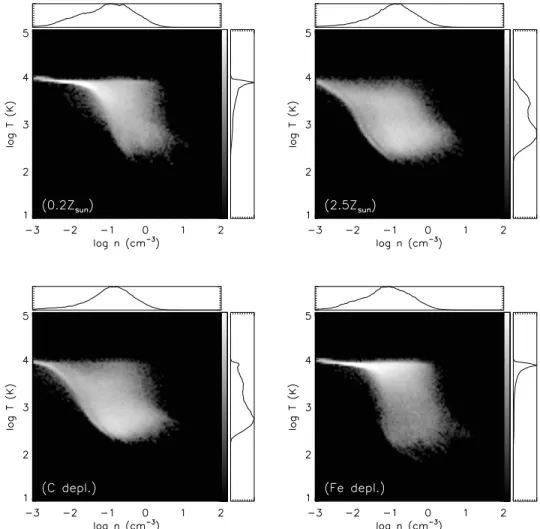
Here we present a model of the interstellar medium (ISM) for use in simulations of galaxies. The model includes the main processes important for the neutral ISM. We include for the first time realistic photo-electric heating efficiencies and we solve for the ionization, invoking cosmic rays as ionizing agent. Using an N-body/SPH model of a star forming galaxy, we test models with different assumptions regarding cooling, heating and ionization. Star formation and feedback are included using simple but realistic prescriptions, resulting in self-regulated star formation. We test the influence of metallicity and cosmic ray flux. Varying the chemical abundances, we find that C depletion gives lower star formation, while Fe depletion decreases the amount of cold gas, leaving the star formation rate relatively unaffected. We also compare with pre-vious models and show that if realistic photo-electric heating is used, stellar feedback is essential.

2.1 Introduction

(16)

attributed to a failure to account properly for physics of the ISM, especially the effects of feedback on the interstellar medium, rather than to defects of the basic properties of dark matter or the nature of gravitational forces in the model.

The state of the ISM determines where and when stars form. On the other hand, stars will seed the ISM with heavy elements and stir up the interstellar gas by putting in mechanical energy through the action of stellar winds, supernova (SN) explosions and UV radiation of young stars. From stellar evolution models the amount of met-als, and energy produced are, except maybe for extremely low metallicity stars, well known input parameters.

The complexity of the dynamics and thermodynamics of the ISM have led to a prominence of computer modelling in galactic astrophysics. However the present models for the ISM used for galactic sized objects have been rather limited in the amount of physics that is included in these models. Most models represent the ISM as a smooth fluid, where the temperature of the gas, when not taken to be isothermal, is limited to be above104_K.

In this chapter we will explore global models for the ISM in galaxies, and discuss their implementation in a smoothed particle hydrodynamics (SPH) code. The models we develop can be used to simulate a wide variety of objects and would be useful whenever star formation is important on galactic scales, such as in studies of collisions of galaxies, galaxy formation scenarios or studies of star formation in spiral galaxies or dwarf galaxies.

2.2 The N-body/SPH method

The ISM models we present below will be implemented in a derivative of the N-body/SPH code TREESPH (Hernquist & Katz 1989, Gerritsen 1997, Bottema 2003). The gravitational forces are calculated using the Barnes-Hut algorithm (Barnes & Hut 1986) and gas dynamics using SPH (Monaghan 1992). The models we present here are not limited in their applicability to N-Body/SPH codes: they can be implemented in other types of hydrodynamic codes, like Eulerian grid codes. We have opted for a first implementation into an existing N-body/SPH code, as this method is well suited for problems with open boundary conditions and arbitrary geometries, like galaxy evolution and collision problems. N-body/SPH codes are well established tools for the theoretical astrophysicists, so we will only describe both methods concisely with an emphasis on the most relevant features of the implementation used.

2.2.1 Barnes-Hut treecode

(17)

following two concepts: 1) an approximation for the gravitational force of a group of particles by cutting off the multipole expansion after the quadrupole term, and 2) the hierarchical organization of particles in an oct-tree. A force evaluation for a particle is then done by recursive opening of the nodes in the tree, conditional upon a comparison of the sizelof the node and the distancedto the centre of mass of the node:

l/d> θ (1)

where the parameterθof thecell opening criterioncontrols the accuracy of the calcu-lated gravitational forces. The BH method has been widely used in numerical N-body simulations, due to itsO(N log N)scaling and its ability to be applied efficiently to general mass distributions. In astrophysics the method has found wide application in, for example, cosmological simulations, galaxy collision and star formation simu-lations. It has been shown that it is generally acceptable to use BH for collisionless N-body dynamics (Barnes & Hut 1989). However the classical BH opening criterion (1) can fail in exceptional circumstances (Salmon & Warren 1994). Also it was shown by Springel et al. (2001) that it will give large fractional force errors if particles are subjected to large cancelling forces such as those experienced in the smooth matter distributions found in the early universe. A similar problem may also occur for galaxy simulations, especially in the central regions of galaxies where particles experience large cancelling forces from the rest of the galaxy. Springel et al. (2001) propose an alternative opening criterion,

Ml4> α|a|d6 (2)

whereMis the total mass contained in the node,ais an estimate of the acceleration,

in practice this is the acceleration of the previous time step, and α the parameter controlling the accuracy of the force calculation. We have compared the accuracy of the BH criterion and the Springel criterion and found that the latter indeed gives smaller fractional force errors in the central regions of the galaxy.

2.2.2 Smoothed Particle Hydrodynamics

Smoothed Particle Hydrodynamics (Gingold & Monaghan 1977, Lucy 1977) is a par-ticle based method for gas dynamics. It is based on an estimate of the local density of a continuous fluid respresented by a finite set of particles using a kernel function

W(r,h). Thus, for a set of particles with massesmiand smoothing lengthshiwe have

ρi =

X

j

mjW(|ri−rj|,hi) (3)

for the densityρi at particle positionsri. The kernel functionWis usually (and also here) taken to be the spline kernel of Monaghan & Lattanzio 1985:

W(r,h) = 1

πh3







1−3 2 r h 2 +3 4 r h

0≤r≤h

1 4(2−

r h)

3 _h_≤_r_≤_2h

0 otherwise

(18)

dynamics, but this is done more elegantly starting from the discretized Lagrangian for a compressible non dissipative flow, with adiabatic indexγ(Rasio 1999),

L = N X i=1 mi 1 2v 2 i + 1

γ−1Aiρ

γ−1 i

, (4)

where mi is the mass of particle i (1 ≤ i ≤ N), vi its velocity, Ai is the entropic function, defined by (Pi being the pressure): Pi = Aiργi. We will formulate the dynamic evolution of the internal energy in terms of this entropic function. The internal energyuiitself is obtained through

ui =

Ai

γ−1ρ

γ₋1

i (5)

Treating the flow adiabatic for the moment and assuming constant smoothing lengths

hi, it is easy to recover the SPH formalism from the Lagrangian equations of motion for(q,p) = (r1, ..rN,v1, ..,vN). Notice that the procedure we have outlined here is not specific for the kernel based density estimate of Eq. (3), indeed in Chapter 7 we will present an alternative method for gas dynamics by using the Delaunay Triangulation Field Estimator for the density, which is a much better density estimate in regions of high density contrasts or anisotropy. The dynamic range of conventional SPH is im-proved by the use of adaptive smoothing lengths. Normally this is done by choosing thehi such that the number of neighbours within a smoothing lengthhi is (more or less) constant for every particle. This introduces errors in energy and/or entropy con-servation (Hernquist 1993, Nelson & Papaloizou 1993). This is because the variability ofhi introduces extra∇hcorrection terms into the dynamical equations, inclusion of which is, although possible (see Nelson & Papaloizou 1994), cumbersome. An al-ternative approach is to consider hi as dynamic variables in the Lagrangian (4) and introduce constraints which will determine these extra variables (Springel & Hern-quist 2002). Taking as the set of constraints

φ= 4π 3 h

3

i(ρi+ ˜ρ)−Mr= 0 (6) which (for constant density) is simply the requirement that the mass enclosed within a smoothing length is fixed. In this equationMr= ¯mNnbwith mean particle massm¯ and a target number of neighboursNnb. Comparing with Springel and Hernquist (2002) we add a termρ˜to limit the smoothing lengthhi. Without this term the smoothing length grows ashi → ∞whenρi →0, leading to a very high number of neighbours for particles on the edge of the simulation. A maximum h3

i,max = 3Mr/4πρ˜leads to a minimumρi,min = mi/πh3i,max = 4˜ρ/3Nnb, which, to ensure errors due to poor sampling for particles withρi .ρ˜, are limited, is set to be lower than the intergalactic medium density by a suitable choice ofρ˜.

(19)

this yields the following system of dynamic equations we solve in the code, including artificial viscosity terms (Wij(hi) = W(|ri−rj|,hi)):

dvi

dt =−

N X j=1 mj ( fi Pi ρ2 i

∇iWij(hi) + fj

Pj

ρ2 j

∇iWij(hj) + Πij∇W¯ij

)

(7)

with thefidefined by:

fi=

1 + hi 3(ρi+ ˜ρ)

∂ρi

∂hi

−1

(8)

The artificial viscosity Πij is necessary to smooth out discontinuities to resolvable scales, and we can take any one of the standard forms (Monaghan 1992, Hernquist & Katz 1989). Here,W¯ij = Wij(hi) + Wij(hj)is a symmetrized form of the kernel. The thermodynamic state of the gas is determined by integrating the entropic function according to

dAi

dt =−

γ−1

ργi

(Γ−Λ) + 1 2

γ−1

ργi−1 N

X

j=1

mjΠijvij· ∇iW¯ij (9)

HereΓandΛrepresent the external heating and cooling terms, which will be derived from a consideration of the physical processes that we want to include to model the ISM.

2.2.3 Some notes on implementation

The code we use is written in FORTRAN 90, and parallelised for use on shared mem-ory architectures using OpenMP compiler directives.

We must solve Eq. (6) for the smoothing lengthshi. This can be done efficiently using Newton-Raphson iteration, seconded by recursive bisection.

2.3 Physical processes of the ISM

Our model for the ISM will be mainly geared towards the representation of the neutral atomic phases of the ISM. Roughly speaking we will follow the ISM of our model galaxies as long as the temperature is higher than 100 K and densities are greater than100cm−3_{. We will consider the formation and subsequent evolution of molecular} clouds to be part of the process of star formation. The process of star formation in these clouds is not explicitly present in our model, but implicitly in the recipe for star formation (section 2.5.1).

A comprehensive model for the warm and cold neutral medium (WNM, CNM) that is similar to our model, albeit more extensive, was formulated by Wolfire et al. (1995, 2003). They explored the thermal equilibrium of the neutral ISM, in the context of a static model of the Milky Way. They concluded that their model was consistent with a number of observations, amongst which dust emission and [CII] line observations.

(20)

0.0001 0.001 0.01 0.1 1 xe

0.2 0.4 0.6 0.8 1

Φ

H

20 35 50

Figure 2.1:Secondary ionization functionφH

for different electron energies. Curves are la-belled with the corresponding energy of the secondary electron (in eV).

realistic cooling by a variety of atomic species. This improves on the treatment of previous models used in galactic simulations by not assuming a priori the ionization and by taking into account the efficiency decrease of photoelectric heating by grain charging. Also our cooling curves are more accurate and composed for arbitrary abun-dances, which allows us to explore the effect of variations of composition on the ISM.

2.3.1 Ionization

Even neutral interstellar gas retains some ionization. Gerritsen & Icke (1997) found that the results of their model depended on the ionization fraction xe ≡ ne/nH as-sumed for temperatures belowT≈14000. For example forxe= 0.1they found a star formation rate 4 times higher than forxe = 0.01while the amount of cold gas was roughly ten times lower for the lowxe case. The reason for this is that the cooling power is proportional toxe. At low temperatures cooling is mainly due, if molecu-lar gas is absent, to excitation of fine structure levels of neutral and ionized species. The excitation efficiency for collisions by electrons is much higher than that of neu-tral hydrogen, so for quite low ionization levels (xe > 0.001) the electron fraction will determine the amount of cooling. Gerritsen & Icke (1997) did not solve for the ionization, so they had to assume a value and for their standard model they settled forxe = 0.1. This seems to be reasonable for the solar neighbourhood (Cox 1990), however one would expect it to vary with local temperature and density, hence it is necessary to solve for ionization.

(21)

regions. We will lump the effect of HII regions together with the effects of stellar winds and supernovae as the mechanical luminosity of young stellar clusters. Pho-tons with energies below 13.6 eV will propagate freely through the ISM, and any elements with ionization potentials less than 13.6 eV will be assumed to be at least singly ionized. Of the elements we include in our model these are C, Fe and Si. In practice the minimum ionization fraction in the simulation will be determined by the abundance of carbon, as it is the most abundant. Ionization of these species is also important for the cooling, in the next section we will see that C+_{, Si}+ _{and Fe}+ _are important coolants.

The main source of ionization in the neutral medium is probably collisions with cosmic rays. To calculate the resulting electron fractionxe, we solve for the ionization equilibrium of H and He only,

αicollneni+ξCRni =αi+1re neni+ (10)

with the ni as the densities of i =H, He, He+ and He++, αicoll = αicoll(T) and

αi

re = αire(T) the appropriate collisional ionization and recombination rates. For these we take the fits of Voronov (1997)1_{. Here,}_ξ

CRis the total cosmic ray ionization rate, which is determined by the primary ionization rateζCRmultiplied by a factor ac-counting for the secondary ionizations by the energetic electrons produced in primary ionization events (Wolfire et al. 1995),

ξCR=ζCR 1 +φH(E,xe) +φHe(E,xe). (11) The functionsφH_(E_,_x

e)andφHe(E,xe)give the number of secondary ionizations of hydrogen and helium per primary ionization. These depend on the energyEof the secondary electron (we take a typical value of 35 eV) and the electron fractionxe. We use the analytic fits forφHandφHeprovided in the appendix of Wolfire et al. (1995). Qualitatively, the number of secondary electrons increases withE, as expected, while for increasingxe, it decreases (the secondary electron will loose its energy more easily through Coulomb interactions for high ionization fractions). For the primary ioniza-tion rate we take a standard value of

ζCR = 1.8×10−17s−1. (12)

Note that the primary cosmic ray ionization rateζCR is mainly due to particles with energies below 100 MeV, which are shielded from direct observation by the helio-sphere (extrapolation from Pioneer and Voyager data yields a rate ofζCR= 3×10−17, Webber 1998) and also expected to vary substantially due to their low travelling lengths. Presumably their production sites are regions of star formation, and calcula-tion of the propagacalcula-tion of these cosmic rays is complicated. The canonical value (12) comes from chemical modelling of molecular clouds (Van Dishoeck & Black 1986) and may not be appropriate for the diffuse ISM (McCall et al. 2003). So the actual value of the cosmic ray flux that is appropriate is uncertain (however this does not mean that details as (11) are superfluous, because it introduces a feedback ofxe on the ionization rate that is present regardless of the actual value forζCR).

The system of Equations (10) is easily solved by iterating overxe, in practice we also tabulate its solutions for quick referencing by interpolation in temperature T

(22)

1 2 3 4 5 6 7 8 log THKL

-3

-2

-1 0 1

log

xe

Ζn=1.8´103

Ζn=1.8´10-2

Figure 2.2:Ionization fraction xe = ne/n for different values of ζCR/n, increasing from

ζCR/n = 1.8×10−2toζCR/n = 1.8×103in factors of 10.

and ζCR/n. In Fig. 2.2 we have plotted the resulting ionization fraction for solar metallicities.

We solve for the ionization to get an estimate of xe. Metals will not contribute significantly and hence we do not solve for their ionization. The abundance of the different ionized species needed for the cooling rates (see below) will be assumed to be in CIE. For calculation of CIE a more complete set of processes including charge exchange is considered (included in theDoricpackage, Raga et al. 1997, Mellema & Lundqvist 2002).

Apart from cosmic ray ionization a seizable contribution is expected from X-ray ionizations. We will not consider these separately, because of the above mentioned uncertainties in the cosmic ray ionization rate, and because the physical process of X-ray ionization is similar to cosmic ray ionization.

2.3.2 Cooling processes

A heated, partially ionized gas cools through the conversion of kinetic energy into luminosity by collision processes, and the efficiency of cooling is a sensitive function of the composition of the gas. The cooling in the low density limit can be approximated by

Λ = n2Λ?(T) (13) For the cooling curve Λ?_(T) _{a number of pre-compiled cooling curves for specific}

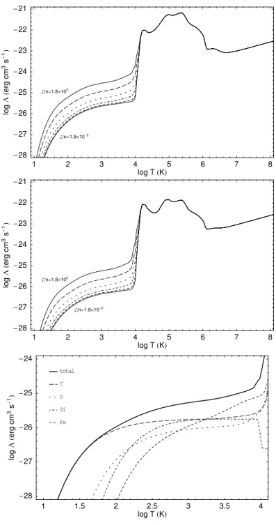
metallicities exist (e.g. Dalgarno & McCray 1972, Sutherland & Dopita 1993). We cal-culate the cooling curve for general abundances using recent atomic data. In Fig. 2.3 we have plotted the cooling curve

Λ?(T) =X

i,j

Xij

xeLeXij(T) + L

H Xij(T)

(14)

for solar and0.2×solar metallicity. The functionsLe

XijandL

H

Xijgive the cooling power

(23)

1 2 3 4 5 6 7 8 log THKL

-28 -27 -26 -25 -24 -23 -22 -21 log L H erg cm 3s -1L

Ζn=1.8´103

Ζn=1.8´10-2

1 2 3 4 5 6 7 8

log THKL

-28 -27 -26 -25 -24 -23 -22 -21 log L H erg cm 3s -1L

Ζn=1.8´103

Ζn=1.8´10-2

1 1.5 2 2.5 3 3.5 4

log THKL

-28 -27 -26 -25 -24 log L H erg cm 3s -1L Fe Si O C total

Figure 2.3:Cooling curves. Top panel: Cooling curves forZ = Z_{, labelled with values of}

ζ/nas in Fig. 2.2. Centre panel: Cooling curves for Z = 0.2×Z, idem. Bottom panel:

(24)

10 100 1000 10000 100000. G0T.5ne

0.002 0.005 0.01 0.02 0.05 0.1

Εuv

T=102_K

103 10

4

Figure 2.4:Full UV heating efficiencyUV.

with a relative abundanceXij. We takeLe

Xij from a recent compilation of atomic data

from theDoric package (Raga et al. 1997, Mellema & Lundqvist 2002 ), while we calculateLH

Xij, using thePopratioprogram (Silva & Viegas 2001). Also in Fig 2.3 we

have plotted the contributions of the various elements to the cooling for the most important coolants. For solar metallicity carbon (in the form of CII) is the main coolant at low temperatures (T<1000K). Iron is dominant at temperatures between

3000and10000K. Si can also be a substantial coolant at intermediate temperatures (around1000K).

Note that apart from the dependency on the composition of the gas, cooling is strongly dependent on the ionization fraction, becauseLe

Xij is typically a factor1000

bigger thanLH Xij.

2.3.3 Heating processes

The most important heating mechanism in the neutral ISM is photoelectric heating from small grains and PAHs (Watson 1972): UV radiation will heat gas in the presence of dust through the ejection of electrons from these particles. We will use the results of modelling by Bakes & Tielens (1994) to calculate this heating. The heating for a radiation fieldG0, normalised to Habing’s (1.6×10−3_{erg cm}−2_s−1_{, 1968), is given} by

Γ = 10−24

UVn (Z/Z) G0 erg cm−3s−1, (15) where the heating efficiencyUVis fitted by

UV= 4.9×10 −2

1 + [ξgr/1925]0.73

+3.7×10

−2 _T_/₁₀40.7

1 + [ξgr/5000]

(16)

(25)

0.0001 0.001 0.01 0.1 1 xe

0.2 0.4 0.6 0.8 1

Eh

H

normalized

L

20 35

50

Figure 2.5:Cosmic ray heating functionEh. Plot of the fraction of the secondary electron

energy used for heating. Curves are labelled with secondary electron energy.

electrons need to overcome an extra potential barrier to get expelled from the grains. This lowers the energy available for heating the gas, which decreases the efficiency for increasingξgr(Fig. 2.4). This has important implications for the heating rates in our model, effectively reducing the strength of the radiative feedback for high radiation fields to_∝G0.27

0 . So compared to Gerritsen & Icke (1997) and Bottema (2003), who took a constant efficiency, the UV radiation feedback will be less important for estab-lishing star formation equilibrium. Note also that in this case the heating becomes a strong function of ionization, as high ionization reduces grain charging.

The heating of Eq. (15) scales with metallicity (assuming the dust-to-gas ratio scales with Z), UV field, density and takes into account grain charging. We do not take into account the finer points of dust physics, notably the dependence of the heat-ing on the shape of the spectral energy distribution of the impheat-ingheat-ing radiation field and the dependence of the heating on size and shape distribution of the dust grains. Both effects can change the heating rate by 25%, when varying the parameters under reasonable constraints (Wolfire 1995). In principle the distribution of the grain sizes, shapes etc could come out of a model for the formation, processing and destruction of dust grains and PAHs, but clearly this is a very complicated problem. We will just assume the same grain distribution to be present everywhere.

The UV field needed in Eq. (15) is calculated from the distribution of stars, anal-ogous to the way the gravitational forces are calculated. Dust extinction is not taken into account explicitly, although we do roughly model the extinction of UV light from young stellar clusters by the remnants of the natal clouds by increasing the emission of UV light from 25% to 100% of the nominal luminosity over a period of 4 Myr.

Normally photoelectric heating dominates over X-ray and cosmic ray heating, but this is not the case in the outer parts of galaxies where both density and radiation field drop. In these regions we will provide for heating by including cosmic ray heating, which for a primary ionization rateζCRis given by

(26)

The functionEh(E,xe)gives the heat deposited for every primary electron of energyE (of typically 35 eV), given in Wolfire (1995). We have plotted this function in Fig. 2.5. In principle X-ray heating may also be important, but as its effect and magnitude is similar to that of cosmic ray heating (and this term is subject to some uncertainty, see discussion in section 2.3.1), we do not include it separately.

2.3.4 Molecular gas

We will not consider the formation of molecular gas in this chapter. However in view of the importance of molecular gas, both as fuel for the formation of stars, and as a diagnostic tool in extra-galactic studies of star formation, we will here give an overview of the relation of molecular gas and the gaseous phase of our simulation. In Chapter 6 we will investigate the formation of the most important molecule, H2, in some detail.

A direct implementation of H2 formation from first principles in current galaxy scaled computer simulations is, both from the viewpoint of the necessary resolution as from the viewpoint of necessary physics, impractical. In our simulation the physics of molecular cloud formation is considered to be part of the star formation process, captured in a basic but plausible model (see below). A result of this approach is that the star formation rates will not be set by molecular cloud physics, but at a larger scale: by the surface density of the gas, cooling properties of the neutral medium and large scale instabilities. This is consistent with the prevailing view of star forma-tion (Elmegreen 2002). The mass that is contained in the molecular phase will be present in the cold phase in our simulation, and thus, while assessing the amount of cold gas resulting from our simulations, one must keep in mind that this includes a considerable amount of what would be molecular gas.

Note that diffuse H2gas is also absent in our model. This may be a more serious omission. Diffuse H2 may be present at abundances of10−3₋₁₀−4 _{in the neutral} medium (Richter et al. 2001) and at this level it could affect the cooling of the neutral medium substantially, as the cooling efficiency of H2gas is about a factor103 higher than for our neutral gas (Le Bourlot et al. 1999).

2.4 Equilibrium models

The different heating and cooling processes we have discussed in section 2.3 consti-tute a reasonably complex model for the ISM. It is certainly more realistic than most previous models that have been used in galaxy simulations, as it attempts to include the cold and warm phases of the neutral ISM. To get an idea of the properties of the resulting ISM it is instructive to explore the thermal equilibrium state of our model and compare it to the previous models of Gerritsen & Icke (1997), Bottema (2003) and also to the equilibrium models of Wolfire et al. (1995).

(27)

of processes in the ISM that are acting on timescales comparable to the timescales associated with the thermal evolution of the gas.

A region of cold gas subjected to an increase in UV radiation will quickly heat to a temperature ofTeq= 104K in a time

theat=

ρueq

Γ =

3/2kTeq

Γ ≈ 106

(Z/Z) G0

yr (18)

The time a region of density ρ and internal energy u = 3/2kT needs to return to equilibrium after a significant perturbation is given by the cooling time,

tcool=

ρu Λ =

3/2kT fHnΛ?

(19)

which gives roughly tcool ≈ 105 yr (n = 10 cm−3, T = 100 K) for the CNM and

tcool≈107yr (n = 0.1cm−3,T = 104K) for the WNM.

Variations in the local UV field were studied by Parravano et al. 2003. They found variations on timescales of107−8_{yr. This is comparable to timescales in the WNM but} much slower than the timescales of the CNM. A similar conclusion holds for supernova perturbations. Wolfire et al. (2003) estimated for the characteristic time of these that

tshock= 5.3×106yr.

So we see that under quiescent (solar neighbourhood) conditions thermal equi-librium is a reasonable assumption for the CNM and marginally good for the WNM, whereas for more active regions this assumption will become increasingly question-able, especially for the WNM but also for the CNM, since the frequency of most of the perturbing agents scales with star formation rate. A large fraction of out-of-equilibrium gas is consistent with recent HI absorption line studies, which find that a substantial fraction (around 50%) of the WNM is in an unstable temperature range, and thus presumably not in equilibrium (Heiles & Troland 2003, Kanekar 2003).

2.4.1 Heating and ionization assumptions

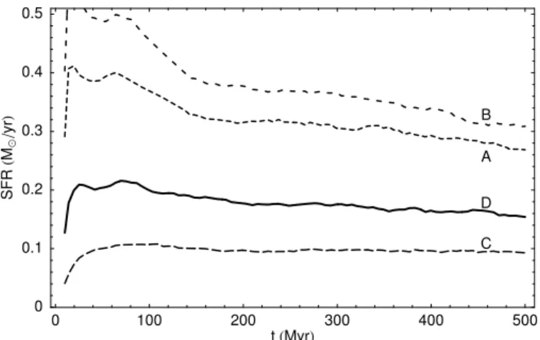
To explore the effect of the different heating and ionization processes that are new to our ISM model and to compare these to previous work, we explore a number of different models, designated A B C and D, of increasing complexity. For the mo-ment we consider solar metallicity. The first of these models (model A) is the same, except for the cooling, as the model used in Gerritsen & Icke (1997): a constant heating efficiency (UV= 0.05) and a constant ionization fraction (xe = 0.1). Model B has the heating efficiency of Eq. (16), while retaining constant ionization. Model C has constant heating efficiency while solving for ionization and finally model D is our complete model solving for the ionization and using the full heating efficiency. Fig. 2.6 shows for these four models the equilibria of pressure, temperature, electron fraction and heating (=cooling) rate.

(28)

-2 -1 0 1 2 3 log nHcm-3_L

0 1 2 3 4 log L H 10 -27 erg s -1L

-2 -1 0 1 2 3

log nHcm-3_L

-4 -3 -2 -1 0 log xe

-2 -1 0 1 2 3

log nHcm-3_L

1 2 3 4 5 6 log P H K cm -3L

-2 -1 0 1 2 3

log nHcm-3_L

1 1.5 2 2.5 3 3.5 4 4.5 log T H K L D C B A

Figure 2.6:Thermal equilibrium properties of models A,B,C and D. Shown are (in order: top left, top right, bottom left and bottom right) the pressure, temperature, cooling rate and ion-ization fraction in thermal equilibrium as a function of density. In the plot results are shown forZ = ZandG0= 10.

see that the models which do not solve for the ionization (A and B) seriously over-estimate the ionization at high densities and thus overover-estimate the cooling resulting in lower temperatures. The models which do not use the full heating efficiency (A and C) overestimate the heating, especially at low densities, hence these have higher temperatures at low density. The total effect is that the range of pressures for which the ISM is unstable will be much greater in the simpler models.

If we compare Fig. 2.6 to Fig. 3 of Wolfire et al. (1995) we see that our model D is very similar, showing very similar trends for electron fraction and heating rate. Hence our model captures most of the essential physics of the Wolfire et al. model.

In a complete simulation the conditions of UV and supernova heating will vary from place to place. This will change the relations of Fig. 2.6. So next we will explore the effect of variation of UV and cosmic ray heating.

2.4.2 UV field and Cosmic rays

(29)

-2 -1 0 1 2 3 log nHcm-3_L

0 1 2 3 4 log L H 10 -27 erg s -1L

-2 -1 0 1 2 3

log nHcm-3_L

-4 -3 -2 -1 0 log xe

-2 -1 0 1 2 3

log nHcm-3_L

1 2 3 4 5 6 log P H K cm -3L

-2 -1 0 1 2 3

log nHcm-3_L

1 1.5 2 2.5 3 3.5 4 4.5 log T H K

L G0=1

G0=10

G0=102

Figure 2.7: Thermal equilibrium properties of model D: varying UV heating.Z = Z.

gas will ’move up’ quickly to a newG0curve , cf. (18).

An increase in cosmic ray flux shows a similar pattern: In Fig. 2.8 we have plotted the pressure-density relation for different cosmic ray fluxes. A high value for the cosmic ray ionization rate may very well be appropriate: for diffuse clouds in the solar neighbourhood McCall et al. (2003) found that a value of the cosmic ray ionization rate of up toζCR= 1.2×10−15was necessary to account for the observed abundance of H+

3.

2.4.3 Varying chemical composition

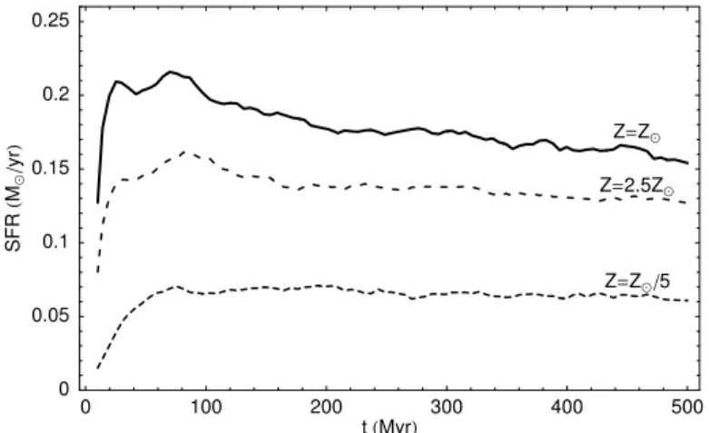
In Fig. 2.9 we show the effect of varying the chemical composition. A lower metal-licity shifts the unstable region to higher density and pressure, while also extending the range of unstable pressures. Note that the ISM model is still relatively insensitive to variations in metallicity. This is because we scale the dust-to-gas ratio, and thus the heating efficiency, with metallicity. Both cooling and heating are to first order proportional to metallicity. In Fig. 2.10 we show theZ = Z/5model in more detail. Pressure, temperature and electron fraction are similar to the model for solar metal-licity, although the cooling rate shifts down. The cooling and heating times (19) and (18) scale inversely with metallicity. So while varying the metallicity has relatively little effect on the equilibrium state, it will affect our full dynamical modelling.

(30)

-2 -1 0 1 2 3 log nHcm-3_L

1 2 3 4 5 6

log

P

H

K

cm

-3L ΖCR=7.2´10-16 ΖCR=1.8´10-16 ΖCR=9´10-17 ΖCR=1.8´10-17

Figure 2.8:Equilibrium pressure-density relation for different cosmic ray fluxes,G0= 10.

-2 -1 0 1 2 3

log nHcm-3_L

1 2 3 4 5 6

log

P

H

K

cm

-3L _{Fe,Si depleted}C depleted

Z=Z50 Z=Z5 Z=Z Z=2.5 Z

Figure 2.9:Equilibrium pressure-density relation for different chemical compositions,G0 = 1.

2.5 Star formation and its effects

From the point of view of our simulation star formation is micro physics that is not resolved. The formation of stars in dense clouds of the interstellar medium is a com-plex process that is still very much an active field of research, and there is no general theory to predict the star formation rate of a given region of the ISM. However from observations and theory some key processes are identified. Probably the most influ-ential observational relation is theSchmidt law(Schmidt 1959): the empirical finding that the star formation rate (SFR) of disk galaxies varies with gas surface densityσg asSFR ∝σ1.5

(31)

-2 -1 0 1 2 3 log nHcm-3_L

0 1 2 3 4 log L H 10 -27 erg s -1L

-2 -1 0 1 2 3

log nHcm-3_L

-4 -3 -2 -1 0 log xe

-2 -1 0 1 2 3

log nHcm-3_L

1 2 3 4 5 6 log P H K cm -3L

-2 -1 0 1 2 3

log nHcm-3_L

1 1.5 2 2.5 3 3.5 4 4.5 log T H K

L G0=1

G0=10

G0=102

Figure 2.10:Thermal equilibrium properties of model D withZ = Z/5, varyingG0

2.5.1 Star Formation

We use the star formation recipe of Gerritsen & Icke (1997). A region is considered unstable to star formation if the local Jeans massMJ,

MJ= πρ

6

πs2

Gρ

3/2

(20)

withsthe sound speed, is smaller than the mass of a typical molecular cloudMref,

MJ<Mref. (21) The rate of star formation is set to scale with the local free fall time,

τsf = fsftff = √fsf

4πGρ. (22)

The delay factorfsf accounts for the fact that collapse of molecular clouds is inhibited by either turbulence or magnetic fields (Mac Low & Klessen 2004, Shu et al. 1987). Its value is uncertain, but from observations a valuefsf ≈10seems reasonable (Zuck-erman & Palmer 1974).

There are many different ways to let stars form locally on the timescale given by Eq. (22). One way to achieve this, followed by Gerritsen & Icke (1997) is to wait for a timeτsf and then proceed to form stars. Another is just to assign a probability1−

(32)

differences between the two methods: in the stochastic case star formation may also be delayed beyondτsf, and where this is the case the unstable region may collapse to higher densities than it would in the fixed delay case. The fixed delay case, on the other hand tends to synchronize star formation over regions that become unstable at the same time, which leads to a sudden onset of star formation, for example in the beginning of the simulation. We will note whenever a choice of either one has a substantial impact on the results.

Once a gas particle is determined to be forming stars, a fractionsf of the mass is converted to stars. This sets a minimum to the star formation efficiency (a neighbour-hood of gas particles of about 64 particles that has become capable of star formation will thus form at least a fractionsf/64of stars). The actual efficiency of star forma-tion is determined by the number of stars needed to quench star formaforma-tion locally by the UV and SN heating and is determined by the cooling properties of the gas and the energy input from the stars.

Thus the local star formation rate will be given by

dρ?

dt =− dρgas

dt =

sf

τsf

ρJU (23)

whereρJUindicates the ’Jeans unstable’ gas, satisfying (21). The effective timescale for star formation isτeff = τsf/sf = fsftff/sf, so different combinations of fsf and

sf will give the same star formation rate. In case of a fixed delay time (Gerritsen & Icke method), it is appropriate to take a constant mass fractionsf for the newly formed star particles, while in the stochastic method we can form star particles of fixed mass, and thus biggersf as gas particles become lighter, as long as we increase

fsf accordingly.

The recipe is certainly not unique, we have based our choice on the following considerations: it is simple and based on presence of substructure and the driving role of gas self gravity, and it reproduces the Schmidt law without actually imposing it (Gerritsen & Icke 1997). It does assume substructure to be present (actually its assumption is more restrictive still, namely that substructure is mainly atMref sized clouds, but this is not overly important). For this type of simulation one is always restricted by the limited ability to follow the star formation process, so we are forced to adopt a phenomenological description at some level.

Another concern that could be addressed is that the SF according to this recipe is independent of metallicity, other than that induced by the metallicity dependence of the cooling. If cloud collapse is regulated by magnetic fields (Shu et al. 1987), a more detailed dependence of the delay factor fsf on for example ionization may be appropriate.

We assume the stellar initial mass function (IMF) to be universal. We take a Salpeter IMF with a lower mass cutoff of0.1 Mand an upper mass cutoff of100 M. The shape of the IMF determines the amount of heavy stars, and thus the amount of UV and supernova feedback. If the IMF would vary according to local conditions this will have its effect on star formation. Observations are consistent with a universal IMF over a wide range of ISM conditions, however there are some hints that for high radiation fields and/or low metallicities relatively more high mass stars are formed (e.g. Lamers et al. 2002).

(33)

prevents the simulation from violating the resolution requirements for self gravitating SPH of Bate & Burkert (1997) and Whitworth (1998). For SPH the local Jeans mass should be bigger than the local mass resolution,

MJ>NmSPH, (24) otherwise artificial clumping or inhibition of clumping may occur. This condition is just Eq. (21), ifMref is chosen equal to the local mass resolution, Mref = NmSPH (N is the number of SPH neighbours, and mSPH the mass of SPH particles). We will do so, and our simulation will thus follow collapse and fragmentation of the ISM from the WNM to the CNM, but at a certain point (Eq. 21) the simulation can no longer reliably follow this process. At this point further assumptions regarding the details of star formation enter through Eq. (22). In practice this limit lies at a very physically relevant region of parameter space, namely at temperatures and densities where molecular clouds should form in the CNM. So our simulation tracks the evolution of the WNM and CNM up to a point where a phase of the ISM forms that can be trusted to form stars, at efficiencies that are somewhat constrained by observations. As we increase resolution and decreasemSPH we can decrease Mref and follow the collapse further.

2.5.2 Stellar model

We calculate the FUV luminosities of the stellar particles from the age and metallicity of the stars and Bruzual & Charlot (1993, and updated) population synthesis models. For this the integrated flux between912 and 2100A is calculated from single burst˚ models with a salpeter IMF with a low mass cutoff of0.1 Mand high mass cutoff of

100 M. It is not entirely clear if interpolation in metallicity from the coarse grid data available is the best strategy, so in case we run a model with a metallicity different from the Bruzual & Charlot models we just take the synthesis model with the closest matching metallicity. We roughly account for the extinction of UV light of young stars by their natal cloud by increasing the flux from 25% at birth to 100% at 4 Myr, in accordance with counts of UV sources in the neighbourhood of star forming clouds (Parravano et al. 2003, and references therein).

2.5.3 Feedback

(34)

5 6 7 8 9 log tHyrL

30 31 32 33 34 35

log

Lmech

H

erg

s

-1M

-1L

adopted SN winds total

Figure 2.11:Mechanical energy output from stellar cluster. Plotted as a function of age of a single burst of star formation atZ = Zare the separate contributions from stellar winds (short dashed) and supernovae (long dashed), as well as the total mechanical luminosity(drawn) from Leitherer et al. (1999). The dotted line indicates the mechanical luminosity of the stellar particles adopted in our simulation.

While the mechanical energy output of stars can thus be estimated with reasonable accuracy, it has proven to be difficult to include the effects of feedback completely self-consistently in galaxy sized simulations of the ISM. The reason for this is that the effective energy of feedback depends sensitively on the energy radiated away in thin shells around the bubbles created. This will mean that the effect of feedback is not reliable unless prohibitively high resolution is used. In SPH codes there have been conventionally two ways to account for mechanical feedback: by changing the thermal energy input and by acting on particle velocities. Both are unsatisfactory, as the thermal method suffers from over cooling (Katz 1992) and the kinetic method seems to be too efficient in disturbing the ISM (Navarro & White 1993). Here we use a new method based on the creation at the site of young stellar clusters ofpressure particlesthat act as normal SPH particles in the limit that the mass of the particle

m→0, for constant energy (see Chapter 3 for more details). For the energy injection rate we take ˙E =snnsnEsn/∆t, with supernova energyEsn = 1051erg, an efficiency parameter sn = 0.1, number of supernova nsn per solar mass of stars formed of

nsn = 0.009 and an active period∆t = 3×107 yr (approximately the lifetime of a

(35)

2.6 Putting it all together

The combination of hydrodynamics, self-gravity and the ISM models of section 2.4 with our star formation and feedback recipes will set up a self regulated ISM. The distribution of temperature, density, etc. of the gas and amount and location of star formation will be the outcome of the interaction between the competing processes of heating and cooling, feedback and collapse. We will test this global model for the ISM of star forming galaxies by applying it in a simulation of a suitable galaxy.

2.6.1 Initial conditions

For our purposes we need a simple model galaxy. We construct a three component model of a typical star forming disk galaxy with a gaseous disk, a stellar disk and a dark halo.

The stellar disk has a mass of 1010 _M

and is constructed to be approximately exponential,

ρdisk(R,z) = Σ0

2hz

exp(−R/Rd)sech2(z/hz), (25)

for a central surface density Σ0 = 5×108 M/kpc2, disk scaleRd = 1.8 kpc and a vertical scale-heighthz = 0.4kpc. The disk is constructed using the approximate three-integral disk distribution function of Kuijken & Dubinski (1995). The initial ages of the stellar particles are distributed according to an exponentially decaying star formation rate with a burst time of 5.2 Gyr, resulting in a current star formation rate for this galaxy ofSFR = 0.2 M/yr.

For the gaseous disk we take a radial surface density

Σ = Σg/(1 + R/Rg), (26)

with central densityΣg= 0.008×109M/kpc2and radial scaleRg= 3kpc, truncated at14kpc. Thus it has a total mass ofMgas= 1.05×109M. Initially the gas is given a temperatureT = 104_K.

Both the stellar and gas disk are represented byN = 105_{particles. The dark halo} is represented by a static potential and has a Navarro, Frenk & White (1997, NFW) profile

ρhalo(r) =

ρs

(r/rs)(1 + r/rs)2

, (27)

ρs = 4×107 M/kpc3 and rs = 6 kpc. The dark to baryonic mass ratio is thus

Mdark/Mbaryon= 5at the edge of the gas disk.

2.6.2 Galaxy models without supernova feedback

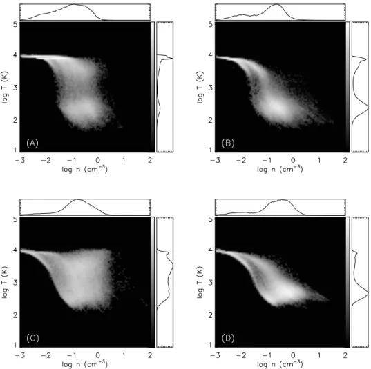
First we will compare the models A, B, C and D of section 2.4.1 without the effect of mechanical feedback. We let the model galaxy evolve, using the different ISM models as well as our star formation and SN feedback processes. Quickly, after about 200

(36)

Figure 2.12:Temperature-density distribution of simulation runs of model A, B, C and D w/o feedback. Histograms of the corresponding quantity are plotted to the right and above the frames. These histograms are linear and scaled to the maximum bin.

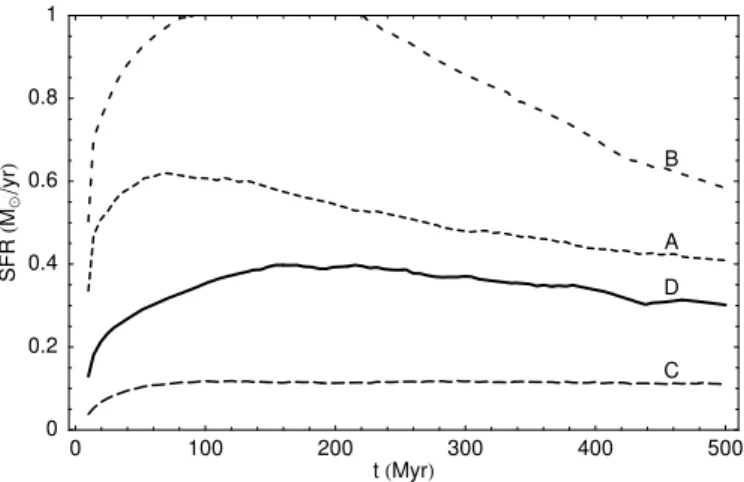
In Fig. 2.12 we have plotted the density-temperature diagram for the different models. If we look at the panel of model A, which is equivalent to the model of Gerritsen & Icke 1997, we recognize the two phase structure as found by them. Most of the gas is at temperatures of around T = 104 _{K. Note that gas cools to about}

T = 100K, but densities stay belown = 10cm−3_{, due to the limited resolution. The} star formation rate ofSFR≈0.6 M/yr is similar to that found by Gerritsen & Icke (Fig 2.13). We also find that the distribution of gas and stars has similar properties as in their simulations, more specifically: cold gas is confined to the midplane of the galaxy, showing a flocculent spiral structure caused by stretching of collapsing structures due to differential rotation.

Numerical studies of the interstellar medium on galactic scales

Numerical studies of the

interstellar medium on

Numerical studies of the

interstellar medium on

galactic scales

Proefschrift

Contents

Chapter 1

Introduction

1.1

Star forming galaxies

1.2

The challenge of modelling galaxies

1.2.1

The interstellar medium

1.2.2

Star formation and feedback

1.3

Outline of the thesis

1.4

Future Prospects

References

Chapter 2

Global models for the

interstellar medium

Abstract

2.1

Introduction

2.2

The N-body/SPH method

2.2.1

Barnes-Hut treecode

2.2.2

Smoothed Particle Hydrodynamics

2.2.3

Some notes on implementation

2.3

Physical processes of the ISM

2.3.1

Ionization

2.3.2

Cooling processes

2.3.3

Heating processes

2.3.4

Molecular gas

2.4

Equilibrium models

2.4.1

Heating and ionization assumptions

2.4.2

UV field and Cosmic rays

2.4.3

Varying chemical composition

2.5

Star formation and its effects

2.5.1

Star Formation

2.5.2

Stellar model

2.5.3

Feedback

2.6

Putting it all together

2.6.1

Initial conditions

2.6.2

Galaxy models without supernova feedback