Detection of low rank signals in noise and fast correlation mining with applications to large biological data

(1)

Detection of Low Rank Signals in Noise and Fast Correlation Mining

with Applications to Large Biological Data

Andrey A. Shabalin

A dissertation submitted to the faculty of the University of North Carolina at Chapel Hill in partial fulfillment of the requirements for the degree of Doctor of Philosophy in the Department of Statistics and Operations Research (Statistics).

Chapel Hill 2010

Approved by

Andrew B. Nobel, advisor Amarjit Budhiraja, reader Yufeng Liu, reader

(2)

(3)

ABSTRACT

ANDREY A. SHABALIN

Detection of Low Rank Signals in Noise and Fast Correlation Mining with Applications to Large Biological Data

(Under the direction of Andrew Nobel)

Ongoing technological advances in high-throughput measurement have given biomedical

researchers access to a wealth of genomic information. The increasing size and dimensionality

of the resulting data sets requires new modes of analysis. In this thesis we propose, analyze

and validate several new methods for the analysis of biomedical data. We seek methods that

are at once biologically relevant, computationally efficient, and statistically sound.

The thesis is composed of two parts. The first concerns the problem of reconstructing a

low-rank signal matrix observed in the presence of noise. In Chapter1 we consider the general reconstruction problem, with no restrictions on the low-rank signal. We establish a connection

with the singular value decomposition. This connection and recent results in random matrix

theory are used to develop a new denoising scheme that outperforms existing methods on a

wide range of simulated matrices.

Chapter2is devoted to a data mining tool that searches for low-rank signals equal to a sum of raised submatrices. The method, called LAS, searches for large average submatrices, also called

biclusters, using an iterative search procedure that seeks to maximize a statistically motivated

score function. We perform extensive validation of LAS and other biclustering methods on real

datasets and assess the biological relevance of their findings

The second part of the thesis considers the joint analysis of two biological datasets. In

Chap-ter 3 we address the problem of finding associations between single nucleotide polymorphisms (SNPs) and genes expression. The huge number of possible associations requires careful

atten-tion to issues of computaatten-tional efficiency and multiple comparisons. We propose a new method,

(4)

In Chapter 4we describe a method for combining gene expression data produced from dif-ferent measurement platforms. The method, called XPN, estimates and removes the systematic

differences between datasets by fitting a simple block-linear model to the available data. The

method is validated on real gene expression data.

(5)

ACKNOWLEDGEMENTS

I appreciate the enduring patience of my adviser Andrew Nobel, without him this

disserta-tion would be similar to the paper ofUpper(1974).

This work was supported, in part, by grants from Institutes of Health [grant numbers

P42-ES005948 and R01-AA016258], National Science Foundation [grant numbers DMS-0406361 and

DMS-0907177] National Cancer Institute Breast SPORE program to University of North

Car-olina at Chapel Hill [grant number P50-CA58223-09A1] National Cancer Institute [grant

num-ber RO1-CA-101227-01], and United States Environmental Protection Agency [grant numnum-bers

(6)

LIST OF FIGURES

1 LAS program user interface on left and FastMap on right. . . 7

1.1 Scree plot example. . . 9

1.2 Singular values of hard and soft thresholding estimates. . . 19

1.3 Relative performance of soft thresholding and OI oracle methods. . . 28

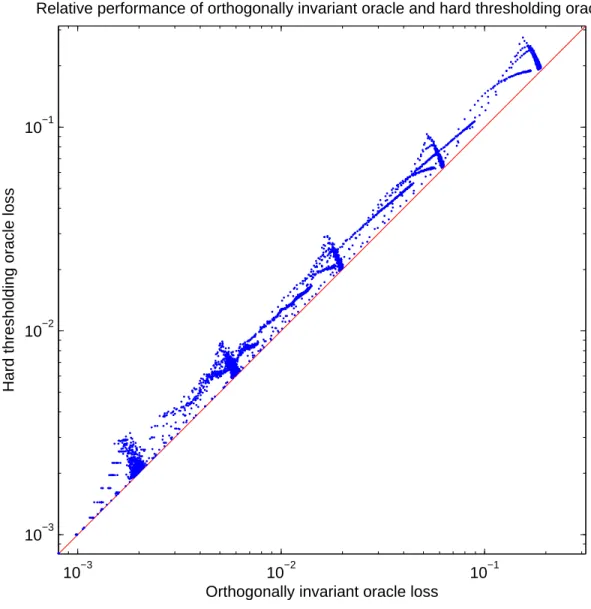
1.4 Relative performance of hard thresholding and OI oracle methods. . . 29

1.5 Relative performance of RMT method and OI oracle. . . 30

1.6 Largest singular values of the matched matrices from reconstruction and SPM. . 34

2.1 Illustration of bicluster overlap (left) and row-column clustering (right). . . 46

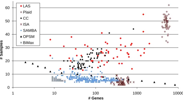
2.2 Bicluster sizes for different methods. . . 55

2.3 Best subtype capture of different biclustering and sample clustering methods. . . 61

2.4 Bar-plot of missed, true, and false discoveries for different biclustering methods.. 62

2.5 Classification error rates for SVM and the 5-nearest neighbor on “pattern” matrix. 66 3.1 Illustration of the Subset Summation Tree. . . 81

3.2 FastMap application GUI. . . 85

3.3 Fastmap timing for different number of genes and SNPs. . . 90

3.4 FastMap eQTL mapping results almost equivalent to those obtained with R/qtl. 92 3.5 SNP similarity matrix illustrating population stratification. . . 94

3.6 Strata median correction to improve transcriptome map. . . 96

4.1 Illustration of the block structure of the data. . . 100

4.2 Area between the CDFs of array mean minus array median across platforms. . . 106

4.3 Area between the CDFs of σ−M AD/Φ(0.75) for arrays of different platforms. . 106

4.4 AverageL2 distance from the samples of one study to the nearest from the other.107 4.5 Average correlation of arrays with their values before normalization. . . 108

4.6 Cross platform prediction error of the PAM classifier.. . . 110

(11)

LIST OF TABLES

1.1 AREL of different methods for square matrices. . . 31

1.2 AREL of different methods for rectangular matrices. . . 32

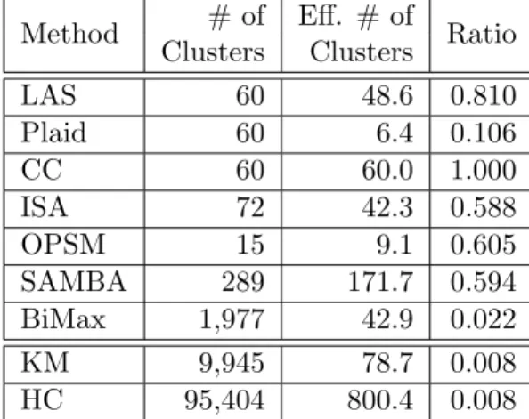
2.1 Output summary of different biclustering methods. . . 57

2.2 Average st.dev. and average pairwise correlation of gene and sample groups. . . . 58

2.3 Tests for survival, gene-set enrichment, and SAFE. . . 64

2.4 Discovery of multiple biclusters. . . 68

2.5 Summary table for 10 runs of LAS on the Hu data with different random seeds. . 69

2.6 Best subtype capture for 10 runs of LAS with different random seeds. . . 69

2.7 Stability of LAS tests for survival, and gene-set enrichment. . . 70

2.8 Summary statistics of LAS biclusters for data with added noise.. . . 71

2.9 Minus log10 p-values of best subtype capture for LAS on data with added noise. 71 2.10 Resistance of LAS tests for survival, and gene-set enrichment to noise. . . 72

3.1 FastMap eQTL mapping times. . . 89

3.2 FastMap tree construction and association mapping timings. . . 91

4.1 Gene correlation based tests. . . 110

(12)

INTRODUCTION

Rapid technological progress in the last decades has allowed biologists to produce

increas-ingly large data sets of various types. The first and most popular type is gene expression

mi-croarrays, which became popular back in 1990’s. Other technologies have developed to measure

micro-RNA expression and copy number variation, to detect single nucleotide polymorphisms

(SNPs), and even to perform full genome sequencing. The data sets produced by such

technolo-gies can often be represented as matrices of measurements, where each column corresponds to

a sample, and each row corresponds to a measured variable. Currently, large data sets can have

from tens of thousands (for gene expression arrays) to millions of variables (for SNP arrays).

The number of samples in the data sets can range from tens to thousands, the latter when the

efforts of multiple research centers is combined (see TCGA: The Cancer Genome Atlas). In

most cased the resulting data sets are real-valued. Although next generation sequencing arrays

generate integer values (counts), they can often be treated as real-valued. The clear exception

is SNP arrays, which contain binary values for inbred homozygous populations, and ternary

values for heterozygous populations like humans.

The analysis of biological data sets aims to reveal add information to our existing knowledge

about human diseases such as cancer or cystic fibrosis. For instance, breast cancer is now

known to be not one, but a family, of diseases that differ in speed of tumor growth, response to

treatments, likelihood of metastases, and likelihood of relapse after surgical removal of a tumor.

Gene expression technology enabled biologists to discover subtypes of breast and other types

of cancer. SNP data can be used to determine how differences in genotype predispose people

to different diseases and types of diseases. Genotypic differences between individuals can be

associated with various phenotypes, including phenotypes derived from clinical variables and

(13)

targeting individuals genetic makeup.

Typical gene expression data set has tens of thousands of variables and hundreds of samples.

SNP arrays have millions of variables. Even preliminary analysis of such large datasets is

complicated by their size. While a simple visual inspection of gene expression data is now

common, it is not practical for SNP data. Preliminary analysis by simply looking at the table

of numbers is not possible even for moderately sized data sets, as they contain millions of

measurements. The common approach to visualizing gene expression data is the following.

The rows and columns of the data matrix are hierarchically clustered, and then reordered so

that the clusters contiguous. Next, a heatmap is produced. In heatmap each measurement is

represented by just one pixel, colored green for negative values, red for positive, with brightness

proportional to the absolute value of the measurement. SNP data sets are usually not visualized

in this way, as they have too many variables. Instead, scientists perform an analysis first, and

then visualize the results of the analysis in some way. For example, one can evaluate association

of each SNP with a response variable, like survival, and plot the association statistics for SNPs

in the region near the SNP with the largest association.

Analysis of large biological datasets must be both computationally efficient and statistically

principle. For instance, if a method is statistically motivated, but has complexity proportional

to the cube of the number of variables, it would be impractical or even unfeasible for many

data sets. Such methods may perform well when tested on data sets with 500 to 1000 variables,

but they would not scale well to modern data sets with tens to hundreds of thousands of

variables. On the other hand, some existing methods for the analysis of biological data sets

are computationally efficient, but lack statistical justification. For instance, some data mining

methods are designed to find all patterns in a given data set that satisfy a certain criterion,

regardless of how likely it is to find such patterns in a matrix of pure noise. For this reason

such methods may produce a large output with many spurious findings. Others may have

some statistical motivation, but fail to account for multiple comparisons. Some data mining

methods assess significance of their findings by calculating the probability of such exact pattern

appearing in a random data matrix. However, there is usually a great number of patterns the

(14)

Another, less widely recognized problem of some methods lies in the number of parameters

they have. The method can be hard to apply if the parameters have to be individually

hand-picked for each dataset. Moreover, if a generalization of an existing method is proposed, which

adds more parameters, one can always choose the parameters for the new method to outperform

the old method on any given test. However, this does not indicate that the new method would

be better in practice, when the choice of all the parameters would become a problem, not an

advantage.

Last but not least, methods that do not have the drawbacks listed above sometimes lack

validation on real data. For example, methods for mining biological data sets, may search for

particular features of the data in both computationally efficient and statistically sound fashion,

but not be actually useful for a biologist.

In this dissertation we propose several new statistical methods for analysis of biological

data sets, each computationally efficient, statistically principal, and validated on real data.

In Section 2 we propose a new biclustering method, called LAS. The LAS section contain a revised version of the paper published in Annals of Applied Statistics (Shabalin, Weigman,

Perou & Nobel 2009). Next, in Section 3 we present a new method for fast eQTL analysis, called FastMap. The FastMap section contain a revised and extended version of the paper

published in Bioinformatics (Gatti, Shabalin, Lam, Wright, Rusyn & Nobel 2009). In Section4 we present a new method for cross platform normalization of gene expression arrays, called

XPN. The XPN section contain a revised version of the paper published in Bioinformatics

(Shabalin, Tjelmeland, Fan, Perou & Nobel 2008). The dissertation begins with Chapter 1 which presents our most recent research and most theoretical research. It studies the problem

of recovery of denoising of low-rank matrices. This research has not yet been submitted to any

journal.

Outline

In Chapter1we present a new method for denoising of low-rank matrices with additive Gaussian noise. The denoising problem is usually solved by singular value decomposition of the observed

data matrix followed by shrinkage or thresholding of its singular values. Although a wide

(15)

reconstruction scheme must indeed be based on the singular value of the observed matrix. Even

more, it should only change the singular value of the matrix, leaving the singular vectors intact.

However, as we determine in latter in the Chapter, it is not efficient to restrict the scheme to

simple shrinkage and/or thresholding of singular values.

Next, applying random matrix theory we study the effect of noise on low rank matrices,

namely on their singular values and singular vectors. Then we construct the proposed denoising

scheme based on this knowledge.

Simulation study with a wide range of settings shows that the proposed reconstruction

scheme strongly outperforms the conventional ones regardless of the choice of shrinking and

thresholding parameters for them. The performanceof the proposed method nearly matches

the performance of the general oracle denoising scheme.

As a side result we determine the minimum strength (singular value) the signal must have

to be at least partially recoverable.

In Chapter2we present a new data mining method called LAS. It was inspired by the process of visual mining of heatmap data representations. Some biologists visually inspect heatmaps of

gene expression data in search of solid red or green blocks. Such blocks represent sample-variable

interactions, sets of gene that are simultaneously active or inactive for corresponding sets of

samples. LAS approach a more general problem of finding submatrices with large positive or

negative average. Such submatrices do not have to be contiguous in any heatmap representation

of the data. To search for such submatrices, called biclusters, we first assign each submatrix

a score, which is larger for larger and brighter submatrices. The score is defined as negative

logarithm of p-value, calculated for the null model that data has only noise and Bonferroni

corrected for the number of submatrices of given size. Biclusters with larger score are found

first. Once a bicluster is found, it is removed by reducing its elements, and the search continues

for the next ones.

The task of finding a bicluster with largest score is NP-complete, so we use a heuristic

algo-rithm for the search. Our simulations have shown that LAS algoalgo-rithm is most often successful

in finding raised submatrices in simulated data.

(16)

to breast and lung cancer data sets. We found at least one bicluster for each known cancer

subtype those sample set closely matches the samples of the subtype. We have also tested the

biclusters’ sample sets for association with clinical variables and gene sets for overrepresentation

of know gene categories. In all tests LAS outperforms other known biclustering methods.

The LAS problem can be seen as a special case of signal detection problem. LAS model

assumes the signal in the observed data to be a sum of matrices, each equal to a fixed number

on a submatrix and zero elsewhere. Note that the signal matrix withB biclusters has rank at

most B, so the LAS model is a particular case of low-rank signal detection model considered

in Chapter 1. However, as we show in Section 2.6.1, LAS algorithm can find submatrices that are not detectable with SVD of the data matrix.

Although the analysis of individual datasets has proven to be useful, more information can

be discovered by joint analysis of two, or more datasets. A particular case of such analysis is

gene expression quantitative trait loci (eQTL) mapping, which searches for associations between

SNPs and genes. The number of associations to be calculated is equal to the product of the

number of SNPs (>1m) and the number of genes measured (∼40k), which can be in the order of

tens of billions. The computational burden is even greater if the researcher chooses to perform

permutation analysis to assess the significance of their findings. To address the computational

issues while keeping the analysis statistically correct, we propose a new computational method

for eQTL analysis, called FastMap. The method exploits the discrete structure of SNP data

(whether binary or ternary) to greatly improve the speed of the eQTL analysis. FastMap

performs analysis on gene by gene basis. The significance of the strongest association of a given

gene expression with the available SNPs is assessed using a permutation approach. By assessing

the significance of the strongest association over all SNPs we avoid multiple comparison issue

across SNPs. In order to address multiple comparisons across genes, FastMap assigns a q-value

(Storey & Tibshirani 2003) assessing false discovery rate to each gene.

The original FastMap program, as published in Gatti et al. (2009), was designed to work

with homozygous SNP data only. Since then, the program has been improved, it now supports

(17)

Collaboration of different cancer centers allows biologist to combine data in order to gain

better strength in the subsequent analysis. More and more datasets become publicly available

with time. However one can not simply join datasets from different sources. The data produced

by different research centers differs more than the data produced within one center. This

difference can arise from a variety of reasons. First, different studies may use gene expression

arrays from different manufacturers, or different versions of arrays from the same manufacturer.

Second, even measurements from various batches of samples from the same array can differ

more than the measurements within each batch. Differences across batches occur because of

differences in measuring conditions, including different batches of arrays, batches of reagents,

and different versions of processing software. Differences across platforms occur because the

probes of different arrays may target different sequences from the the same genes, which are

often located in different exons.

To remove batch and/or platform effects across gene expression datasets we propose a new

method for cross platform normalization, called XPN. It is based on a block model of the data.

XPN is distinguished from other platform normalization methods that are gene-wise linear. In

Chapter 4 we describe the method and carefully validate it on several real data. The tests on real data show that XPN is more successful in removing platform effects while preserving

important biological information.

Software

For the LAS, FastMap, and XPN methods presented in this dissertation we provide free

imple-mentations of the methods.

The LAS program is implemented in C# programming language with an intuitive graphics

user interface (see Figure 1, left). An alternative implementation in Matlab is also available for those who may want to add modifications to the code and for cross-platform compatibility.

The LAS software is available at https://genome.unc.edu/las/.

The FastMap method is implemented in Java. It also has an easy to navigate graphical

user interface (see Figure 1, right). The FastMap program and source code are available at http://cebc.unc.edu/fastmap86.html.

(18)

Figure 1: LAS program user interface on left and FastMap on right.

(19)

CHAPTER 1

Reconstruction of a Low-rank Matrix in the

Presence of Gaussian Noise

1.1 Introduction

This chapter addresses the problem of recovering a low rank matrix whose entries are observed

in the presence of additive Gaussian noise.

Problems of this sort appear in multiple fields of study including compressed sensing and

image denoising. In many of these cases the signal matrix is known to have low rank. For

example, a matrix of squared distances between points in d-dimensional Euclidean space is

know to have rank at most d+ 2. A correlation matrix for a set of points in d-dimensional

Euclidean space has rank at mostd. In other cases the target matrix is often assumed to have

low rank , or to have a good low-rank approximation. For example,Alter et al.(2000),Holter

et al. (2000) andRaychaudhuri et al. (2000) assumed the signal component of gene expression

matrices to have low rank.

The reconstruction problem considered here has a signal plus noise structure. Our goal is

to recover an unknown m×n matrix A of low rank that is observed in the presence of i.i.d.

Gaussian noise as matrix Y:

Y = A+√σ

nW, where Wij ∼ i.i.d. N(0,1).

In what follows, we first consider the variance of the noise σ2 to be known and assume it to

(20)

observed matrix Y. Then, the largest singular values are visually inspected on a scree plot. A

sample scree plot is shown in Figure 1.1 below. The rank R of the signal is then estimated as the number of singular values to the left of the ’elbow’ point. The scree plot on Figure 1.1 clearly indicates a rank-2 signal. The signal is then estimated as the sum of first R terms in

the singular value decomposition of Y.

0 2 4 6 8 10 12 14 16 18 20 50

60 70 80 90 100 110

Singular values

Figure 1.1: Scree plot for a 1000×1000 rank 2 signal matrix with noise.

A more formal version of this approach is known as hard thresholding. Hard thresholding

estimates the signal matrix A by arg min_B_:_rank₍_B₎₌_RkY −Bk2

F for some data-driven choice of rank R. Hard thresholding preserves first R singular values of the matrix Y, and sets the

rest to zero. Hard thresholding can be viewed equivalently as a minimization problem with

rank-based penalty

arg min B

kY −Bk2_F +λ2rank(B) ,

for some parameterλ. Here and in what followsk · kF denote Frobenius norm of a matrix.

Another approach is to shrink, not threshold the singular values of the observed matrix. It

reduces all singular values by a constant λand sets all singular values smaller that λequal to

zero. Such approach is called soft thresholding and it can also be formulated as minimization

problem: arg minBkY −Bk2F + 2λkBk∗, where λ is a parameter and k · k∗ is matrix nuclear norm (sum of singular values).

Both hard and soft thresholding methods are studied in the literature and various rules for

selection of the penalization parameters are proposed, some with performance guaranties under

certain conditions. Both these approaches are based on SVD of the data and are popular in

practical applications. For instance, Wall et al. (2001), Alter et al. (2000), and Holter et al.

(21)

applied SVD to impute missing values. SVD is also used for image denoising. However a better

performance is achieved when SVD is applied to small blocks of pixels, not to the whole image.

Denoising methods of Wongsawat et al. and Konstantinides et al. (1997) perform SVD on

square subblocks and set to zero the singular values smaller than some threshold.

However, it is natural to ask whether SVD-based approach is optimal. In general, a

re-construction scheme is a map g : Rm×n → Rm×n. It does not have to be based on SVD of

matrix Y and does not have to be formulated as a penalized minimization problem. It even

does not have to produce matrices of low rank. Can we achieve better reconstruction if we do

not restrict ourselves to scheme that just shrink or threshold singular values? Can we achieve

a better reconstruction if we do not restrict ourselves to the method based on SVD and which

produce low-rank matrices?

In the first part of this chapter we analyze the matrix reconstruction problem and determine

several necessary properties of efficient reconstruction schemes. In Section 1.2 we prove that under mild conditions on the prior information about the signal (lack of information about its

singular vectors) any effective denoising scheme must be based on the singular value

decompo-sition (SVD) of the observed matrix. Moreover, it need only modify the singular values, not

singular vectors. These facts alone reduce the space of efficient reconstruction schemes from

g:Rm×n→Rm×n to justg:Rm∧n→Rm∧n, wherem∧n denotes the minimum ofm andn.

In the second part of the chapter we propose a new reconstruction scheme. Rather than

adopting approaches of hard and soft thresholding, we start by determining the effect of additive

noise on the singular values and singular vectors of low-rank matrices. We do it by first making a

connection between the matrix reconstruction problem and spiked population models in random

matrix theory. In Section 1.5 we translate relevant theorems from random matrix theory to the settings of the matrix reconstruction problem. The proposed reconstruction scheme is then

derived from these results in Section1.6. The proposed scheme is designed to reverse the effect of the noise on the singular values of the signal and corrects for the effect of the noise on the

signal’s singular vectors. We call the proposed method RMT for on its use of random matrix

theory.

(22)

versions of the existing methods, and closely matches the performance of a general oracle scheme

for generated matrices of various size and signal spectra.

1.2 The Matrix Reconstruction Problem

1.2.1 Statement of the Problem

The reconstruction problem considered here has a signal plus noise structure common to many

estimation problems in statistics and signal processing. Our goal is to recover an unknown

m×nmatrixAof low rank that is observed in the presence of Gaussian noise. Specifically, we

consider the matrix additive model

Y = A+√σ

nW (1.1)

where Y denotes the observed matrix, σ >0 is an unknown variance parameter, and W is a

Gaussian random matrix with independentN(0,1) entries. The matricesY,A, andW are each

of dimensionm×n. The factorn−1/2 ensures that the signal and noise are comparable, and is essential for the for the asymptotic study of matrix reconstruction in Section 1.5, but it does not play a critical role in the characterization of orthoginally invariant schemes that follows.

At the outset we will assume that the variance σ is known and equal to one. In this case

the model (1.1) simplifies to

Y = A+ √1

nW, Wij independent ∼ N(0,1). (1.2)

Formally, a matrix recovery scheme is a mapg:Rm×n→Rm×nfrom the space ofm×nmatrices

to itself. Given a recovery scheme g(·) and an observed matrix Y from the model (1.2), we regard Ab =g(Y) as an estimate of A. Recall that the squared Frobenius norm of an m×n

matrixB ={bij} is given by

kBk2_F = m X

i=1

n X

j=1

b2_ij.

If the vector space Rm×n is equipped with the inner product hA, Bi= tr(A0B), then it is easy

to see that kBk2

(23)

Frobenius norm

Loss(A,Ab) = kAb−Ak2_F. (1.3)

Remark: Our assumption that the entries of the noise matrix W are Gaussian arises from two conditions required in the analysis that follows. The results of Section1.3 require thatW

has an orthogonally invariant distribution (see Definition 3). On the other hand, the results of Section 1.5 are based on theorems from random matrix theory, which require the elements of

W to be i.i.d. with zero mean, unit variance, and finite forth moment. It is known that the only

distribution satisfying both these assumptions is the Gaussian (Bartlett 1934). Nevertheless,

our simulations (not presented) show that the Gaussian noise assumption is not required to

ensure good performance of the RMT reconstruction method.

In the next section we will provide some insights to the structure of the reconstruction

problem.

1.3 Invariant Reconstruction Schemes

The additive model (1.2) and Frobenius loss (1.3) have several elementary invariance properties, which lead naturally to the consideration of reconstruction methods with analogous forms of

invariance. Recall that a square matrix U is said to be orthogonal if U U0 = U0U = I, or equivalently, if the rows (or columns) of U are orthonormal. If we multiply each side of (1.2) from the left right by orthogonal matricesU and V0 of appropriate dimensions, we obtain

U Y V0 = U AV0 + √1

nU W V

0_. _(1.4)

Proposition 1. Equation (1.4) is a reconstruction problem of the form (1.2) with signalU AV0

and observed matrixU Y V0. IfAbis an estimate ofA in model (1.2), then UAVb 0 is an estimate

of U AV0 in model (1.4) with the same loss.

Proof. If A has rank r then U AV0 also has rank r. To prove the first statement, it remains

(24)

let U and V be the orthogonal matrices in (1.4). For anym×nmatrixB,

kU Bk2_F = tr(U B)0(U B) = trB0B = kBk2_F,

and more generallykU BV0k2

F =kBk2F. Applying the last equality toB =Ab−A yields

Loss(U AV0, UAVb 0) = kU(Ab−A)V0k2_F = kAb−Ak2_F = Loss(A,Ab)

as desired.

In light of Proposition 1it is natural to consider reconstruction schemes that are invariant under orthogonal transformations of the observed matrix Y.

Definition 2. A reconstruction scheme g(·) is orthogonally invariant if for any m×nmatrix

Y, and any orthogonal matrices U and V of appropriate size, g(U Y V0) =U g(Y)V0.

In general, a good reconstruction method need not be orthogonally invariant. For example,

if the target matrix A is known to be diagonal, then for each Y the estimate g(Y) should be

diagonal as well, and in this case g(·) is not orthogonally invariant. However, as we show in

the next theorem, if we have no information about the singular vectors of A (either prior or

from the singular values ofA), then it suffices to restrict our attention to orthogonally invariant

reconstruction schemes.

Definition 3. A random m×nmatrixZ has an orthogonally invariant distribution if for any

orthogonal matrices U and V of appropriate size the distribution of U ZV0 is the same as the

distribution of Z.

As noted above, a matrix with independent N(0,1) entries has an orthogonally invariant

distribution. If Z has an orthogonally invariant distibution, then its matrix of left (right)

singular vectors is uniformly distributed on the space of m×m (n×n) orthogonal matrices.

Theorem 4. Let Y = A+W, where A is a random target matrix. Assume that A and W

are independent and have orthogonally invariant distributions. Then, for every reconstruction

scheme g(·), there is an orthogonally invariant reconstruction scheme ˜g(·) whose expected loss

(25)

Proof. LetU be anm×mrandom matrix that is independent of Aand W, and is distributed according to Haar measure on the compact group ofm×morthogonal matrices. Haar measure

is (uniquely) defined by the requirement that, for every m ×m orthogonal matrix C, both

CU and UC have the same distribution as U (c.f. (Hofmann & Morris 2006)). Let V be an

n×nrandom matrix distributed according to the Haar measure on the compact group ofn×n

orthogonal matrices that is independent ofA, W and U. Given a reconstruction scheme g(·), define a new reconstruction scheme

˜

g(Y) = E[U0g(UYV0)V|Y].

It follows from the definition ofUandV that ˜g(·) is orthogonally invariant. The independence of{U,V}and{A, W}ensures that conditioning onY is equivalent to conditioning on{A, W}, which yields the equivalent representation

˜

g(Y) = E[U0g(UYV0)V|A, W].

Therefore,

ELoss(A,˜g(Y)) = EE[U0g(UYV0)V−A|A, W]

2

F ≤ EkU0g(UYV0)V−Ak2F

= Ekg(UYV0)−UAV0k2F.

The inequality above follows from the conditional version of Jensen’s inequality applied to each

term in the sum defining the squared norm. The final equality follows from the orthogonality

of U andV. The last term in the previous display can be analyzed as follows:

Eg(UYV0)−UAV0

2

F = E h

E kg(UAV0+n−1/2UWV0)−UAV0k2F |U,V,A i

= E

h

E kg(UAV0+n−1/2W)−UAV0k2F|U,V,A i

= Eg(UAV0+n−1/2W)−UAV0

2

F.

(26)

the independence of W and U,A,V, and the orthogonal invariance of L(W). By a similar argument, using the orthogonal invariance of L(A), we have

Ekg(UAV0+n−1/2W)−UAV0k2F = E h

E kg(UAV0+n−1/2W)−UAV0k2F|U,V, W i

= E

h

E kg(A+n−1/2W)−Ak2F|U,V, W i

= Ekg(A+n−1/2W)−Ak2F. The final term above is ELoss(A, g(Y)). This completes the proof.

In what follows we will restrict our attention to orthogonally invariant reconstruction

schemes.

1.3.1 Singular Value Decomposition

A natural starting point for reconstruction of a target matrixAis the singular value

decomposi-tion (SVD) of the observed matrixY. The SVD ofY is intimately connected with orthogonally

invariant reconstruction methods. Recall that the singular value decomposition of an m×n

matrixB is given by the factorization

B = U DV0 = m∧n

X

j=1

djujv0j.

HereU is an m×m orthogonal matrix with columnsuj,V is ann×northogonal matrix with

columnsvj, andDis anm×nmatrix with diagonal entriesDjj =dj ≥0 forj= 1, . . . , m∧n, and

all other entries equal to zero. The numbersd1 ≥d2 ≥...≥dm∧n≥0 are the singular values ofB. The columnsuj (andvj) are the left (and right) singular vectors ofB. Although it is not

necessarily square, we will refer toD as a diagonal matrix and writeD= diag(d1, . . . , dm∧n). An immediate consequence of the SVD is thatU0BV =D, so we can diagonalizeBby means of left and right orthogonal multiplications. The next proposition follows from our ability to

diagonalize the target matrixA in the reconstruction problem.

Proposition 5. Let Y =A+n−1/2_W_{, where} _W _{has an orthogonally invariant distribution. If}

g(·) is an orthogonally invariant reconstruction scheme, then for any fixed target matrix A, the

(27)

values of A.

Proof. LetU DAV0be the SVD ofA. ThenDA=U0A V, and as the Frobenius norm is invariant

under left and right orthogonal multiplications,

Loss(A, g(Y)) = kg(Y)−Ak2_F = kU0(g(Y)−A)V k2_F

= kU0g(Y)V −U0AV k_F2 = kg(U0Y V)−DAk2F = kg(DA+n−1/2U0W V)−DAk2F.

The result now follows from the fact that U W V0 has the same distribution as W.

We now address the implications of our ability to diagonalize the observed matrix Y. Let

g(·) be a orthogonally invariant reconstruction method, and let U DV0 be the singular value decomposition ofY. It follows from the orthogonal invariance ofg(·) that

g(Y) = g(U DV0) = U g(D)V0 = m X

i=1

n X

j=1

cijuivj0 (1.5)

where cij depend only on the singular values of Y. In particular, any orthogonally invariant

g(·) reconstruction method is completely determined by how it acts on diagonal matrices. The

following theorem allows us to substantially refine the representation (1.5).

Theorem 6. Let g(·) be an orthogonally invariant reconstruction scheme. Then g(Y) is

diag-onal whenever Y is diagonal.

Proof. Assume without loss of generality that m≥n. Let the observed matrixY be diagonal,

Y = diag(d1, d2, ..., dn), and let Ab = g(Y) be the reconstructed matrix. Fix a row index

1 ≤ k ≤ m. We will show that Ab_kj = 0 for all j 6=k. Let D_L be an m×m matrix derived

from the identity matrix by flipping the sign of the kth _{diagonal element.} _{More formally,}

DL = I−2eke0k, whereek is thekth standard basis vector inRm. The matrixDLis known as a Householder reflection.

Let DR be the top left n×n submatrix of DL. Clearly DLD0L = I and DRDR0 = I, so bothDLandDRare orthogonal. Moreover, all three matricesDL, Y,andDRare diagonal, and

(28)

g(·) that

b

A = g(Y) = g(DLY DR) = DLg(Y)DR = DLA Db _R.

The (i, j)th element of the matrix DLA Db _R is Ab_ij(−1)δik(−1)δjk, and therefore Ab_kj =−Ab_kj if

j6=k. Askwas arbitrary,Abis diagonal.

As an immediate corollary of Theorem6and equation (1.5) we obtain a compact, and useful, representation of any orthogonally invariant reconstruction scheme g(·).

Corollary 7. Let g(·) be an orthogonally invariant reconstruction scheme. If the observed

matrix Y has singular value decomposition Y =P

djujv_j0 then the reconstructed matrix

b

A = g(Y) = m∧n

X

j=1

cjujvj0, (1.6)

where the coefficients cj depend only on the singular values of Y.

The converse of Corollary 7is true under a mild additional condition. Let g(·) be a recon-struction scheme such thatg(Y) =cjujv0_j, wherecj =cj(d1, . . . , dm∧n) are fixed functions of the

singular values ofY. If the functions{cj(·)}are such thatci =cj wheneverdi=dj, theng(·) is

orthogonally invariant. This follows from the uniqueness of the singular value decomposition.

1.4 Hard and Soft Thresholding

Let Y be an observed m×n matrix with singular value decomposition Pm∧n

j=1 djujvj0. Many reconstruction schemes act by shrinking the singular values of the observed matrix towards zero.

Shrinkage is typically accomplished by hard or soft thresholding. Hard thresholding schemes set

every singular value of Y less than a positive threshold λequal to zero, leaving other singular

values unchanged. The family of hard thresholding schemes is defined by

g_λH(Y) = m∧n

X

j=1

(29)

Soft thresholding schemes subtract a positive numberνfrom each singular value, setting values

less thanν equal to zero. The family of soft thresholding schemes is defined by

g_νS(Y) = m∧n

X

j=1

(dj−ν)+ujvj0, whereν >0.

Hard and soft thresholding schemes can be defined equivalently in the respective penalized

forms

gH_λ(Y) = arg min B

kY −Bk2

F +λ2rank(B)

gS_ν(Y) = arg min B

kY −Bk2_F + 2νkBk∗ .

In the second display, kBk∗ denotes the nuclear norm of B, equal to the sum of its singular

values.

In practice, hard and soft thresholding schemes require estimates of the noise variance,

as well as the selection of appropriate cutoff or shrinkage parameters. There are numerous

methods in the literature for choosing the hard threshold λ. Heuristic methods often make

use of the scree plot, which displays the singular values of Y as a function of their rank: λ

is typically chosen to be the y-coordinate of a well defined “elbow” in the plot. In recent

work, Bunea et al. (2010) propose a specific choice of λ and provide performance guaranties

for the resulting hard thresholding scheme using techniques from empirical process theory and

complexity regularization. Selection of the soft thresholding shrinkage parameterν may also be

accomplished by a variety of methods. Negahban & Wainwright(2009) propose a specific choice

of ν and provide performance guarantees for the resulting soft thresholding scheme. Hard and

soft thresholding schemes are orthogonally invariant if the estimates of λand ν, respectively,

depend only on the singular values ofY.

1.5 Asymptotic Approach

The families of hard and soft thresholding methods described above include many existing

reconstruction schemes. Both thresholding approaches seek low rank (sparse) estimates of the

target matrix, both can be naturally formulated as optimization problems, and under mild

(30)

all orthogonally invariant reconstruction schemes encompasses a much broader class of possible

reconstruction procedures, and it is natural to consider alternatives to thresholding that may

offer better performance.

0 10 20 30 40 50 60 70 80 90 100 0

1 2 3 4 5

500 x 500 Matrix, Rank 50 Signal Singular values of A Singular values of Y Best hard thresholding

0 10 20 30 40 50 60 70 80 90 100 0

1 2 3 4 5

500 x 500 Matrix, Rank 50 Signal Singular values of A Singular values of Y Best soft thresholding

Figure 1.2: Singular values of hard and soft thresholding estimates.

Figure 1.2 illustrates the action of hard and soft thresholding on a 500×500 matrix with a rank 50 signal. The blue line marks the singular values of the signal A and the green line

marks the those of the observed matrixY. The plots show the singular values of the hard and

soft thresholding estimates incorporating the best choice of parameters λ and ν, respectively.

Clearly, neither thresholding scheme delivers an accurate estimate of the original singular values

(or the original matrix). Moreover, the figures suggest that a hybrid scheme that combines soft

and hard thresholding might offer better performance. We construct an improved reconstruction

scheme in a principled fashion, by studying the effect of noise on low-rank signal matrices. The

key tools in this analysis are several recent results from random matrix theory.

Random matrix theory is broadly concerned with the spectral properties of random

ma-trices, and is an obvious starting point for an analysis of matrix reconstruction. The matrix

reconstruction problem has several points of intersection with random matrix theory. Recently

a number of authors have studied low rank deformations of Wigner matrices (Capitaine et al.

2009,Féral & Péché 2007,Maıda 2007,Péché 2006). However, their results concern symmetric

matrices, a constraint not present in the reconstruction model, and are not directly applicable

to the reconstruction problem of interest here. (Indeed, our simulations of non-symmetric

ma-trices exhibit behavior deviating from that predicted by the results of these papers.) A signal

plus noise framework similar to matrix reconstruction is studied inDozier & Silverstein(2007),

(31)

matrix (Dozier & Silverstein) or recovery of the singular values of the signal (Nadakuditi &

Silverstein), and do not consider the more general problem of reconstruction.

Our proposed denoising scheme is based on the theory of spiked population models in

ran-dom matrix theory. Using existing results on spiked population models, we establish asymptotic

connections between the singular values and vectors of the target matrix A and those of the

observed matrixY. These asymptotic connections provide us with finite-sample estimates that

can be applied in a non-asymptotic setting to matrices of small or moderate dimensions.

1.5.1 Asymptotic Matrix Reconstruction Model

The proposed reconstruction method is based on an asymptotic version of the matrix

recon-struction problem (1.2). For n≥1 let integers m=m(n) be defined in such a way that

m

n → c > 0 as n→ ∞. (1.7)

For eachnlet Y,A, andW bem×nmatrices such that model (1.2) holds:

Y = A+√1

nW, (1.8)

where the entries ofW are independentN(0,1) random variables. We assume that the target

matrixAhas fixed rankr ≥0 and fixed non-zero singular valuesλ1(A), . . . , λr(A) that are are

independent ofn. The constant crepresents the limiting aspect ratio of the observed matrices

Y. The scale factor n−1/2 ensures that the singular values of the target matrix are comparable to those of the noise. Model (1.8) matches the asymptotic model used by Capitaine et al.

(2009),Féral & Péché (2007) in their study of fixed rank perturbations of Wigner matrices.

In what follows λj(B) will denote the j-th singular value of a matrix B, and uj(B) and

vj(B) will denote, respectively, the left and right singular values corresponding toλj(B). Our

first proposition concerns the behavior of the singular values ofY when the target matrixA is

equal to zero.

Proposition 8. Under the asymptotic reconstruction model with A = 0 the empirical

(32)

distribution with density

fY(s) =

s−1

π(c∧1) p

(a−s2₎₍_s2₋_b₎_, _s_∈_[√_a,√_b_]_, _(1.9)

wherea= (1−√c)2 andb= (1 +√c)2. Moreover,λ1(Y)

P

−→ 1 +√candλm∧n(Y) P

−→ 1−√c

as n tends to infinity.

The existence and form of the density fY(·) are a consequence of the classical Marˇ

cenko-Pastur theorem (Marˇcenko & Pastur 1967,Wachter 1978). The in-probability limits ofλ1(Y)

and λm∧n(Y) follow from later work of Geman (1980) and Wachter (1978), respectively. If

c = 1, the density function fY(s) simplifies to the quarter-circle law fY(s) = π−1 √

4−s2 _for

s∈[0,2].

The next two results concern the limiting eigenvalues and eigenvectors of Y when A is

non-zero. Proposition 9 relates the limiting eigenvalues of Y to the (fixed) eigenvalues of A, while Proposition 10 relates the limiting singular vectors of Y to the singular vectors of A. Proposition 9 is based on recent work of Baik & Silverstein (2006), while Proposition 10 is based on recent work of Paul (2007), Nadler(2008), andLee et al. (2010). The proofs of both

results are given in Section1.8.2.

Proposition 9. Let Y follow the asymptotic matrix reconstruction model (1.8) with target

singular valuesλ1(A)≥...≥λr(A)>0. For 1≤j≤r, as n tends to infinity,

λj(Y) −→P       

1 +λ2_j(A) +c+_λ2c

j(A)

1/2

if λj(A)> 4

√

c

1 +√c if 0< λj(A)≤ 4

√

c

The remaining singular values λr+1(Y), . . . , λm∧n(Y) of Y are associated with the zero

singu-lar values of A: their empirical distribution converges weakly to the limiting distribution in

Proposition 8.

Proposition 10. Let Y follow the asymptotic matrix reconstruction model (1.8) with distinct

target singular values λ1(A)> λ2(A)> ... > λr(A)>0. Fix j such thatλj(A)> 4

√

(33)

n tends to infinity,

uj(Y), uj(A)2 −→P 1− c

λ4

j(A)

1 + c

λ2

j(A)

and

vj(Y), vj(A) 2 P

−→ 1− c

λ4

j(A)

1 + 1

λ2

j(A)

Moreover, if k 6=j, 1 ≤k ≤r then hui(Y), uk(A)i

P

−→ 0 and hvi(Y), vk(A)i P

−→ 0 as n tends

to infinity.

The limits established in Proposition 9 indicate a phase transition. If the singular value

λj(A) is less than or equal to 4 √

cthen, asymptotically, the singular valueλj(Y) lies within the

support of the Marˇcenko-Pastur distribution and is not distinguishable from the noise singular

values. On the other hand, if λj(A) exceeds √4_c _{then, asymptotically,} _λ

j(Y) lies outside the support of the Marˇcenko-Pastur distribution, and the corresponding left and right singular

vectors ofY are associated with those of A (Proposition10).

1.6 Proposed Reconstruction Scheme

Let Y be an observed m×n matrix generated from the additive model Y = A+n−1/2σW. Assume for the moment that the varianceσ2of the noise is known, and equal to one. Estimation

of σ is discussed in the next subsection. Let

Y =

m∧n X

j=1

λj(Y)uj(Y)v0j(Y)

be the SVD ofY. Following the discussion in Section1.3, we seek an estimate ofAof the form

b

A =

m∧n X

j=1

cjuj(Y)v0j(Y),

where each coefficientcj depends only on the singular valuesλ1(Y), . . . , λm∧n(Y) of Y.

Our proposed reconstruction scheme is derived from the limiting relations in Propositions

(34)

ity relations. Suppose that the singular values and vectors of A are known. Then we seek

coefficients {cj}minimizing

Loss(A,Ab) =

m∧n X

j=1

cjuj(Y)v0j(Y) − m∧n

X

j=1

λj(A)uj(A)v0j(A)

2

F.

Phase transition phenomenon (Proposition9) indicated that we can restrict the first sum to the first r0 = #{j :λj(A) > 4

√

c} elements. By definition of A only first r elements of the second

sum are non-zero, so

Loss(A,Ab) =

r0

X

j=1

cjuj(Y)vj0(Y) − r X

j=1

λj(A)uj(A)v_j0(A)

2

F

Proposition 10 ensures that the left singular vectors ui(Y) and uk(A) are asymptotically orthogonal if i6=k, i≤r0, k≤r, and therefore

Loss(A,Ab) l = r0 X j=1

c_ju_j(Y)v0_j(Y) − λ_j(A)u_j(A)v_j0(A)

2

F.

Fix 1≤j ≤r0. Expanding the j-th term in the above sum gives

λ_j(A)u_j(A)v_j0(A) − c_ju_j(Y)v_j0(Y)

2

F = c2_ju_j(Y)v0_j(Y)

2

F + λ

2

j(A)

uj(A)v_j0(A)

2

F − 2cjλj(A)

uj(A)v0j(A), uj(Y)vj0(Y)

= λ2_j(A) + c_j2 − 2cjλj(A)

uj(A), uj(Y) vj(A), vj(Y)

.

Differentiating the last expression with respect tocj yields the optimal value

c∗_j = λj(A)

uj(A), uj(Y) vj(A), vj(Y)

. (1.10)

In order to estimate the coefficient c∗_j we consider separately singular values of Y that are less than or greater than 1 +√c, where c =m/n is the aspect ratio of Y. By Proposition 9, the relationλj(Y)

l

≤1 +√cimplies λj(A)≤ 4 √

cand so thej-th component is not recoverable.

Thus ifλj(Y)≤1 + √

c we setc∗_j = 0. On the other hand, λj(Y)

l

(35)

(1.10) are asymptotically positive. Moreover, the displayed equations in Propositions9 and 10 can be used to obtain estimates of each term in (1.10) based only on the (observed) singular values ofY and its aspect ratioc. In particular,

b

λ2_j(A) = 1 2

λ2_j(Y)−(1 +c) + q

[λ2

j(Y)−(1 +c)]2−4c

estimates λ2_j(A),

ˆ

θ2_j = 1− c b

λ4_j(A) !

1 + c b

λ2_j(A) !

estimates huj(A), uj(Y)i2,

ˆ

φ2_j = 1− c b

λ4

j(A) !

1 + 1 b

λ2

j(A) !

estimates hvj(A), vj(Y)i2.

With these estimates in hand, the proposed reconstruction scheme is defined via the equation

GRM T_o (Y) = X λj(Y)>1+

√

c b

λj(A) ˆθjφˆjuj(Y)vj0(Y), (1.11)

whereλb_j(A), ˆθ_j, and ˆφ_j are the positive square roots of the estimates defined above.

In general, the variance σ2 of the noise is not known, but we have access to an estimate _bσ2

of σ2. In this case, we define

GRM T(Y) = bσ G RM T o Y b σ , (1.12)

where GRM T_o (·) is the estimate defined in (1.11). An estimate σ_b2 of the noise variance is discussed in the next subsection.

The RMT method shares features with both hard and soft thresholding. The RMT method

sets to zero singular values ofY smaller than the threshold (1+√c), and it shrinks the remaining

singular values. However, unlike soft thresholding the amount of shrinkage depends on the

singular values, the larger singular values are shrunk less than the smaller ones. This latter

feature is similar to that of LASSO type estimators based on an Lq penalty (also known as

bridge estimators, Fu (1998)) with 0 < q < 1. It is important to note that, unlike hard and

(36)

unknown, the noise variance, is estimated within the procedure.

1.6.1 Estimation of the Noise Variance

Suppose that Y = A+σn−1/2W is derived from the asymptotic reconstruction model withσ

unknown. One may approach the estimation ofσin a fashion analogous to the estimation ofA.

In particular, any orthogonally invariant estimate of σ will depend only on the singular values

of Y.

Proposition 9 shows that the empirical distribution of the (m−r) singular values S = {λj(Y /σ) :λj(A) = 0} converges weakly to a distribution with density (1.9) supported on the interval [|1−√c|,1 +√c]. Following the general approach outlined in (Gy¨orfi et al. 1996),

we estimateσ by minimizing the Kolmogorov-Smirnov distance between the empirical and the

theoretical limiting sample distributions of singular values. Let F be the CDF of the density

(1.9). For each σ > 0 let Sb_σ be the set of singular values λ_j(Y) that fall in the interval [σ|1−√c|, σ(1 +√c)], and letFb_σ be the empirical CDF ofSb_σ. Then

K(σ) = sup s

|F(s/σ)−Fb_σ(s)|

is the Kolmogorov-Smirnov distance between the empirical and theoretical singular value

dis-tribution functions, and define our estimate

ˆ

σ(Y) = arg min σ>0

K(σ) (1.13)

to be the value of σ minimizingK(σ). A routine argument shows that the estimator ˆσ is scale

invariant, in the sense that ˆσ(β Y) =βσˆ(Y) for eachβ >0. By considering the jump points of

the empirical CDF, the supremum inK(σ) simplifies to

K(σ) = max si∈Sbσ

F(si/σ)−

i−1/2 |Sbσ|

+ 1

2|Sbσ|

,

where {si} are the ordered elements of Sb_σ. The objective function K(σ) is discontinuous at

points where the Sb_σ changes, so we minimize it over a fine grid of points in the range where

|Sb_σ| > (m∧n)/2 and σ(1 + √

(37)

functionF(·) is presented is Section1.8.1.

1.7 Simulations

We carried out a simulation study to evaluate the performance of the RMT reconstruction

schemeGRM T_{(·) defined in (}_1.12_{) using the variance estimate} b

σ in (1.13). The study compared the performance of GRM T(·) to three alternatives: the best hard thresholding reconstruction

scheme, the best soft thresholding reconstruction scheme, and the best orthogonally invariant

reconstruction scheme. Each of the three competing alternatives is an oracle-type procedure

that is based on information about the target matrixA that is not available toGRM T(·).

1.7.1 Hard and Soft Thresholding Oracle Procedures

Hard and soft thresholding schemes require specification of a threshold parameter that can

depend on the observed matrix Y. Estimation of the noise variance can be incorporated into

the choice of the threshold parameter. In order to compare the performance ofGRM T(·) against

every possible hard and soft thresholding scheme, we define oracle procedures

GH(Y) = g_λH∗(Y) where λ∗ = arg min

λ>0

A−gH_λ(Y)

2

F (1.14)

GS(Y) = gS_ν∗(Y) where ν∗ = arg min

ν>0

A−g_νS(Y)

2

F (1.15)

using knowledge of the targetA. By definition, the loss kA−GH(Y)k2

F of GH(Y) is less than that of any hard thresholding scheme, and similarly the loss ofGS(Y) is less than that of any

soft thresholding procedure. In effect, the oracle procedures have access to both the unknown

target matrix A and the unknown varianceσ. They are constrained only by the form of their

respective thresholding families. The oracle procedures are not realizable in practice.

1.7.2 Orthogonally Invariant Oracle Procedure

As shown in Theorem6, every orthogonally invariant reconstruction scheme g(·) has the form

g(Y) = m∧n X

j=1

(38)

where the coefficients cj are functions of the singular values of Y. The orthogonally invariant

oracle scheme has coefficientsc∗_j minimizing the loss

A−

m∧n X

j=1

cjuj(Y)vj(Y)0

2

F

over all choices cj. As is the case with the hard and soft thresholding oracle schemes, the

coefficients c∗_j depend on the target matrix A, which in practice is unknown.

The (rank one) matrices{uj(Y)vj(Y)0}form an orthonormal basis of anm∧n-dimensional subspace of themn-dimensional space of allm×nmatrices. The optimal coefficientc∗_j is simply the matrix inner product hA, uj(Y)vj(Y)0i, and the orthogonally invariant oracle scheme has the form of a projection

G∗(Y) = m∧n

X

j=1

A, uj(Y)vj(Y)0uj(Y)vj(Y)0 (1.16)

By definition, for any orthogonally invariant reconstruction scheme g(·) and observed matrix

Y, we have kA−G∗(Y)k2

F ≤ kA−g(Y)k2F.

1.7.3 Simulations

We compared the reconstruction schemes GH(Y), GS(Y) and GRM T(Y) to G∗(Y) on a wide variety of target matrices generated according to the model (1.2). As shown in Proposition 5, the distribution of the loss kA−G(Y)k2

F depends only on the singular values of A, so we considered only diagonal target matrices. As the variance estimate used in GRM T(·) is scale

invariant, all simulations were run with noise of unit variance. (Estimation of noise variance is

not necessary for the oracle reconstruction schemes.)

Square Matrices

Our initial simulations considered 1000×1000 square matrices. Target matrices A were

gen-erated using three parameters: the rank r; the largest singular value (λ1(A)); and the

de-cay profile of the remaining singular values. We considered ranks r ∈ {1,3,10,32,100}

cor-responding to successive powers of √10 up to (m ∧ n)/10, and maximum singular values

λ1(A) ∈ {0.9,1,1.1, ...,10}4

√

(39)

considered several coefficient decay profiles: (i) all coefficients equal; (ii) linear decay to zero;

(iii) linear decay to λ1(A)/2; and exponential decay as powers of 0.5, 0.7, 0.9, 0.95, or 0.99.

Independent noise matrices W were generated for each target matrix A. All reconstruction

schemes were then applied to the resulting matrix Y = A+n−1/2W. The total number of generated target matrices was 3,680.

10−3 10−2 10−1

Orthogonally invariant oracle loss

Soft thresholding oracle loss

Relative performance of orthogonally invariant oracle and soft thresholding oracle

(40)

10−3 10−2 10−1 10−3

10−2 10−1

Hard thresholding oracle loss

Relative performance of orthogonally invariant oracle and hard thresholding oracle

(41)

10−3 10−2 10−1 10−3

10−2 10−1

RMT method loss

Relative performance of orthogonally invariant oracle and RMT method

(42)

Figures 1.3,1.4, and 1.5illustrate, respectively, the loss of the best soft thresholding, best hard thresholding and RMT reconstruction methods (y axis) relative to the best orthogonally

invariant scheme (x axis). In each case the diagonal represents the performance of the

orthogo-nally invariant oracle: points farther from the diagonal represent worse performance. The plots

show clearly that GRM T(·) outperforms the oracle schemes GH() and GS(·), and has

perfor-mance comparable to the orthogonally invariant oracle. In particular, GRM T(·) outperforms

any hard or soft thresholding scheme, even if the latter schemes have access to the unknown

varianceσ and the target matrixA.

In order to summarize the results of our simulations, for each scheme G(·) and for each

matrix Y generated from a target matrix A we calculated the relative excess loss of G() with

respect toG∗():

REL(A, G(Y)) = Loss(A, G(Y))

Loss(A, G∗₍_Y₎₎−1 (1.17)

The definition of G∗() ensures that relative excess loss is non-negative. The average RELs of GS(·), GH(), and GRM T(·) across the 3680 simulated 1000×1000 matrices were 68.3%,

18.3%, and 0.61% respectively. Table1.1summarizes these results, and the results of analogous simulations carried out on square matrices of different dimensions. The table clearly shows the

strong performance of RMT method for matrices with at least 50 rows or columns. Even for

m=n= 50, the average relative excess loss of the RMT method is almost twice smaller then

those of the oracle soft and hard thresholding methods.

Matrix size (square) 2000 1000 500 100 50

GS(·) 0.740 0.683 0.694 0.611 0.640 Scheme GH(·) 0.182 0.183 0.178 0.179 0.176

GRM T_(·) _0.003 _0.006 _0.008 _0.029 _0.071

Table 1.1: Average relative excess losses of oracle soft thresholding, oracle hard thresholding and the proposed RMT reconstruction method for square matrices of different dimensions.

Rectangular Matrices

We performed simulations for rectangular matrices of different dimensions m, n and different

aspect ratiosc=m/n. For each choice of dimensions m, n we simulated target matrices using

(43)

maximum singular values λ1(A) ∈ {0.9,1,1.1, ...,10}4

√

c, and coefficients decay profiles like

those in the square case. A summary of the results is given in Table 1.2. It shows the average REL for matrices with 2000 rows and 10 to 2000 columns. Although random matrix theory

used to construct the RMT scheme requires both m and nto tend to infinity, the numbers in

Table1.2 clearly show that the performance of the RMT scheme is excellent even for small n

with average REL between 0.3% and 0.54%. On the contrary, the other two schemes did not

reach average REL below 18%.

Matrix m 2000 2000 2000 2000 2000 2000

size n 2000 1000 500 100 50 10

GS(·) 0.740 0.686 0.653 0.442 0.391 0.243 Scheme GH_(·) _0.182 _0.188 _0.198 _0.263 _0.292 _0.379

GRM T(·) 0.003 0.004 0.004 0.004 0.004 0.005

Table 1.2: Average relative excess loss of oracle soft thresholding, oracle hard thresholding, and RMT reconstruction schemes for matrices with different dimensions and aspect ratios.

1.7.4 Simulation Study of Spiked Population Model and Matrix

Reconstruc-tion

In Section 1.8.2 we have built a connection between matrix reconstruction model and spiked population model. The most complicated part is connection between the non-random signal

matrixA from matrix reconstruction model with a random matrixn−1/2X1, a part ofX from

spiked population model. We used this connection to translate several theorems from random

matrix theory to determine how the singular values of the unobserved matrix A translate into

the singular values of the observed matrixY =A+n−1/2W.

One may question whether this prediction works well and if it does, whether the prediction is

better or worse for the matrix reconstruction model compared to the spiked population model.

To address this question we have performed additional simulations.

For square matrices of size m = n = 1000 we considered rank one signal matrices with

singular value α = 1,2, . . . ,1000. For each signal matrix A, an independent copy of the noise

matrixW was generated along with the observed matrixY =A+W. For eachαthe matrixX

from the matching spiked population model was generated asX=T1/2W, whereT = diag(1 +

(44)

to the prediction based on Theorem A and Proposition 9.

Figure 1.6illustrated the findings for matrix reconstruction model on the left two plots and for spiked population models on the right two. The top plots show the largest singular value

(of Y on left plot and X on right) against α as blue dots and the predicted values as a red

line. The bottom plots show the difference between the realized first singular values and the

prediction.

In clear from Figure 1.6 that the prediction for matrix reconstruction model does not just work well, it actually works better than the original prediction for the spiked population model.

This result can be explain by the fact that the signalAis non-random in matrix reconstruction

model while X1 in the spiked population model is random. Note that even though n−1/2X1

is random, under spiked population model, its non-zero singular values converge almost surely

to non-random limits as n→ ∞. In the matrix reconstruction model we remove the

random-ness of X1 by replacing it by its non-random asymptotic version A. This explains the better

performance of the prediction for matrix reconstruction model illustrated on Figure 1.6.

1.8 Appendix

1.8.1 Cumulative Distribution Function for Variance Estimation

The cumulative density functionF(·) is calculated as the integral of f_n−1/2_W(s). Forc= 1 it is

a common integral (a= 0, b= 4)

F(x) = Z x

√

a

f(s)ds = 1

π

Z x

0

p

b−s2_ds ₌ 1

2π

xp4−x2_{+ 4 arcsin}x

2

For c6= 1 the calculations are more complicated. First we change variables t=s2

F(x) = Z x

√

a

f(s)ds = C

Z x √

a

s−2p(b−s2₎₍_s2₋_a₎_ds2 ₌ _C

Z x2 a

t−1p(b−t)(t−a)dt,

whereC= 1/(2π(c∧1)). Next we perform a change of variables to make the expression in the

square root look likeh2−x2. The change of variables isy =t−[a+b]/2.

F(x) = C

Z x2−[a+b]/2 −[b−a]/2

p

([b−a]/2−y)(y+ [b−a]/2)

y+ [a+b]/2 dy = C

Z x2−(1+c) −2√c

p 4c−y2

Detection of low rank signals in noise and fast correlation mining with applications to large biological data