The Middle-Income Trap: A Look at Total Factor Productivity and
the Role of Income Inequality
By: Kathleen Moore
Honors Thesis
Economics Department
University of North Carolina at Chapel Hill
Thesis Advisor: Dr. Neville Francis
Faculty Advisor: Dr. Jane Fruehwirth
April 2020
Approved:
Dr. Neville Francis
Abstract
The middle-income trap is a recent concept explored in economics. However, the literature has focused on the slowdown of growth in income per capita for middle-income countries. This paper however seeks to examine the middle-income trap with respect to total factor productivity slowdowns and ascertain the causes of said slowdowns, paying special attention to the role, if any, of income inequality. We find that middle-income countries do disproportionately
1 Introduction
Middle-income countries have grown at a slower rate than both high and low- income countries (Kharas & Kohli, 2011). This has led to a relatively new phenomenon known as the “middle-income trap” that has received a lot of attention in recent years. The “middle-income trap” is defined as the experience of previously fast-growing countries having reached middle-income status, now facing an extended period of stagnation at the middle-middle-income level, failing to overcome that income level, and catch up to high-income countries (Kharas & Kohli, 2011). The risk of falling into this “middle-income trap” has become a major focus in debates on policy- making surrounding not only long-term economic development but also social development prospects of these countries (Kharas & Kohli, 2011). The goal of this paper is to first explain the existence of the “middle-income trap” from a different perspective - slowdowns in total factor productivity rather than in income. A secondary goal is to investigate the causes of these slowdowns, specifically focusing on income inequality and whether inequality perpetuates this trap.
middle-income countries are disproportionately affected by slowdowns in their TFP growth rate may provide a better understanding of the middle-income trap compared to just looking at slowdowns in overall GDP growth.1
After identifying TFP slowdowns to see if they perpetuate this middle-income trap, I will explain why these countries are facing these slowdowns. Income inequality refers to the
disparities in the distribution of income, typically between the rich and poor in a country. In general, within-country income inequality has either increased or “remained relatively stable at extremely high levels” in almost all countries in recent decades (Alvaredo, et al., 2018).
Therefore, it is an important factor to consider when investigating slowdowns in TFP growth over the years. This is because of the effects it has on technological advancement via
mechanisms such as political stability and educational attainment (Alesina et al., 1992; Benhabib & Spiegel, 1994; Nel, 2003; Odedokun & Round, 2004; Ritzen & Woolcock, 2000). Income inequality is often overlooked in most economic studies that investigate the causes of growth slowdowns in middle-income countries. However, measures on income inequality have very limited data availability posing a challenge to observing the full effect it has on TFP slowdowns.
The results show that middle-income countries are disproportionately affected by slowdowns in their total factor productivity compared to both low- and high-income countries. However, in probit analysis I find income inequality had the opposite effect of my initial hypothesis- income inequality decreases (rather than increases) the likelihood of a slowdown. Due to this result, I investigate the effects of income inequality on slowdowns by income groups.
1This is because TFP may be a better measure of sustained growth rather than fast-paced growth
This exercise seeks to examine differences based on stages of economic development rather than the actual levels of income.
The paper proceeds as follows: Section 2 examines the empirical literature on defining the middle-income trap and the determinants of the trap. Section 3 discusses the data and the necessary modifications to carry out the estimations. Section 4 outlines the empirical
specifications to identify TFP slowdowns, followed by an explanation of the empirical model used to estimate the relationship between these slowdowns and income inequality. Section 5 discusses and interprets the findings and Section 6 concludes with a recap of the study.
2 Literature Review
2.1 The Middle-Income Trap (MIT)
The concept of the “middle-income trap” was first introduced by Gill and Kharas (2007), who looked at the slowed growth in middle-income countries in Latin America compared to ones in Asia. Since then, most of the literature focuses on the role of GDP per capita when examining the middle-income trap. There are a multitude of economic papers that seek to empirically define the concept in different ways. I assess three of these papers below, from which I will adopt the definition of middle-income trap for my empirical analysis from one of the papers discussed.
Felipe, Abdon and Kumar (2012) identify two middle-income bands of a certain per capita income and track how long a country stays in one or the other to classify it as caught in the trap. They argue that if a country is stuck in the lower-middle‐income band for more than 28 years or in the upper‐middle-income band for more than 14 years, then the country is caught in
the middle‐income trap. However, a limitation to this study is that by using the median number
of years that the sample countries spend in their income categories as the thresholds, results
Im and Rosenblatt (2013) describe the middle-income trap in terms of a relative catch-up with a specific reference country that is at a high income level. The authors examine the absence of convergence in GDP per capita of middle-income countries to certain higher-income countries to observe the probability of those countries being able to transition to that higher income category.
Lastly, Aiyar, et al. (2013) investigates the existence of the middle-income trap by considering growth slowdowns based on the theory behind the Solow model, which is that different economies converge to different steady states. Based on conditional convergence, the authors identify slowdowns in terms of large, sudden and sustained deviations from the predicted growth path, usually lasting for at least two consecutive periods. Then, they observe if these slowdowns are more prevalent in middle-income countries compared to countries in other income groups. This definition of the middle-income trap provided by Aiyar, et al. (2013), is the one I adopt for my paper to identify slowdowns in TFP.
However, as demonstrated, the previous literature on the middle-income trap has strictly focused on the role of GDP per capita. Limitations of using GDP per capita when looking at growth slowdowns is that it does not capture productivity associated with technological changes as well as total factor productivity does. Technological innovation has become a vital part of the economic discussion when it comes to long-term growth, specifically when focusing on
exports, showing that “moving up the technology ladder” is a key factor in avoiding the middle-income trap. Therefore, my paper contributes to the literature by looking at data on TFP levels rather than income per capita to investigate the middle-income trap.
2.2 Determinants of the MIT
A large portion of the literature on the middle-income trap is also dedicated to identifying causes of said growth slowdowns. Felipe et al. (2012), analyzes the structure and diversification of the economy as a possible reason why countries get stuck. They do this by comparing the exports of countries in the middle-income trap with those of countries that are not. They examine the exports across eight dimensions that capture different aspects of a country’s ability to
undergo structural transformation and diversification. Moreover, Aiyar et al. (2013) delve into studying the determinants behind growth slowdowns examining the role of multiple factors, including institutions, the structure of the economy, demographics, infrastructure, trade structure, and the macroeconomic environment and policies. I will be using a probit model similar to the one used in Aiyar et al. (2013). Limitations to the aforementioned studies are the lack of an extensive review of the role income inequality potentially plays in causing growth slowdowns that perpetuate the middle-income trap.
Income inequality is an important factor to consider based on the effects it has via means discussed below.
Unequal wealth distribution can trigger limits in growth because it leads to more, lower-skilled individuals in the workforce that are less likely to engage in productivity-driven
industries since they lack the knowledge to be able to push technological advancement within the country (Egawa, 2013). This is because income inequality leads to a widening educational achievement gap, where poorer households choose to forgo human capital investments, such as helping their children achieve secondary and tertiary levels of education (Odedokun & Round, 2004). Increasing the educational attainment level of whole population overall is important because it increases the worker’s capacity to innovate via learning how to use existing technology and creating new technology, which in turn increases productivity (Benhabib & Spiegel, 1994). Therefore, having an abundance of more educated workers is crucial for a high-value-added and knowledge-based economy (Egawa, 2013).
Income inequality will decrease political stability within a country through multiple channels (Nel, 2003). Economic inequalities within areas can be hotbeds for terrorist organizations or cells to develop, especially when considering the Middle East and Africa (Krieger & Meierrieks, 2016). Also, income inequalities can decrease social cohesion, which could increase the chance of conflict (Ritzen & Woolcock, 2000). Social cohesion plays an important role in the ability of states to have effective institutions. This is essential for
businesses, both big and small, to operate under, because it provides a better opportunity to profit and invest in innovation (Ritzen & Woolcock, 2000). Overall, having a politically stable
to invest more in technological advancements (Alesina et al., 1992). Furthermore, political stability is an important consideration when foreign companies are looking to invest in a country (Alesina et al., 1992). Therefore, political instability could hurt the amount of foreign direct investment in technology a country may receive, meaning less funding towards research and development (Alesina et al., 1992).
However, the literature on income inequality’s impact on economic growth, specifically GDP per capita, in general is conflicting. Existing literature has found both a positive effect of inequality on growth via an increase in savings and investment and a negative effect via
mechanisms such as redistributive fiscal policies in the form of higher government expenditure and distortionary taxation, political instability, higher fertility rates, and unequal access to education (Odedokun & Round, 2004). Other researchers have presented evidence that attempts to reconcile this conflict by showing that income inequality’s effect is different contingent on the state of economic development (Barro, 2000). With it having a negative effect on growth in poor countries, but a positive one in rich countries (Barro, 2000). Therefore, my paper adds to the existing literature by seeking to further examine the role income inequality plays with respect to total factor productivity slowdowns rather than GDP, and the middle-income trap.
3 Data
3.1 Total Factor Productivity
less than $1,026. Therefore, within my data set there are 33 countries categorized as high-income, 33 as middle-high-income, and 4 as low-income2.
Table 1 shows descriptive statistics for the two key variables used in the first segment of the analysis. They are the rate of growth in total factor productivity and the initial TFP level. The rate of growth in TFP for a specific year, t, is
rTFPt=logTFPt−logTFPt−1
Where TFPt is the log of the TFP level in year t. The initial TFP variable is the log of the level of TFP in 1965 for a specific country and is the same value for every year within that country. The country data on total factor productivity comes from the Penn World Table (Feenstra et al., 2015). Total factor productivity is calculated by dividing output, real GDP, by the weighted average of the inputs, labor, which is measured by employment and average years of schooling, and capital. The Penn World table reports TFP levels at constant purchasing power parity (PPP) rates relative to the United States in terms of the prices in the given year, which allows for comparisons across countries at different points in times. While the Penn World Table has data on TFP from 1950-2017 of 180 countries, there are many missing values for some years. Therefore, my sample contains less years and countries in order to get a complete data sample that covers as many countries possible over an adequate length of time.
TABLE 1
Summary Statistics of TFP
Variables Mean SD Observations
Rate of Growth in TFP .0004 .0531 3640 Initial TFP Level .9874 .5521 3710
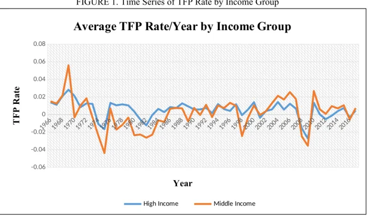
Figure 1 shows the average TFP rate each year for middle-income countries compared to high-income countries.3 On average, middle-income countries typically tend to have a lower TFP rate over the given time period. The middle-income trap is characterized by slowdowns in total factor productivity and Figure 1 shows that countries in the middle-income category, on average, are spending more years between 1965 and 2017 with a TFP rate closer to zero or negative.
FIGURE 1. Time Series of TFP Rate by Income Group
19661968197019721974197619781980198219841986198819901992199419961998200020022004200620082010201220142016
-0.06 -0.04 -0.02 0 0.02 0.04 0.06 0.08
Average TFP Rate/Year by Income Group
High Income Middle Income
Year
T
F
P
R
at
e
Table 2 shows summary statistics for the control variables used. They are life expectancy, age dependency ratio, trade openness, and a country dummy. Life expectancy is measured at birth. The age dependency ratio measures the ratio of dependents, people younger than 15 and older than 64, to the working-age population. Trade openness is measured as the sum of imports and exports divided by GDP. Data on those three controls come from the World Bank. I chose
3I did not include the low-income category because there are only four countries in it. Therefore,
these variables as controls because of their effect on driving productivity within the production function.
Life expectancy is used as a proxy for measuring the health of a country’s population. The healthiness of people, especially of working age, is important for productivity because unhealthy workers tend to be less efficient in the workplace, which in turn affects productivity (“WHO on Health and Economic Productivity,” 1999).
The age dependency ratio of a country can affect productivity via savings (Bloom & Williamson, 1997). A higher ratio leads to lower aggregate savings because there are more younger and/or older people in the population that are typically more of consumers rather than savers (Bloom & Williamson, 1997). Lower savings imply fewer funding opportunities for research and development, which affects technological innovation and in turn affects productivity (Bloom & Williamson, 1997).
Trade openness affects productivity because it is a mechanism that allows for the dissemination of knowledge and innovative technological process between countries (Chang et al. 2009).
The country dummy is 0 for the United States and 1 for all other countries. I included this dummy variable so TFP rates and the initial level of TFP for other countries are relative to a high-income country.
TABLE 2
Summary Statistics of Controls
Variable Mean SD Observations
Life Expectancy 68.580
8 10.437 3710
Age Dependency 65.908
Trade Openness 69.512
7 57.6653 3710
3.2 Explanatory Variables for Slowdowns
Table 3 shows the descriptive statistics of the key variables: slowdown and income inequality. Economic slowdown is a binary variable collected from the estimated residuals of running the regression in the first part of the empirical model. The residuals are defined as the actual rates of TFP growth minus the estimated rates of growth. A positive residual means that the country is growing faster than expected, while a negative residual means it is growing slower than expected. A positive residual is assigned a 0, while a negative residual is assigned a 1. This slowdown variable is divided into two separate variables. Slowdown2, defines slowdowns as a country that experiences at least two sustained periods of TFP growth that is below expected. This is represented by two negative residuals in a row. Slowdown3 more strictly defines
slowdowns as at least three sustained periods of TFP growth that is below expected, represented by at least three negative residuals in a row.
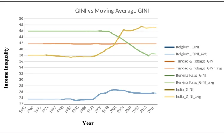
Income inequality is measured by an estimate of the GINI index of inequality in
inequality variable. The moving average technique takes the average of a subset of numbers to help capture the overall idea of the trend in the data set. Figure 2 shows that this data filling does not materially change the slope or dynamics of the data.4 Furthermore, the mean and standard deviation of the income inequality variable in both the original sample and the filled-in are very close.
TABLE 3
Summary Statistics of Key Variables Variable
Mean
Original Sample
SD Observations Mean
Filled-In Sample
SD Observations
Slowdown2 .391 .488 3640 .391 .488 3640
Slowdown3 .307 .461 3640 .307 .461 3640
Income Inequality 37.368 8.540 2799 37.555 8.528 3640
FIGURE 2. Plot of GINI w/ Missing Values vs. Filled-in
4This figure covers all income categories but consists of only four countries for adequate
1965 19681971 1974 1977 1980 1983 1986 1989 19921995 1998 2001 20042007 2010 2013 2016 22 24 26 28 30 32 34 36 38 40 42 44 46 48 50
GINI vs Moving Average GINI
Belgium_GINI
Belgium_GINI_avg
Trindad & Tobago_GINI
Trindad & Tobago_GINI_avg Burkina Faso_GINI Burkina Faso_GINI_avg India_GINI India_GINI_avg Year In co m e In eq u al it y
Table 4 shows the summary statistics for the controls used in this second part of the analysis. They are region, natural resource dependency, and export diversification. The number and choice of controls to include was limited due to the size of my sample and incomplete data from other databases and sources. Nevertheless, I chose these variables as controls because of their effect on technological change within a country and thus the rate of growth in total factor productivity. The variable region is used to control for the geographical location of where TFP slowdowns are occurring. The region variable is a dummy with countries located in South and Central America indicated by a 1 and countries in all other regions indicated by a 0.5 Natural resource dependency is measured by the amount of natural resource rents as a percent of GDP. This data comes from the World Bank. Export diversification measures whether the structure of exports by product of a country differs from the structure of exports of product by the world. The data for this index comes from the International Monetary Fund.
TABLE 4
Summary Statistics for Controls Variable
Mean
Original Sample
SD Observations Mean
Filled-In Sample
SD Observations
Natural Resource Dependency
3.977 5.718 3270 4.048 5.832 3640
Export Diversification 2.870 1.103 3162 2.804 1.136 3640
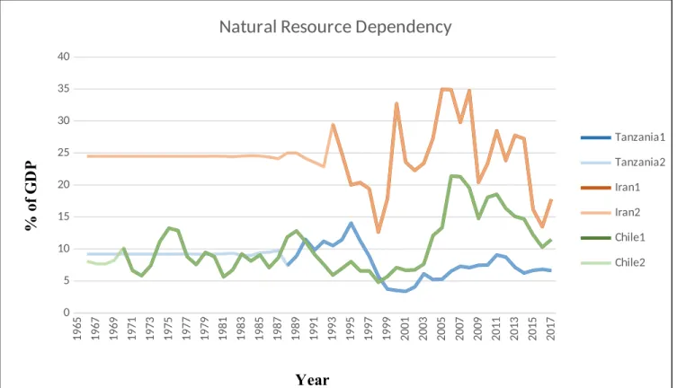
Once more, the data for my variables, natural resource dependency and export
diversification, is not complete. Therefore, I used the same technique as above with the income inequality variable to impute the missing observations in my data set. Figures 3 and 4 show that this technique also did not significantly change the slope of the original data for either variable.6 In both figures, a 1 represents the data sample for the country with missing values and the 2 denotes the data sample with filled-in values. Furthermore, the mean and standard deviation of the variables in both the original sample and the filled-in one are not that significantly different.
FIGURE 3. Plot of Variable w/ Missing Observations vs. Filled-in
1 9 65 1 9 67 1 9 69 1 9 71 1 9 73 1 9 75 1 9 7 7 1 9 7 9 1 9 8 1 1 9 8 3 1 9 8 5 1 9 8 7 1 9 8 9 1 9 9 1 1 9 9 3 1 9 9 5 1 9 9 7 1 9 9 9 2 0 0 1 2 0 0 3 2 0 0 5 2 0 07 2 0 09 2 0 11 2 0 13 2 0 15 2 0 17 0 5 10 15 20 25 30 35 40
Natural Resource Dependency
Tanzania1 Tanzania2 Iran1 Iran2 Chile1 Chile2 Year % o f G D P
196519671969197119731975197719791981198319851987198919911993199519971999200120032005200720092011201320152017
0 1 2 3 4 5 6 7
Export Diversification
Niger1
Niger2
Brazil1
Brazil2
Belgium1
Belgium2
Year
In
d
ex
L
ev
el
4 Empirical Model
4.1 Nonlinear Regression Model
This paper identifies and explains slowdowns in TFP in two parts. The first step is to identify total factor productivity slowdowns within the countries in the data set. To do this, the TFP rate is regressed on the initial TFP level and a set of controls, i.e.,
TFPGit=α+β1logTFPi t
0+β2Xit+β3Di+εit, (1)
where Xit are life expectancy, age dependency, and openness to trade for each country i in
time period t and Direpresents the country dummy.
income group- low, middle and high- to see if middle-income countries disproportionately experience more TFP slowdowns compared to both high and low income countries. The
hypothesis is, that it will show that convergence in TFP, or lack thereof due to slowdowns, plays a role in perpetuating the middle-income trap.
4.2 Probit Model
After identifying TFP slowdowns, the next step is to investigate the underlying reason for TFP slowdowns. In this paper, income inequality is the main determinant being considered. Using a random effects probit regression, each slowdown variable is regressed on income inequality and the group of controls. The equation follows:
SD2it=α+β1GINIit+β2Ri+β3Zit+εit (2)
SD3it=α+β1GINIit+β2Ri+β3Zit+εit, (3)
where SD2it and SD3it are the two definitions of slowdowns for each country i in time
period t. Ri is the dummy for region and Zit are natural resource dependency and export
diversification.
5 Results
5.1 Total Factor Productivity Slowdowns
The results from the first part of the study identifying slowdowns in total factor
productivity in countries from 1965-2017 are shown in Figure 1. Figure 1 shows the total number of slowdowns experienced by income group for both the loose and the stricter definition of a slowdown. From the graph, you can see that middle-income countries experience more
for slowdowns that are only two consecutive years, which is more likely to happen in countries of all income groups. After all, it could be the result of the macroeconomic environment in general. A down year in TFP rate can recover within the next period, so the stricter definition is more representative of TFP slowdowns disproportionally occurring in middle-income countries.
FIGURE 5. Frequency of Slowdowns by Income Group
High Middle Low
0 100 200 300 400 500 600 700 800
SD2
SD3
Income Group
#
of
s
lo
w
do
w
ns
5.2 Causes of TFP Slowdowns
the same and the magnitude does not change for all variables showing the same qualitative measure.7
The coefficients are listed for each of the variables with their standard errors in parentheses in Table 4. The signs on most of the variables are of predicted. For example, an increase in natural resource dependency will increase the probability of a slowdown, while an increase in export diversification will decrease the probability. Furthermore, being located in the South/Latin American region of the world increases a country’s chance of experiencing a
slowdown. However, the coefficient for the income inequality variable is not what I initially predicted. It has a negative sign, meaning that an increase in income inequality decreases the probability of a total factor productivity slowdown. The average marginal effect of a unit increase in income inequality is a .3 percentage point decrease in the probability of a slowdown occurring.
TABLE 5
Effect of Income Inequality on Slowdowns
(1) (2)
Income Inequality -.008*
(.005)
-.009* (.005)
Export Diversification -.031
(.034) (.039)-.047
NaturalResource .012**
(.006)
.026*** (.007)
Latin American .118
(.094) (.112).115
Constant .049
(.167)
-.198 (.194) *p<0.1, **p<0.05, ***p<.01
A reason for this could be that income inequality has different effects on countries at different income levels. Egawa (2013) demonstrates that income inequality rises when a country achieves middle-income status and that over the long term, its prevalence will continue to
7See Table 13 in appendix for results for data sample with missing values to see precision stays
hamper economic growth. He illustrates this using the Kuznets hypothesis. The Kuznets
hypothesis states that when a low income country grows rapidly it will typically lead to a worse income distribution in the initial state of development. This is predicted based off economic development involving a shift of labor and resources from the agriculture sector to industry and this urban, industrial sector has a higher income per capita compared to agriculture, causing a rise in the economy’s overall degree of inequality (Barro 2000). Then, as a country continues to develop, the size of the agricultural sector diminishes decreasing overall inequality as more of the poorer agricultural workers join the industrial sector and see a rise in real wages (Barro 2000). Furthermore, when a country reaches this middle-income status more egalitarian forces, such as increases in education and skilled labor, should improve the income distribution and help to further economic development to the next stages (Egawa, 2013). Therefore, the Kuznets hypothesis is that the relationship between a country’s income level and its degree of income inequality is shown as an inverted U-shape because inequality first increases and then later decreases during the process of economic development. Egawa (2013) shows that when a middle income country fails to narrow their income gap, then instead of continuing to experience economic growth, a decreasing growth rate could occur and cause the country to be stuck in the middle-income trap.
To see if income inequality effects on total factor productivity slowdowns is partially determined by a country’s income level, I first looked at the variance in between income groups to see if they were statistically different from one another. Table 6 shows the mean and standard deviation of the variable income inequality by income group. The mean level of income
economic development they are at. Then, as the Kuznets curve predicts, income inequality increases as countries attain middle income status, which is demonstrated by the middle-income group have the highest mean level of income inequality. Subsequently, as countries grow to the high-income level, income inequality will fall back down again, following that inverted U-shape.
TABLE 6
Summary Statistics of Income Inequality by Income Group
Income Group Mean SD
High 31.21
6 6.237
Middle 43.39
6 6.160
Low 41.66
9 3.015
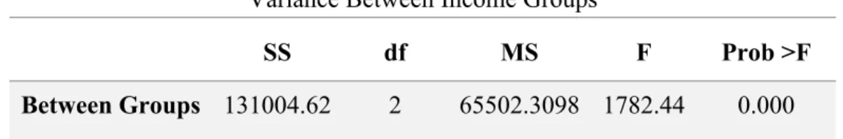
Table 7 shows the analysis of variance within the three income groups. The analysis shows that the mean level of income inequality between the three income groups is statistically significant at the 1% level.
TABLE 7
Variance Between Income Groups
SS df MS F Prob >F
Between Groups 131004.62 2 65502.3098 1782.44 0.000
Since there is evidence the level of income inequality is statistically different between the three income groups, I can look at how income inequality affects total factor productivity
rate in these countries. To examine this, I created two interaction variables to add to my probit regression. First, I created dummy variables for both the low and high income group. Then I interacted the GINI coefficient with both the low income and high-income dummy to generate the two interaction terms. I left out a variable for the middle-income because it acts as my reference group. The regression results after adding the two interaction variables are shown in Table 8.
TABLE 8
Effect of Income Inequality on Slowdowns w/ Added Interaction Variables
(1) (2)
Income Inequality -.003
(.006)
-.003 (.007)
Export Diversification -.021
(.034) -.021 (.039) NaturalResource .013 (.006) .027*** (.007)
Latin American .086
(.095)
.058 (.113)
GINI_LowIncome -.005
(.151) (.183)-.214
GINI_HighIncome .141 (.096) .113 (.113) Constant -.257 (.252) -.535 (.289) *p<0.1, **p<0.05, ***p<.01
inequality has on the two income groups demonstrates that the middle-income group is a transition point for the change in effects income inequality has, in that as low-income countries grow to the middle-income level their economy’s high level of unequal wealth distribution has negative effects on their TFP resulting in slowdowns and this high level of income inequality will continue to have negative effects even as the country moves to a higher income level. Therefore, income inequality seems to be an underlying factor of TFP slowdowns for middle-income countries, which potentially could be a reason that these countries get stuck in the middle-income trap. However, there is still no real significant difference in effects of income inequality on total factor productivity based on a country’s income level.
5.3 Robustness Check
TABLE 9
Other Determinants Effects on TFP Slowdowns
(1) (2)
Trade Openness -.0005
(.001) -.002*(.001)
Financial Openness .044**
(.022)
.070*** (.022)
Investment Share .672**
(.334)
.842** (.354)
Age Dependency Ratio .003
(.002)
.005** (.002)
Constant -.573
(.189)
-.908 (.204) *p<0.1, **p<0.05, ***p<.01
The signs on all the coefficients also match the results of the probit regressions from Aiyar et al. (2013). A higher age dependency ratio is associated with a higher probability of a slowdown because workers save, while dependents do not, therefore, effecting the national savings rate and decreasing the domestic resources available for productive investment. Increasing trade openness leads to a lower probability of a slowdown because of the opportunity for technological information sharing. The authors argue that financial liberalization may cause initial growth, but is hard for countries to sustain leading to reversals in the long run, which is why an increase in financial openness over the years may make countries more vulnerable to slowdowns. In addition, the authors again argue this “domestic overheating” that is associated with slowdowns is why an increase in an economy’s investment share might increase the probability of a slowdown.
TABLE 10
Income Inequality and Determinants Effects on Slowdowns
(1) (2)
Income Inequality -.004
(.005) (.006)-.003
Trade Openness -.0005
(.001)
-.002* (.001)
Financial Openness .0430**
(.021)
.070*** (.022)
Investment Share .625
(.340) .809**(.359)
Age Dependency Ratio .003
(.021)
.005** (.002)
Constant -.457
(.241) (.267)-.808
*p<0.1, **p<0.05, ***p<.01
6 Conclusion
This paper seeks to investigate the relationship between income inequality and total factor productivity slowdowns to determine if it is an underlying cause of countries getting stuck in the middle-income trap. Little empirical research has been done to assess income inequality’s role as a determining factor of slowdowns, specifically in total factor productivity. Examining this connection has important policy implications for middle-income countries who are searching for policy solutions to negative or stagnating growth they are experiencing. If income inequality is a determining factor, the special attention needs to be paid to policies that help to mitigate this such as a focus on investing in education to try and attain equal access, or redistributive policies, such as a progressive tax.
7 Appendix
TABLE 11
Income Classification of Countries in Sample
Low Middle High
Burkina Faso Argentina Australia
Niger Bolivia Austria
Mozambique Brazil Barbados
Tanzania Cameroon Belgium
China Canada
Columbia Chile
Costa Rica Cyprus
Cote d’Ivoire Denmark
Dominican Republic Finland
Ecuador France
Egypt Germany
Guatemala Greece
India Hong Kong
Indonesia Iceland
Iran Ireland
Jamaica Israel
Jordan Italy
Kenya Japan
Malaysia Luxembourg
Mexico Malta
Morocco Netherlands
Nigeria New Zealand
Peru Norway
Philippines Portugal
Romania Singapore
Senegal South Korea
South Africa Spain
Sri Lanka Sweden
Thailand Switzerland
Tunisia Trinidad & Tobago
Turkey United Kingdom
Venezuela United States
Zimbabwe Uruguay
TABLE 12
Region Classification of Countries in Sample
North America/Europe Asia/Pacific South & Latin America Middle East/Africa
Austria Australia Argentina Burkina Faso
Canada Hong Kong Bolivia Cote d’Ivoire
Cyprus India Brazil Egypt
Denmark Indonesia Chile Iran
Finland Japan Columbia Israel
France Malaysia Costa Rica Jordan
Germany New Zealand Dominican Republic Kenya
Greece Philippines Ecuador Morocco
Iceland Singapore Guatemala Mozambique
Ireland South Korea Jamaica Niger
Italy Sri Lanka Mexico Nigeria
Luxembourg Thailand Peru Senegal
Malta Trinidad & Tobago South Africa
Netherlands Uruguay Tanzania
Norway Venezuela Tunisia
Portugal Turkey Romania Zimbabwe Spain Sweden Switzerland United Kingdom United States TABLE 13
Effect of Income Inequality on Slowdowns w/ Missing Values Data Sample
(1) (2)
Income Inequality -.012*
(.006)
-.010 (.007) Export Diversification -.091*
(.050)
-.069 (.053)
NaturalResource .010
(.008) (.008).014*
Latin American .272**
References
Aiyar, M. S., Duval, M. R. A., Puy, M. D., Wu, M. Y., & Zhang, M. L. (2013). Growth Slowdowns and the Middle-Income Trap. International Monetary Fund.
Alesina, A., Ozler, S., Roubini, N., & Swagel, P. (1992). Political Instability and Economic Growth (Working Paper No. 4173). National Bureau of Economic Research.
https://doi.org/10.3386/w4173
Alvaredo, F., Chancel, L., Piketty, T., Saez, E., & Zucman, G. (2018). World Income Inequality Report.
Barro, R. J. (2000) ‘Inequality and Growth in a Panel of Countries’, Journal of Economic Growth vol. 5, no 1: 5-32.
Benhabib, J., & Spiegel, M. M. (1994). The role of human capital in economic development evidence from aggregate cross-country data. Journal of Monetary Economics, 34(2), 143–173. https://doi.org/10.1016/0304-3932(94)90047-7
Bloom, D. E., & Williamson, J. G. (1997). Demographic Transitions and Economic Miracles in Emerging Asia (Working Paper No. 6268). National Bureau of Economic Research. https://doi.org/10.3386/w6268
Chang, R., Kaltani, L., & Loayza, N.V. (2009). Openness can be good for growth: The role of policy complementarities. Journal of Development Economics, 90, pp.3-49.
Chinn, M., and Ito, H. (2006). What Matters for Financial Development? Capital, Controls, Institutions, and Interactions. Journal of Development Economics, 81(1), 163-192.
Eichengreen, B., Park, D., & Shin, K. (2013). Growth Slowdowns Redux: New Evidence on the Middle-Income Trap (Working Paper No. 18673). National Bureau of Economic Research. https://doi.org/10.3386/w18673
Felipe, J., Abdon, A., & Kumar, U. (2012). Tracking the Middle-Income Trap: What is it, Who is in it, and Why? (SSRN Scholarly Paper ID 2049330). Social Science Research Network. https://papers.ssrn.com/abstract=2049330
Feenstra, Robert C., Robert Inklaar, and Marcel P. Timmer. 2015. “The Next Generation of the Penn World Table.” American Economic Review 105 (10): 3150–82.
https://doi.org/10.1257/aer.20130954.
Gill, I.S., & Kharas, H. (2007). “An East Asian Renaissance: Ideas for Economic Growth.” World Bank, Washington, DC.
Gill, I. S., & Kharas, H. (2015). The Middle-Income Trap Turns Ten. The World Bank. https://doi.org/10.1596/1813-9450-7403
Im, F. G., & Rosenblatt, D. (2013). Middle-income traps: A conceptual and empirical survey (No. WPS6594; pp. 1–40). The World Bank. http://documents.worldbank.org/curated/en/ 969991468339571076/Middle-income-traps-a-conceptual-and-empirical-survey
International Monetary Fund. “Export Diversification.”
https://www.imf.org/external/np/res/dfidimf/diversification.htm
Krieger, T., & Meierrieks, D. (2016). Does Income Inequality Lead to Terrorism? (SSRN Scholarly Paper ID 2766910). Social Science Research Network. https://papers.ssrn.com/ abstract=2766910
Nel, P. (2003). Income Inequality, Economic Growth, and Political Instability in Sub-Saharan Africa. The Journal of Modern African Studies, 41(4), 611–639. JSTOR.
Odedokun, M. O., & Round, J. I. (2004). Determinants of Income Inequality and Its Effects on Economic Growth: Evidence from African Countries. African Development Review, 16(2), 287–327.
Ritzen, J., & Woolcock, M. (2000). SOCIAL COHESION, PUBLIC POLICY, AND ECONOMIC GROWTH: 33.
http://documents.worldbank.org/curated/en/914451468781802758/820140748_20040414
0033848/additional/28741.pdf
Solt, F. 2019. “Measuring Income Inequality Across Countries and Over Time: The Standardized World Income Inequality Database.” SWIID Version 8.1.
WHO on Health and Economic Producitivty. (1999). Population and Development Review, 25(2), 396-401. www.jstor.org/stable/172446.
World Bank. “Age Dependency Ratio (% of working-age population).” The World Bank Group.
https://data.worldbank.org/indicator/SP.POP.DPND
World Bank. “Life Expectancy at Birth, Total (years).” The World Bank Group.
https://data.worldbank.org/indicator/SP.DYN.LE00.IN
World Bank. “Total Natural Resources Rents (% of GDP).” The World Bank Group.