ENTRAINMENT DOMINATED EFFECTS IN THE LONG RESIDENCE TIMES OF SOLID SPHERES SETTLING IN SHARPLY STRATIFIED
MISCIBLE VISCOUS FLUIDS
Claudia Falcon
A dissertation submitted to the faculty at the University of North Carolina at Chapel Hill in partial fulfillment of the requirements for the degree of Doctor of Philosophy in the
Department of Mathematics.
Chapel Hill 2016
Approved by:
Roberto Camassa
Richard McLaughlin
David Adalsteinsson
Gregory Forest
c 2016 Claudia Falcon
ABSTRACT
Claudia Falcon: Entrainment dominated e↵ects in the long residence times of solid spheres settling in sharply stratified miscible viscous
fluids
(Under the direction of Roberto Camassa and Richard McLaughlin)
This dissertation presents results on the e↵ects of sharp density variations in the dynamics
of settling spheres in viscous – dominated regimes by a combination of experimental, analytical,
and numerical tools. Particles settling through naturally – stratified fluids, such as the ocean
and the atmosphere, a↵ect many aspects of life, from air quality and pollution clearing times
to the formation of thin aggregate layers in the upper ocean. In this thesis, we develop an
understanding of the dynamics that a↵ect these problems by studying the behavior of a
sphere falling under gravity through a two-layer fluid.
We have found that the sphere slows down dramatically as it passes through the density
transition. In this system, we demonstrate the importance of the entrained fluid to the
delayed settling of the particle due to its added buoyancy force. In particular, we compare
long residence times at the interface rivaling the ones observed for porous spheres and marine
snow – aggregates that occur naturally in the ocean – in similar configurations. We call these
cases the entrainment dominated regimes, where di↵usion of salt could play an active role
and it is therefore needed in the modeling.
The developed first principle model is a highly coupled system that captures the most
significant aspects of settling in a sharp two - layer fluid. We discuss previously implemented
approximations and new experimental regimes where the approximation is no longer valid.
The asymptotic approaches and exact solutions for the sphere exterior problem of the Stokes
equations will be compared in a parametric study of relevance for experiments. The region of
di↵usion in the entrainment dominated regimes will be discussed and explained.
The single particle theory further sheds light in the settling rates of marine aggregates
falling through sharp density transitions, and how this ultimately a↵ects marine carbon cycling.
In addition to solid spheres, we have examined porous, and drilled spheres , obtaining range
of parameters that enhance the residence time at the interface. We have also investigated
this phenomenon extensively through experiments by observing clouds of solid particles as
A mis padres
-El amor todo lo sufre, todo lo cree, todo lo espera,
todo lo soporta.
ACKNOWLEDGEMENTS
I would like to thank my committee members for their recommendations and my advisors
for the countless devoted hours of research, teaching, and mentorship. They have been
instrumental to my career since I joined their lab as an undergraduate. Roberto Camassa is
known for his unique guidance through difficult questions and making them seem easy through
simplified examples. I am thankful to Richard McLaughlin for his intuition, excitement for
interesting results, and challenging questions. Thank you for always pushing me to look
deeper after going over long pages of mathematics or sharing the results of an experiment.
Every meeting with them was a boost of energy to continue looking for solutions. Thank you
to both for your support through all these years.
I would also like to thank Joyce Lin. Her training introduced me to the field of fluid
dynamics and ultimately encouraged me to continue researching Mathematics at the graduate
level. I look up to her as a Mathematician and a friend and hope to continue collaborations
for years to come. A special mention must go to Kathryn Valchar for her immeasurable
hours of work and endless discussions that helped us improve our experimental techniques.
Her understanding of our goals made it easy to obtain good quality results. In addition,
thanks to Dylan Bruney, Sabina Iftikhar, and Gabriella Stein, for being the best team of
undergraduate researchers. Dylan’s innovative ideas and long hours in the lab until the
experiment was correctly completed, Sabina’s creativity and no-problem-is-too-big attitude,
and Gabi’s dedication to all aspects of the project helped us obtain the data shown in this
willing to advise on many numerical questions. Without his software and training, the analysis
would have been more difficult and less visually appealing .
A special mention must go to the UNC IME program coordinator, Kathy Wood, for
her hard work and support since my undergraduate years in AGEP. I am grateful for her
encouragement to pursuit challenging projects, her career development advice, and friendship.
Obvious acknowledgments go to the AGEP, Gates Millennium, NSF GRFP, and UNC
Graduate School Dissertation Completion fellowships. The National Science Foundation
has been a significant supporter of all the laboratory work. Specifically, credit is due to the
NSF-CMG and NSF RTG DMS-0502266 grants.
Last but not least, I am thankful for my family and friends for providing understanding
and many happy moments. I am thankful for my husband, who is a constant support when
deadlines require all my attention. His pride for my work and continuous encouragement is a
fuel like no other. There are no words to thank my parents for all their sacrifices. It gives me
great pleasure to talk about my work at a mathematical level with great thinkers like them.
My mom is my true confidant in moments of pressure and her words are always the ones I
need to hear. My dad was the first who taught me to explore creativity in a mathematical
way. I thank him for his willingness to always listen to my messy mathematical thoughts.
Thank you both for being my role models as mathematicians but also for making me want to
grow better everyday so that someday I get to be a teacher to my children the same way you
TABLE OF CONTENTS
Chapter 1. Introduction . . . 1
Chapter 2. First Principle Model . . . 4
2.1 Stokes flow in a cylinder . . . 7
2.2 Perturbation velocity . . . 12
2.3 Final Equations of motion . . . 14
Chapter 3. Stokes Solution Third Reflection . . . 16
3.1 Solution by Stream Function . . . 16
3.2 Second Reflection Approximation . . . 21
Chapter 4. The Oseen Tensor . . . 27
4.1 Definition of Perturbation Velocity . . . 27
4.2 Integrable Singularities . . . 28
4.3 Line of Removable Singularities . . . 30
4.4 Reducing volume integral to 2D integral . . . 32
Chapter 5. Experimental Work . . . 33
5.1 Methods . . . 33
5.2 Solid Sphere Experiments . . . 36
5.3 Porous Sphere Experiments . . . 41
6.2 Computation of w . . . 56
6.3 Interface Tracking Techniques and Validation . . . 57
Chapter 7. Theory Approximations . . . 60
7.1 Far Field Approximation . . . 60
7.2 Near Field Approximation . . . 65
7.3 Leaky Sphere Approximation . . . 66
7.4 Shell Model . . . 72
7.5 Perturbation Approach . . . 73
Chapter 8. Entrainment Dominated Regimes . . . 81
8.1 Comparison with Experiments . . . 82
8.2 Force Balance and the importance of Reflux . . . 84
8.3 Shell Depletion and Layer Thickness . . . 86
Chapter 9. Conclusions . . . 88
Appendix A. Oseen Integrals . . . 89
A.1 Integration procedure . . . 94
Appendix B. Holding Curve . . . 108
Appendix C. Flow Past a Stokeslet . . . 112
Appendix D. Di↵usion Coefficient in Corn Syrup . . . 115
D.1 Sodium Chloride NaCl . . . 115
D.2 Potassium Iodide KI . . . 116
Appendix E. Nomenclature . . . 118
LIST OF FIGURES
2.1 Schematic of the theoretical setup and notation. . . 5 2.2 Diagram of the Stokeslets located aty and y⇤. . . 13 3.1 Comparison of u(2) with its expansion as R/R0 ! 0 and Z/R0 ! 0,
eval-uating on the surface of the sphere r = pR2+Z2 = A, along ✓ = [0,⇡] discretized byn.Blue dots correspond to numerical integration and red dots to the approximation. Values are for A= 0.635cm, R0 = 5.4cm, V = 1. . . 26 5.1 Plot of water percentage vs. dynamic viscosity (P). This data aids the viscosity
matching process between the fluid layers of corn syrup. . . 35 5.2 Velocity profiles of sphere of radiusA= 0.641cmand density⇢s= 1.36712g/cm3
settling in a two-layer stratification with densities ⇢t = 1.34473g/cm3and ⇢b = 1.34767g/cm3 and average viscosity µ = 5.1595 Poise. The black line
represents the experiment tracking while, the dashed lines correspond to the theoretical terminal velocities and the vertical blue line shows the time at which the sphere is shown. . . 37 5.3 Velocity profiles of sphere of radiusA= 0.233cmand density ⇢s = 1.4g/cm3
settling in a two-layer stratification with densities ⇢t = 1.3616g/cm3and ⇢b = 1.36628g/cm3 and viscosities µt = 10.7307 Poise and µb = 11.0323
Poise. The black line represents the experiment tracking while, the dashed lines correspond to the theoretical terminal velocities. . . 38 5.4 Series of experiments from Stokes dominated regimes to Entrainment
domi-nated regimes. Experimentally measured velocity profiles of sphere of density
⇢s= 1.36712g/cm3 and radiusA = 0.641cm settling in a two-layer
stratifica-tion with similar top layer density and sequentially increasing bottom layer densities⇢b = 1.35425,1.36414,1.36623g/cm3 . . . 39
5.5 Velocity profiles of sphere of radiusA= 0.641cmand density⇢s= 1.36712g/cm3
settling in a two-layer stratification with densities ⇢t = 1.34647g/cm3and ⇢b = 1.35000g/cm3 and viscosities µt= 5.06980 Poise and µb = 5.27610 Poise.
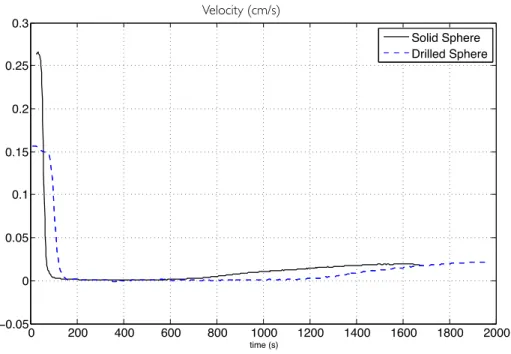
5.7 Velocity comparison between black solid line for the solid sphere and blue dashed line for the drilled sphere. . . 42 5.8 Velocity profile of drilled sphere with e↵ective density⇢sf = 1.36455 g/cm3 ,
computed terminal velocity for ⇢sf is shown in blue . . . 43
5.9 Velocity profile of drilled sphere initially with e↵ective density ⇢si = 1.36032
g/cm3 sinking in a homogenous surrounding fluid of density ⇢
f = 1.36364.
The drilled sphere begins to fall when its e↵ective density becomes larger than the ambient fluid due to di↵usion of salt. The theoretical terminal velocity for a solid sphere of density ⇢sf is shown in blue. . . 45
5.10 Velocity profile of drilled sphere with fluid rhof = 1.35883g/cm3 inside. Red
line indicates theoretical terminal velocity for a solid sphere of equivalent density⇢sf . . . 46
5.11 Velocity profile of drilled sphere initially with fluid ⇢i = 1.35050 g/cm3 inside,
computed terminal velocities for⇢si and⇢sf are shown in red and blue respectively 47
5.12 Velocity profile of drilled sphere with fluid rhof = 1.35976 g/cm3 inside . . . 48
5.13 Particle cloud settling in two-layer stratified fluid, the cloud sharpens as it reaches the interface. The stratification consists of a top layer with density
⇢t = 0.9987g/cm3 and a bottom layer of density ⇢b = 1.045g/cm3. The
particles are polystyrene beads of density⇢s = 1.05g/cm3 and average radius
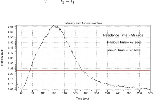
A= 0.02cm. . . 49 5.14 Concentration average around interface CI(t) versus time. The horizontal red
line denotes the 35% of the maximum value providing a residence time T = 99s. 51 5.15 Time-lapsed snapshots at (a) 2 s (b) 10 s (c) 15 s (d) 20 s of the particle
clouds settling in a two-layer of sharply stratified fluid, varying the size of the particles. The size of the beads increase from the first row to the last. . . 52 5.16 Residence time versus particle radius, the range of particle sizes inside a cloud
are denoted by the solid line, while the dots represent the mean size inside the cloud. . . 52 5.17 Residence time versus particle radius, read markings indicate porous particles
while black markings indicate solid beads. . . 53 5.18 Residence time as measured by CI (blue) and by CP (black) as we vary the
bottom layer density . . . 53 6.1 Diagram of domain of integration as determined by the entrainment and reflux
regions. The fluid domain ⌦f is shaded in blue and the sphere domain is
6.2 Disection of interface when (a) interface is below the sphere showing two regions of integration, (b) interface around the sphere, three regions of integration, and (c) interface above the sphere, four regions of integration. . . 56
6.3 Domain of integration and removable singularities. The blue dot represents the observation interfacial point and the red dashed line indicates where its corresponding line of removable singularities occur. These points only need to be dealt with when they get inside the blue shaded region, the fluid domain of integration. . . 57
6.4 Validation of interpolation, interface tracking and volume integrals by showing the point of zero Lagrangian displacement (top panels) and the normalized reflux volume (bottom panels) with potential flow for radius of sphereA= 1cm, interface initializedy0 = 10cm away from the sphere, and horizontal axial cut o↵ at (a)R0 = 40cm(b) R0 = 80cm (c) R0 = 320cm . The dashed lines represent the asymptotic value of each quantity. . . 58
6.5 Plots of interface advected with uniform velocity free space Stokes advection using (a) normal velocity and (b) full velocity . . . 59
7.1 Streamlines of the Oseen Green’s function far field approximation along the
x2 = 0 plane around a sphere of radiusA = 1 with one Stokeslet located at (a)
y= (0,0,2) , (b)y= (0.5,0, 1.1), (c) ring of points forces above and below 62
7.2 Non-dimensional numerically obtained velocity profiles using the far field approximation as the sphere density ⇢s ! ⇢b with ⇢t = 1.42760g/cm3 ,
⇢b = 1.43060g/cm3, and µ= 17 Pois. The red point represents the point that the interface goes into the sphere, deforming interface in a non-physical way and stopping the simulation . . . 63
7.3 Comparison of the streamlines along the x2 = 0 plane around a sphere of
radius A= 1 with one Stokeslet located aty = (0,0,2) of the Oseen Green’s function far field approximationWF F (left) and full kernel W(right) . . . . 63
7.4 Simulation of a sphere of density ⇢s= 1.4506g/cm3 settling in two layer fluid. Comparison of flow at the interfacial points. The blue arrows represent the stokes flow us while the red arrows indicate the perturbation flow using (a) the far field approximation wF F and (b) the full solutionw. . . 64
7.5 Far Field vs Full Theory in the Stokes dominated regime . . . 64
7.8 Shell model schematic showing the assumed spherical shell around the sphere. 72
7.9 Comparison of shell model with experiment and full theory. . . 73
7.10 Top layer and bottom layer domains . . . 78
7.11 Domain of integration for integrals It and Ib . . . 79
7.12 Domain of integration for Iw computed in code . . . 79
7.13 Domains of integration . . . 80
8.1 Plot of Archimedean buoyancy and density anomaly force as ⇢s!⇢b . . . . 81
8.2 (a) Interface at time t = 672 s, the last trusted time. (b)The sphere position. (c)The sphere velocity. The black solid lines are the experiment tracking, the blue dots are the theory prediction, and the black vertical lines indicate the last trusted time t=672 s. . . 83
8.3 Zoomed in plots of sphere position showing the code departure from experiment. 84 8.4 Experiment and theory comparison approaching the entrainment dominated regime. Left panel shows the model predicted interface and the right panel shows the experiment in black and the theory in blue. The experimental parameters are A= 0.641cm, ⇢s = 1.36712g/cm3, ⇢t = 1.34695g/cm3, ⇢b = 1.36178g/cm3, and µ= 4 Poise. . . . . 85
8.5 Experiment and theory comparison approaching the entrainment dominated regime. Left panel shows the model predicted interface and the right panel shows the experiment in black and the theory in blue. The experimental parameters are A= 0.641cm, ⇢s = 1.36712g/cm3, ⇢t = 1.34419g/cm3, ⇢b = 1.36639g/cm3, and µ= 5.75 Poise. . . . 85
8.6 Forces on the sphere for the Entrainment (w-dominated) regime showing the importance of the reflux portion to the motion of the sphere since the entrainment forceFE is bigger than the Archimedean forceFA for a portion of time. . . 86
8.7 Experimental picture showing the thin shell around the sphere for entrainment dominated regimes. . . 87
D.2 Picture of the di↵usion coefficient measurement set up inside the temperature bath . . . 116
CHAPTER 1
INTRODUCTION
Stratified environments frequently occur in nature. Examples include haloclines and
thermoclines in the ocean and atmosphere. These are often sharp density transitions formed
by density and temperature variations. Understanding how these sharp density di↵erences
a↵ect an immersed falling particle has applications from e↵ectively budgeting pollution in
the ocean to testing the efficiency of the ocean’s carbon pump. Thin layers of particulate
matter have been measured to accumulate at the density transitions found in coastal waters.
Marine snow particles are aggregates of organic and inorganic matter that are constantly
raining in the ocean, and are a major component of the ocean’s carbon cycle. When marine
snow accumulates at a density interface, the layers of aggregates become hotspots for bacteria
remineralization, preventing the particles from settling to the bottom of the ocean[31].
Understanding the residence time of these particles by studying the fluid mechanics behind
their settling in variable density fluids, can provide insight into the evolution of aggregates
and their fate as part of the carbon cycle.
There have been many studies of stratification and particle settling. Most of these
studies, however, involve homogenous or linear stratified fluid, and very few account for the
importance of entrainment in sharp density transitions. Some of the research investigating
sharply-stratified environments is restricted to immiscible fluids where surface tension is
dominant [3, 26]. Previous studies have also considered the settling of marine aggregates and
porous spheres in sharp stratifications [11, 31].
The behavior of a single sphere falling in sharp stratification has been been studied by
[1, 8, 9, 33], but many questions remain. Interesting phenomena have been discovered after
and sometimes even a directional (velocity) reversal, when falling under specific conditions
through a sharply stratified fluid [1]. As the sphere passes through the interface, the entrained
lower density fluid around the particle adds an extra buoyancy force that causes the delayed
settling. Solving this problem is a simplification of the settling of multiple aggregates but it
captures some of its most important dynamics.
The first–principle model that describes this behavior in viscous fluids is a highly coupled
system, derived by Camassa et. al. [8, 9]. Focusing on the low-Reynolds-number regime
simplifies the physics by making the fluid inertia negligible, which is reflected mathematically
by the linearization of the governing equations of motion. This makes them more accessible
to analysis and numerics. We use this model to study the dynamics of the long residence
times exhibited by solid spheres at density transition layers. In particular, we study the cases
with long residence times comparable to the ones observed for porous spheres and marine
aggregates in similar configurations. These cases fall into what we call the entrainment
dominated regime. This regime occurs when the di↵erence between the sphere density and
the bottom layer density (⇢s ⇢b) approaches the di↵erence between the bottom layer density
and the top layer density (⇢b ⇢t).When the residence times are comparable to di↵usion
time scales, salt di↵usion through the entrainment shell can play a significant role in the
sphere settling, making it important to understand its contribution in the modeling.
In order to compare the first-principle model solutions with the experimental data, we
need to numerically implement the final equations of motion, an integro-di↵erential equation
of the density of the fluid ⇢. The way in which we go about solving the resulting three
dimensional integral that defines the flow of the fluid determines the speed and accuracy
of the code. In this paper, we discuss previously implemented approximations and new
experimental parameters where these approximation are no longer valid. To remedy this, we
integrand- the Oseen tensor provided by [29]. The asymptotic approaches and exact solutions
for the sphere exterior problem of Stokes equations will be compared in a parametric study
of relevance for experiments. The region of validity for the approximations and the need to
implement matched asymptotic with the full solution will be discussed and explained.
Theoretically, there is much work to be done to understand the settling of marine
aggregates through sharp density transitions, and how this ultimately a↵ects marine carbon
cycling. To develop a mechanistic understanding of the behavior of these particles in the
ocean,we investigated this phenomenon in detail through experiments by observing clouds of
solid particles as they settle through a sharply stratified saltwater column. Chapter 5 describes
the experimental work and its Section 5.4 focuses on the multiple particle experiments in
sharply stratified fluids. The applications of our work can be instrumental for estimating
pollution-clearing times and the e↵ectiveness of the ocean as a pump in driving carbon excess.
Our study’s predictive tool gives us a better understanding on time scales and the attributes
of of delayed settling.
The set up of the single particle problem consists of a sphere of radius A settling under
gravity in an infinite cylinder of radiusR0 that contains a stable two-layer stratification of
miscible fluid, with top layer density ⇢t and bottom layer density of ⇢b. We are interested in
CHAPTER 2
FIRST PRINCIPLE MODEL
In this chapter, we set up the equations of motion for a solid sphere of radius A and
velocityV(t) = (0,0, V(t)) settling in sharp stratification and discuss the solutions as given by [9]. The Navier-Stokes equations for incompressible, Newtonian fluid of velocity v(x, t) and variable density⇢(x, t) and at an observation pointxin the fluid domain inside a cylinder of radius R0 are given by:
@⇢
@t +v·r⇢ = 0, r·v = 0, (2.1)
⇢
✓
@v
@t +v·rv
◆
= ⇢gˆ rp+µr2v, (2.2)
v = V(t) for|x Y3(t)|=A, (2.3) v = 0 for
q x2
1 +x22 =R0, 1< x3 <1, (2.4)
v ! 0 for |x3|! 1, (2.5)
where Y(t) is the position of the center of the sphere in the laboratory frame of reference, so that ˙Y3(t) =V(t), ˆg = (0,0, g) is the gravity acceleration vector with magnitudeg = 981cm/s2
.
By nondimensionalizing the equations of motion, important dimensionless parameters arise.
The Reynolds, Strouhal, and Froude numbers are defined as Re =AU/⌫, St=A/U T, and
x
3, Z
R 0
x
1, R
x 2 v(x, t)
A
V θ
Y
zˆ
Tuesday, June 14, 16Figure 2.1: Schematic of the theoretical setup and notation.
with the pressure scaled by µU/A. Our experiments are consistent with low Re number
regime making it possible to scale out the inertial terms, simplifying (2.6) to the Stokes
equation with variable density:
˜
r2v˜= ˜rp˜ Re
F r2 ⇢˜z.ˆ (2.7)
In dimensional form, the Equation (2.7), the incompressibility and boundary conditions,
for the Stoke’s approximation.
µr2v = rp ⇢g,ˆ (2.8)
r·v = 0, (2.9)
v = V(t) for|x Y3(t)|=A, (2.10)
v = 0 for
q x2
1+x22 =R0, 1< x3 <1, (2.11)
@⇢
@t +v·r⇢= 0. (2.13)
It is important to note that in equation (2.13) we have ignored di↵usion of salt, present
in the bottom layer fluid that serves as a stratifying agent . Some of our experiments –
the Entrainment regime experiments – slow down the settling rates and exhibit prolonged
residence times that are comparable with di↵usion time scales. By comparing those regimes
with this model, we can study the need for di↵usion to be included in the theory. In the
Stokes dominated regimes, we see the persistence of sharp interfaces between the upper and
lower fluids as well as along the entrainment around the sphere for the entire duration of
the experiment. These observations indicate that di↵usion is negligible in the Stokes regimes
while it may not be the case for the Entrainment Regimes. The di↵usivity of the salts used
in our fluids was measured and discussed in Appendix D. More evidence that no di↵usion
e↵ects are present in Stokes regime is given by the good agreement between experiments and
this non-di↵usive model. On the contrary, the Entrainment regimes show some discrepancy
when di↵usion time scales are of significance. These comparisons will be discussed in later
chapters.
The equation of motion for the sphere can be written as
ms dV(t)
dt =msˆg+
I
S ·
ˆ
n dS, (2.14)
where ms is the mass of the sphere, is the stress tensor, S is the surface of the sphere, and
ˆ
n is the outward normal unit vector to this surface.
The fluid flow can be written as
⇢0(x3) =⇢(x,0) while the second part, w(x, t), is what we call the perturbation velocity, as it has homogeneous boundary conditions and a forcing term⇢(x, t) ⇢0(x3). The equation of motion for the sphere becomes
ms dV(t)
dt =msgˆ+
I
S
u·ndSˆ +
I
S
w ·ˆndS, (2.16)
where u and w are the stress tensors for u and w, respectively. The latter stress tensor
w originates solely from the advection of the density field, and gives rise to an e↵ective
buoyancy-like force, which we refer to as the anomalous density force to distinguish it from
the usual Archimedean buoyancy.
2.1 Stokes flow in a cylinder
The equations of motion for the velocity component u(x, t) in equation (2.15), in the frame of reference of the sphere are
µr2u = rp
s ⇢0(x3+Y3(t))ˆg, (2.17)
r·u = 0, (2.18)
u = 0 for |x|=A, (2.19)
u = V(t) for
q x2
1+x22 =R0, 1< x3 <1 (2.20)
u ! V(t) for |x3|! 1. (2.21)
The solutions are given by the method of reflections used in [18], found by decomposing
the flow into a series
where
u(0) = V(t) (2.23)
u(1) =
8 > < > :
u(0) r=A 0 r !±1
(2.24)
u(2) =
8 > < > :
u(1) R =R 0
0 Z !±1
(2.25)
u(3) =
8 > < > :
u(2) r=A 0 r !±1
(2.26)
...
The flow is expressed by this infinite sum and can be truncated to the odd-labeled terms, making the flow satisfy boundary conditions on the sphere. On the other hand, when the
sum is truncated at the even-labeled terms the boundary conditions on the cylinder are satisfied. The first term u(0) is a constant flow (in space), whose inclusion changes the frame of reference from the lab frame to a frame of reference moving with the sphere. The second
term u(1) satisfies the boundary conditions using a sphere in Stokes flow in free space. [18] provide the full solution for the third term u(2), which cancels out the contribution of u(1) on the boundary of the cylinder. The magnitudes of u(0) and u(1) areO(1) and the sum of the two velocities satisfies the boundary conditions on the sphere. The error incurred on
the cylinder walls has magnitude O(A/R0). The next reflection u(2) has magnitude of order
O(A/R0), and the sum u(0)+u(1)+u(2) satisfies the boundary conditions on the cylinder so that this sum incurs an error on the sphere of order O(A/R0).
not computed explicitly, but we can expect that this pattern be repeated, so that the series
expansion u= (u(0)+u(1)) + (u(2)+u(3)) +. . .decreases by an order of magnitude in pairs, as indicated explicitly by the parenthetical grouping.
In the asymptotic expansion for u= u(0)+u(1)+u(2)+u(3). . ., as formulated in [18] in cylindrical coordinate (R,✓, Z) withr =pR2+Z2 is:
u(0)Z = V(t), (2.27)
u(0)R = 0, (2.28)
u(1)Z = V(t)
3A
4r
3AZ2 4r3
A3 4r3 +
3Z2A3
4r5 , (2.29)
u(1)R = V(t)
3ARZ
4r3 +
3A3RZ
4r5 , (2.30)
u(2)Z = 1
2⇡
Z 1
0 ˆ
uZ(R, ) cos( Z)d , (2.31)
u(2)R = 1
2⇡
Z 1
0 ˆ
uR(R, ) sin( Z)d , (2.32)
P(2)
µ =
1 2⇡
Z 1
0 ˆ
P(R, ) sin( Z)d , (2.33)
where
ˆ
uZ(R, ) =
R
2 (H( ) +G( ))I1( R) +H( )I0( R), (2.34) ˆ
uR(R, ) =
R
2 (H( ) +G( ))I0( R) G( )I1( R), (2.35) ˆ
and
H( ) = AV {3 (6 +A
2 2) (K
0( R0)I2( R0) +K1( R0)I1( R0))}
I0( R0)I2( R0) I1( R0)2
, (2.37)
G( ) = AV { 3 +A 2( R
0)2(K1( R0)I1( R0) +K2( R0)I0( R0))}
I0( R0)I2( R0) I1( R0)2
, (2.38)
with Ij and Kj are modified Bessel functions of the first and second kind.
For our purposes, we cannot truncate at the second reflection u(2), which is the last term of the series provided explicitly by [18]. Truncating at the second reflection would imply
satisfying boundary conditions on the wall but not on the sphere, therefore the interface
would pass through the sphere when u(3) is neglected, as this term is of the same order as u(2). In order to compute u(3), we must have u(2) on the surface of the sphere for boundary conditions. An expansion around small values R/R0 and Z/R0, can be made due to the
convergence properties of the infinity integral of the series expansion of the integrand (see
Section 3.2). Therefore, evaluated at the surface of the sphere, the second reflection u(2) , and thus the third reflection u(3) is
u(3)Z
r=A= u
(2)
Z
r=A = 2.10444 A R0
V 2.18004A 3
R3 0
V 0.140011 A
R3 0
R2V +. . .
u(3)R
r=A= u
(2)
R
r=A = 1.13669 A R3
0
R Z V +. . .
(2.39)
The solution of the third reflection problem using the expansion from Equation (2.39) for
u(3)R (R, Z) = 5A
8RV Z(( 1.13669) (0.140011)) (3R2 4Z2) 8R3
0r9
A6RV Z(( 1.13669) (23R2 12Z2) 6(2.18004)r2) 8R3
0r7
A6RV Z( 11(0.140011)R2+ 24(0.140011)Z2) 8R3
0r7
A4RV Z( 3( 2.10444)R2
0+ 3(2.18004)r2 2(0.140011)r2) 4R3
0r5 3A2( 2.10444)RV Z
4R0r3
(2.40)
u(3)Z (R, Z) = A
8V(( 1.13669) (0.140011)) (3R4 24R2Z2+ 8Z4) 8R3
0r9
A6V ( R2 Z2) ( 1.13669) (3R4 24R2Z2+ 8Z4) 8R3
0r9
A6V ((2.18004) ( 2R4+ 2R2Z2+ 4Z4) + (0.140011) (R4+ 20R2Z2 16Z4)) 8R3
0r9
A4V (( 2.10444)R2
0(R2 2Z2) + 3(2.18004) (R4+ 3R2Z2+ 2Z4)) 4R3
0r5
A4V ( 2(0.140011) (R4+ 3R2Z2+ 2Z4)) 4R3
0r5 3A2( 2.10444)V (R2+ 2Z2)
4R0r3
(2.41)
As mentioned in [9], the asymptotic properties of the reflection series as A/R0 !0 are not discussed by [18]. The asymptotic ordering of terms in equation (2.22) would fail near the
cylinder boundary, which would require techniques from matched asymptotics to address this
nonuniformity in a region near the cylinder’s boundary. By keeping the expansion up to the
third reflection, we no longer satisfy the boundary conditions on the cylinder exactly, but the
violation is consistent with the overall asymptotic error of the retained terms asA/R0 !0. All computations shown in this section use the above Happel and Byrne’s formulation.
used with variable density and time dependent sphere’s velocity to find the drag force due to
this flow,
I
S
s·ndSˆ = g
Z
⌦s
⇢0(x3+Y3(t))d⌦s 6⇡AµV(t)K, (2.42)
where ⌦s is the sphere domain and K = (1 2.10444(A/R0) + 2.08877(A/R0)3+...) 1 is
the drag coefficient.
2.2 Perturbation velocity
For the stratification-induced flow, we defineG(x, t) = (⇢(x, t) ⇢0(x3+Y3(t))) and write the governing equations in a moving frame of reference,
µr2w = rp
w G(x, t)ˆg, (2.43)
r·w = 0, (2.44)
w = 0 for |x|=A, (2.45)
w = 0 for
q x2
1+x22 =R0, 1< x3 <1 (2.46)
w ! 0 for|x3|! 1. (2.47)
Thus, the boundary conditions for w are homogeneous, and we can find an approximate solution for w(x, t) using the free space Green’s function due to [29]. This is the solution of the equations
µr2W(x,y) = rP(x,y) gˆ (x y), (2.48)
r·W = 0, (2.49)
W = 0 for |x|=A, (2.50)
for a Stokeslet of strength ˆg located at the point y outside a rigid sphere of radius A
surrounded by an infinite Stokes fluid. The resultant force on the sphere can be computed
using the Reciprocal Theorem [9].
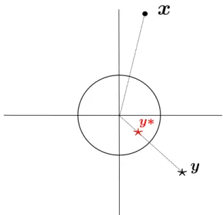
y
y
x
Figure 2.2: Diagram of the Stokeslets located at y and y⇤.
We look for an asymptotic expansion w = w(0) +w(1) +w(2) +w(3) +... for small (⇢(x, t) ⇢0). The first term of orderO(A/R0) can be written as the convolution
w(0)(x, t) =
Z
⌦f
G(y, t)W(x,y)d⌦f, (2.52)
p(0)w (x, t) =
Z
⌦f
G(y, t)P(x,y)d⌦f, (2.53)
where ⌦f is the fluid domain.
By interchanging the order of integration (which is allowed because of the convergence
becomes
I
S
(0)
w ijnjdS =
I
S
p(0)w ij +µ
@w(0)i @xj
+@w (0)
j @xi
!! njdS
=
Z
⌦f
G(y, t)
I
S
✓
P(x,y) ij +µ
✓
@Wi(x,y) @xj
+@Wj(x,y)
@xi
◆◆
njdS d⌦f
=
Z
⌦f
G(y, t)Aˆg 4
⇢
3 (r2+y2 3)
r3
A2(r2 3y2 3)
r5 d⌦f, (2.54)
where r=|y|.
Equations (2.52) and (2.54) determine the first order approximation to the fluid flow and
the resultant force on the sphere due to the density variation.
2.3 Final Equations of motion
Combining the results from Sections 2.1 and 2.2, we have the equation for the vertical
component of the velocity of the sphere and the advection of the fluid,
ms dV(t)
dt = msg g
Z
⌦s
⇢0d⌦s
6⇡AµV(t) 1 2.10444(A/R0) + 2.08877(A/R0)3+... 1
Z
⌦f
G(y, t)Agˆ 4
⇢
3 (r2+y2 3)
r3
A2(r2 3y2 3)
r5 d⌦f, (2.55)
@⇢
@t(x, t) + (u(x, t) +w(x, t))·r⇢(x, t) = 0. (2.56)
This can be further reduced when written in nondimensional form,
ReSt4⇡
3
⇢s ⇢ref
dV˜(t)
dt =
Re
F r2
✓ 4⇡ 3 ⇢s ⇢ref Z ˜ ⌦s ˜
⇢0d⌦˜s
◆
6⇡V˜(t) 1 2.10444(A/R0) + 2.08877(A/R0)3+... 1
which shows that the sphere’s acceleration term dV /dt can be scaled out. We are left with
˜
V(t) = Re
F r2 4⇡ 3 ⇢s ⇢ref Z ˜ ⌦s ˜
⇢0d⌦˜s+
Z
˜
⌦f
G(y, t) 4
⇢
3 (˜r2+ ˜y2 3) ˜
r3 +
(˜r2 3˜y2 3) ˜
r5 d⌦˜f
!
/(6⇡K),
(2.58)
St@⇢˜
@t˜(x, t) + (u˜(x, t) +w˜(x, t))·r˜⇢˜(x, t) = 0, (2.59)
where K = (1 2.10444(A/R0) + 2.08877(A/R0)3+...) 1.
In dimensional form, we have our final equations of motion for the sphere and fluid
velocities:
dY3
dt (t;⇢) = V(t;⇢) = (6⇡AµK)
1
✓
msg g
Z
⌦s
⇢0(x3+Y3(t;⇢))d⌦s+
+
Z
⌦f
G(y, t)Agˆ 4
⇢
3 (r2+y2 3)
r3 +
A2(r2 3y2 3)
r5 d⌦f
! ,
@⇢
@t(x, t) + (u(x, t;V) +w(x, t;⇢))·r⇢(x, t) = 0. (2.60)
The detailed formulations for the fluid velocitiy w can be found in Chapter 4. The formu-las (2.60) in addition to the equations (2.27)–(2.30) and (2.52) for the approximation to the
velocity field compose our final model for the settling of the sphere with the specified density
stratification.
Mathematically, this model is a coupled pair of integro-di↵erential equations in both
⇢(x, t) and Y3(t;⇢), where the speed of the sphere V(t) determinesu, and the density field
⇢(x, t) determines the domain of integration for w. The initial data completely determine the future evolution of the density field by advection through the fluid velocities, whose
combination satisfies the rigid boundary conditions (to within the accuracy of the analytic
approximations based on Stokes flow theory). The equations (2.60), show the highly coupled
system by emphasizing the dependence on ⇢ and V by writing them as arguments of the
CHAPTER 3
STOKES SOLUTION THIRD REFLECTION
3.1 Solution by Stream Function
The third reflection u(3) = ⇣u(3)
R ,0, u
(3)
Z
⌘
solves the Stokes equations with a prescribed
flow past the sphere. In cylindrical coordinates, the system of equations reads
µr2u(3) = rp(3) (3.1)
r·u(3) = 0 (3.2)
u(3)Z r=A
= u(2)Z r=A
= 2.10444A
R0
V 2.18004A 3
R3 0
V 0.140011A
R3 0
R2V (3.3)
u(3)R r=A
= u(2)R r=A
= 1.13669 A
R3 0
R Z V (3.4)
u(3) ! 0 as r ! 1. (3.5)
In spherical coordinates, axial symmetry acts the same as above andu(3) =⇣u(3)
r , u(3)✓ ,0
⌘
We
define the stream function to satisfy incompressibility. For the spherical coordinate system
(r,✓, ) , where✓ is the polar angle and the aximuzal angle, the stream function is defined
as
ur =
1
r2sin✓
@
@✓ (3.6)
u✓ = 1
rsin✓ @
The momentum equation and boundary conditions for becomes
✓
@2
@r2 +
sin✓ r2 @ @✓ ✓ 1 sin✓ @ @✓ ◆◆2
= 0, (3.8)
with boundary conditions
ur r=A
= 1
r2sin✓
@
@✓ r=A =B1cos✓+B2cos 3✓, (3.9)
u✓ r=A
= 1
rsin✓ @
@r r=A=B3sin✓+B4sin 3✓, (3.10)
where
B1 =
AV (2.10444R2
0 1.86086A2)
R3 0
(3.11)
B2 =
0.319175A3V
R3 0
(3.12)
B3 =
AV (2.3592A2 2.10444R2 0)
R3 0
(3.13)
B4 =
0.319175A3V
R3 0
(3.14)
and the behavior at infinity r! 1,
1
r2sin✓
@
@✓ r!1! 0 (3.15)
1
rsin✓ @
@r r!1! 0. (3.16)
The above restrictions leads us to find a solution of the form
From the boundary conditions, we obtain the following restrictions onf, g and h
4 (g(A) + 2h(A))
r2 = B1 (3.18)
8h(A)
r2 = B2 (3.19)
g(A) = f(A) h(A) (3.20) 2f(A)
r = B3 (3.21)
2h(A)
r = B4. (3.22)
The above together with the conditions at infinity, we get that the stream function is
(r,✓) = 20r3 1 Asin2(✓) 3A4(B2 4B4)
A2r2(5B1+ 6B2+ 10B3 14B4) + 5A2cos(2✓) A2(B2 4B4)
+ r2(4B
4 3B2) +r4( 5B1+ 3B2+ 10B3 2B4) ,
and the flow in spherical coordinate is,
ur =
A2V 4r5R3
0
cos(✓) A6(( 0.14001) (1.13669))
+ A4r2(3(1.13669) 2( 2.18001) + ( 0.14001))
+ A2 2(2.10444)r2R20 + 6( 2.18001)r4 (3.24)
4( 0.14001)r4 +A4 5A2 7r2 ((1.13669)
( 0.14001)) cos(2✓) + 6(2.10444)r4R20 ,
u✓ = A
2V
16r5R3 0
sin(✓) 9A6((1.13669) ( 0.14001)) A4r2((1.13669)
+ 4( 2.18001) 9( 0.14001))
4A2 (2.10444)r2R20 + 3( 2.18001)r4 2( 0.14001)r4 (3.25)
+ A4 15A2 7r2 ((1.13669)
( 0.14001)) cos(2✓) 12(2.10444)r4R2 0 .
Changing to cylindrical coordinates, we obtain the expression for the third reflection of
the stokes velocity.
u(3)R = 5A
8RV Z(( 1.13669) (0.140011)) (3R2 4Z2) 8R3
0r9
A6RV Z(( 1.13669) (23R2 12Z2) 6(2.18004)r2) 8R3
0r7
A6RV Z( 11(0.140011)R2+ 24(0.140011)Z2) 8R3
0r7
A4RV Z( 3( 2.10444)R2
0 + 3(2.18004)r2 2(0.140011)r2) 4R3
0r5 3A2( 2.10444)RV Z
4R0r3
,
u(3)Z = A
8V(( 1.13669) (0.140011)) (3R4 24R2Z2+ 8Z4) 8R3
0r9
A6V ( R2 Z2) ( 1.13669) (3R4 24R2Z2 + 8Z4) 8R3
0r9
A6V ((2.18004) ( 2R4+ 2R2Z2+ 4Z4) + (0.140011) (R4+ 20R2Z2 16Z4)) 8R3
0r9
A4V (( 2.10444)R2
0(R2 2Z2) + 3(2.18004) (R4+ 3R2Z2+ 2Z4)) 4R3
0r5
A4V ( 2(0.140011) (R4+ 3R2Z2 + 2Z4)) 4R3
0r5 3A2( 2.10444)V (R2 + 2Z2)
4R0r3
.
3.2 Second Reflection Approximation
Performing the change of variables ↵ = R0, the second reflection from Section (2.1),
u(2) =⇣u(2)
R ,0, u
(2)
Z
⌘
in cylindrical coordinates, is expressed as
u(2)R (R, Z) = 1 2⇡R0
Z 1
0 ˆ
uR(R/R0,↵) sin(↵Z/R0)d↵,
u(2)Z (R, Z) = 1 2⇡R0
Z 1
0 ˆ
uZ(R/R0,↵) cos(↵Z/R0)d↵,
(3.28)
where
ˆ
uR(R/R0,↵) =
↵R
2R0
⇣
H(↵) +G(↵)⌘I0
✓
↵R
R0
◆
G(↵)I1
✓ ↵ R R0 ◆ , (3.29) ˆ
uZ(R/R0,↵) =
↵R
2R0
⇣
H(↵) +G(↵)⌘I1
✓
↵R
R0
◆
+H(↵)I0
✓ ↵R R0 ◆ , (3.30) and
H(↵) =
AV n3 ⇣6 + AR22 0↵
2⌘ ⇣K
0(↵)I2(↵) +K1(↵)I1(↵)
⌘o
I0(↵)I2(↵) I1(↵)2
, (3.31)
G(↵) =
AV n 3 + AR22 0↵
2⇣K
1(↵)I1(↵) +K2(↵)I0(↵)
⌘o
I0(↵)I2(↵) I1(↵)2
, (3.32)
where Ij and Kj are modified Bessel functions of the first and second kind.
The integrals in equation (3.28) are not easily solved analytically, therefore to evaluate
the flow on the sphere we can perform an expansion far from the tank walls as R/R0 !0 and Z/R0 !0.
following series expansions which converge in the whole complex plane.
cos ( Z) = cos
✓ ↵Z R0 ◆ = 1 X n=0
( 1)n(↵Z)2n R2n
0 (2n)!
= 1 ↵ 2Z2
2R2 0
+. . . (3.33)
sin ( Z) = sin
✓ ↵Z R0 ◆ = 1 X n=0
( 1)n(↵Z)2n+1 R20n+1(2n+ 1)! =
↵Z
R0
+. . . (3.34)
I0( R) = I0
✓ ↵Z R0 ◆ = 1 X n=0
(1/4)n(↵R)2n n! (n+ 1)R2n
0
= 1 ↵ 2Z2
2R2 0
+. . . (3.35)
I1( R) = I1
✓
↵Z
R0
◆
= ↵R 2R0
1 X
n=0
(1/4)n(↵R)2n n! (n+ 2)R2n
0
= 1 ↵ 2Z2
2R2 0
+. . . (3.36)
The second reflection then becomes,
u(2)R = 1
2⇡R0
Z 1 0 d ↵ 2 R R0 ⇣
H(↵) +G(↵)⌘
1 X
n=0
(1/4)n(↵R)2n n! (n+ 1)R2n
0
(3.37)
G(↵)↵R 2R0
1 X
n=0
(1/4)n(↵R)2n n! (n+ 2)R2n
0
! 1
X
n=0
( 1)n(↵Z)2n+1
R20n+1(2n+ 1)!
! ,
u(2)Z = 1
2⇡R0
Z 1 0 d ↵ 2 R R0 ⇣
H(↵) +G(↵)⌘↵R 2R0
1 X
n=0
(1/4)n(↵R)2n n! (n+ 2)R2n
0
(3.38)
+ H(↵)
1 X
n=0
(1/4)n(↵R)2n n! (n+ 1)R2n
0
! 1
X
n=0
( 1)n(↵Z)2n R2n
0 (2n)!
! .
Here, we justify Happel and Byrne expansion as R/R0 ! 0 and Z/R0 ! 0 inside the infinite↵ integral. Using the asymptotic expansions as↵! 1 provided in [2] and the series representation, we show the convergence of the integrals of the partial sums due to their
exponentially decaying behavior as ↵! 1. Using,
Ij(↵) ⇠
↵!1
e↵
p 2⇡ R0
✓
1 4j 2 1 8 R0
+. . . ◆
(3.39)
Kj(↵) ⇠
↵!1 r
⇡
2↵e ↵
✓
1 + 4j 2 1
8↵ +. . .
◆
we get that,
H(↵) ⇠
↵!1
2⇡A3V
R2 0
↵3e 2↵. (3.41)
and,
H(↵) = ˆH(↵)2⇡A 3V
R2 0
↵3e 2↵ (3.42)
where ˆH(↵)!1 as ↵! 1. (3.43)
For the purpose of being brief, we focus on the last portion of the u(2)Z integral:
Z 1
0
F d↵=
Z 1
0
d↵H(↵)I0(↵R/R0) cos(↵Z/R0) (3.44)
F = H(↵)
1 X
n=0
(1/4)n(↵R)2n n! (n+ 1)R2n
0
!
cos (↵Z/R0). (3.45)
LetF =PFn, andFn given by:
Fn=H(↵)
(1/4)n(↵R)2n n!2R2n
0
cos(↵Z/R0) (3.46)
We know that,
Z 1
0
Fn d↵ C1
(1/4)n n!2
Z 1
0
↵2n+3e 2↵ d↵, (3.47)
Therefore solving the integral we get,
Z 1
0
Fn d↵C1
(1/4)n n!2
✓
(2n+ 3)! 22n+4
◆
taking the infinite sum 1 X n=0 Z 1 0
Fn d↵
1 X
n=0
C1
(1/4)n n!2
✓
2n+ 3 22n+4
◆
(3.49)
C1 22
9p3 (3.50)
< 1. (3.51)
And so, since
1 X
n=0
Z 1
0
Fn d↵<1 (3.52)
Then by the Lebesgue Dominated Theorem,
Z 1
0
F d↵=
1 X
n=0
Z 1
0
Fnd↵, (3.53)
and
Z 1
0
F d↵⇠
Z 1
0
N
X
n=0
Fnd↵. (3.54)
Therefore,
Z 1
0
d↵H(↵)I0(↵R/R0) cos(↵Z/R0) (3.55)
=
Z 1
0
d↵H(↵)
1 X
n=0
(1/4)n(↵R)2n n! (n+ 1)Rn
0
1 X
n=0
( 1)n(↵Z)2n R2n
0 (2n)!
(3.56)
⇠
Z 1
0
d↵H(↵) +
Z 1
0
d↵H(↵)↵ 2R2
4R2 0
+. . . (3.57)
(a)
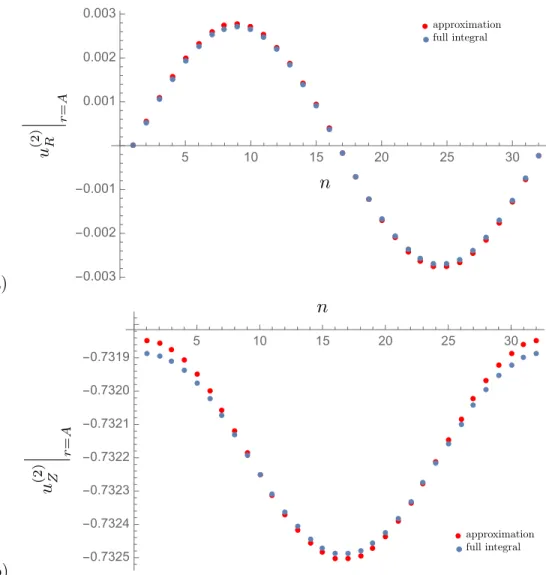
5 10 15 20 25 30
-0.003 -0.002 -0.001 0.001 0.002 0.003 n -0.7325 -0.7324 -0.7323 -0.7322 -0.7321 -0.7320 -0.7319 -0.7318 -0.7325 -0.7324 -0.7323 -0.7322 -0.7321 -0.7320 -0.7319 -0.7318 approximation full integral u (2) R r = A (b) -0.7325 -0.7324 -0.7323 -0.7322 -0.7321 -0.7320 -0.7319 -0.7318 -0.7324 -0.7323 -0.7322 -0.7321 -0.7320 -0.7319 -0.7318 approximation full integral
5 10 15 20 25 30
-0.7325 -0.7324 -0.7323 -0.7322 -0.7321 -0.7320 -0.7319 u (2) Z r = A n
Figure 3.1: Comparison of u(2) with its expansion as R/R0!0 and Z/R
0 !0, evaluating on the surface of the sphere r = pR2+Z2 = A, along ✓ = [0,⇡] discretized by n.Blue dots correspond to numerical integration and red dots to the approximation. Values are for
CHAPTER 4
THE OSEEN TENSOR
4.1 Definition of Perturbation Velocity
The perturbation velocity is written as a convolution with the Green’s function Wj(x,y),
wj(0)(x, t) =
Z
⌦f
✏G(y, t)Wj(x,y)d⌦f , (4.1)
where the Green’s function is written explicitly in terms of the Oseen tensor [29] Tjk as
Wj(x,y) =gTj3/8⇡µand
Tjk = jk
r +
(xj yj)(xk yk) r3
a |y|
jk r⇤
a3
|y|3
(xj yj⇤)(xk y⇤k) r⇤3
|y|2 a2
|y|
⇢y⇤
jyk⇤ a3r⇤
a |y|2r⇤3
⇥
yj⇤(xk yk⇤) +y⇤k(xj yj⇤)
⇤
+ 2y
⇤
jyk⇤ a3
y⇤
l(xl yl⇤) r⇤3
(|x|2 a2)@ k @xj
,
k = |
y|2 a2 2|y|3
✓
3yk ar⇤ +
a(xk yk⇤)
r⇤3 +
2yk
a y
⇤
j @ @xj
1
r⇤ +
3a |y⇤|
@ @y⇤
k
log |y
⇤|r⇤+x
jyj⇤ |y⇤|2 |x||y⇤|+xjyj⇤
◆ ,
where ais the radius of the sphere,y⇤ = a2
|y|2y,r =|y x|,r⇤ =|y⇤ x|, and the convention of sum over repeated indexes is used. Thus, the Green’s function can be viewed as resulting
from the superposition of appropriate singularities inside the radius-a sphere at the reflection
4.2 Integrable Singularities
The integrand Wj has a singularities at x=y coming from the terms
jk
r +
(xj yj)(xk yk) r3
a |y|
jk
r⇤ (4.2)
For simplicity, let us focus on the third component of the velocity W3, defining 12 terms
that add up to the total Green’s function vertical component. Each term is analyzed for
singularities separately.
W3 =
nX=12
n=1
In (4.3)
This first integrand term I1 is defined as
I1 = 1
r +
(x3 y3)2
r3 . (4.4)
The singularities of this term happen when
r =|x y|= 0 (4.5)
These singularities are integrable. In fact, in cylindrical coordinates
(4.6)
Z
⌦f
I1d⌦f
= Z ⌦f ✓ 1 r +
(x3 y3)2
r3
◆ d⌦f
=
Z
(⇢,⇣)
⇢d⇢d⇣
Z 2⇡
0
d✓⇣p 1
R2+⇢2 2R⇢cos( ✓) + (Z ⇣)2
+ (Z ⇣)
3
(R2+⇢2 2R⇢cos( ✓) + (Z ⇣)2)32
⌘
=
Z
(⇢,⇣)
⇢d⇢d⇣
4K⇣ R2 2⇢R+4R⇢2⇢+(⇣ Z)2
⌘
p
(⇢ R)2+ (⇣ Z)2 +
4(Z ⇣)2E⇣ 4R⇢ R2 2⇢R+⇢2+(⇣ Z)2
⌘
((⇢ R)2+ (⇣ Z)2)32
where K andE are elliptic integrals of the first and second kind respectively. To proof
integrability we multiply the integrand by an area element and bound it. If
lim
⇢!R ⇣!Z
⇣p
(⇢ R)2 + (⇣ Z)2⌘↵ I(⇢,⇣) M, (4.7)
then,
I(⇢,⇣) ⇣p M
(⇢ R)2+ (⇣ Z)2⌘↵ (4.8)
for ↵<2 because in a neighborhood D of (R, Z)
Z
D
M ⇣p
(⇢ R)2+ (⇣ Z)2⌘↵
d⇢d⇣ <1
)
Z
D
I(⇢,⇣) d⇢d⇣ <1
)
Z
D
I(⇢,⇣)d⇢d⇣ <1
(4.9)
The integrand has one singularity when R =⇢ andZ =⇣. Around this point (R, Z) =
I(⇢,⇣) = ⇢
✓
4K⇣ R2 2⇢R+4R⇢2+(⇢ ⇣ Z)2
⌘
p
(⇢ R)2+(⇣ Z)2 +
4(Z ⇣)2E⇣ 4R⇢
R2 2⇢R+⇢2+(⇣ Z)2
⌘
((⇢ R)2+(⇣ Z)2)32
◆
I ⇢
✓
4 p
(⇢ R)2+(⇣ Z)2 +
4(Z ⇣)2E⇣ 4R⇢
R2 2⇢R+⇢2+(⇣ Z)2
⌘
((⇢ R)2+(⇣ Z)2)32
◆
lim⇢!R ⇣!Z
⇣p
(⇢ R)2+ (⇣ Z)2⌘↵ ⇢
✓
4 p
(⇢ R)2+(⇣ Z)2 +
16R⇢(Z ⇣)2 ((⇢ R)2+(⇣ Z)2)2
◆
M
This remaining integrands with denominator r⇤ have no singularities becauser⇤ 6= 0 since
y⇤ is always located inside the sphere, exterior to the fluid domain.
4.3 Line of Removable Singularities
Before we integrate the Green’ s function over the fluid domain, it is convenient to combine
alike singularities and recognize cancelations. The line of removable singularities appears
when the observation pointxis co-linear with the evaluation pointyin the opposite direction. They come from the log term IL in the expression and cancel out leaving no problems in
the physical domain.
IL = I9+I10+I11+I12
IL =
|y⇤|⇣|x y1 ⇤|
(x3 y⇤3)2
|x y⇤|3
⌘
+ y3⇤(x3 y⇤3)
|y⇤||x y⇤| + 1 |y⇤|2+|y⇤||x y⇤|+x
1y1⇤+x2y2⇤+x3y3⇤
⇣
|y⇤|(x3 y⇤3)
|x y⇤| +y3⇤
⌘ ⇣
|y⇤|(x3 y⇤3)
|x y⇤| +
|x y⇤|y⇤
3
|y⇤| +x3 2y3⇤
⌘
( |y⇤|2+|y⇤||x y⇤|+x
1y1⇤+x2y2⇤+x3y3⇤) 2
x3y⇤3
|y⇤||x|+ 1
|y⇤||x|+x1y⇤1+x2y⇤2+x3y⇤3 +
⇣
|y⇤|x3
|x| +y3⇤
⌘ ⇣
|x|y⇤
3
|y⇤| +x3
⌘
As an example, lets take a closer look at the term I9,
I9 =
3A (x3 y3⇤) |y⇤|2(x3 y3⇤) +r⇤2y3⇤ r⇤2|y⇤|(|y⇤| r⇤)
r⇤3|y⇤|2(r⇤|y⇤| |y⇤|2+x
1y1⇤+x2y2⇤+x3y3⇤)
.
The singularities of this term I9 happen when its denominator vanishers at
r⇤|y⇤| |y⇤|2+x1y⇤1+x2y⇤2+x3y⇤3 = 0
|y⇤|
✓
r⇤ |y⇤|+x· y⇤
|y⇤| ◆
= 0
|y⇤|
✓
r⇤ |y⇤|+ (x y⇤ +y⇤)· y⇤
|y⇤| ◆
= 0
|y⇤|(r⇤+ (x y⇤)·n⇤) = 0
|x y⇤|+ (x y⇤)·n⇤ = 0
() x y⇤ =↵y⇤
|↵||y⇤|=↵y⇤· y⇤ |y⇤|
|↵|=↵
x=y⇤+↵·y⇤
↵<0
We can see the denominator of each term in IL vanishes along an entire line, and it is
not surprising that each term alone is divergent, since we know we need the addition of all
the log terms I9+I10+I11+I12 for the cancelation of singularities to occur.Plugging in the
log|y
⇤|r⇤+x
jy⇤j |y⇤|2
|x||y⇤|+xjyj⇤ xj=↵yj
(4.10)
= log|y
⇤||(↵ 1)y⇤|+↵y⇤
jyj⇤ |y⇤|2 |↵y⇤||y⇤|+↵y⇤
jy⇤j
(4.11)
= log|y⇤||(↵ 1)y⇤|+↵y⇤ ·y⇤ |y⇤| 2
|↵y⇤||y⇤|+↵y⇤·y⇤ (4.12) = log|↵ 1|+ (↵ 1)
|↵|+↵ (4.13)
which is independent of the variable of di↵erentiation y⇤3.
4.4 Reducing volume integral to 2D integral
The analytical integration in ✓ of each of the Ij terms is a long calculation (see Appendix
A). Most of the integrals can be computed by finding the integral of the form
F =
Z 2⇡
0
d✓
p
B+Ccos✓ =
4K
p
B+C (4.14)
and its derivatives with respect toB and C. In this expression, B and C are functions of the
CHAPTER 5
EXPERIMENTAL WORK
In this chapter we discuss experiments involving solid and porous spheres settling in the
low Reynolds regime, as well as particle clouds falling in homogenous and stratified finite
Reynolds fluids. The stratified density profiles include linear and sharp stratification. The set
up consists of miscible, often stably sharp stratifications of two layers and settling spheres
that are more dense than the ambient fluid densities.
We enhance the e↵ects of stratification and entrainment by studying a sphere in di↵erent
environments. We compare these results to that of a porous sphere, to make it a more similar
configuration to that of the ocean. Finally, experiments of multiple particles are performed
to show the extent of entrainment in the delayed settling of aggregates. All experiments shed
light to many issues of bio- and geo-physical applications. Similar to the higher Reynolds
number experiments in [1], we find that a single sphere exhibits a prolonged settling rate and
slows down substantially through a sharply stratified fluid. In addition, we find that there
are significant di↵erences between the Stokes dominated regime and the Entrainment regime,
where di↵usion of salt can play a role.
5.1 Methods
Clear, cylindrical plexiglass tanks with diameters ranging from 6.2 cm to 18.9 cm and
heights of either 31.8 cm or 52.1 cm are stratified with a top layer of lower density corn
syrup poured over a higher density (achieved by adding a chosen type of salt, often NaCl or
KI) corn syrup solution. We start with enough fluid for both layers that is mixed together
until homogenous. Then, we separate each layer and adjust with salt and water to attain
minimized by covering free surfaces with airtight membranes and thermal convection can be
controlled by a thermal bath.
The settling of multiple particles thorough density transitions is performed in a fish tank
with dimensions of 61.6 cm by 61.6 cm by 34.3 cm. Room temperature, DI water is mixed
with room-temperature salt water to create two layers of the desired densities. To obtain a
sharp stratification and minimize the density transition layer, we use a di↵user, composed of
a sponge surrounded by buoyant styrofoam. The bottom poured into the tank, we place the
di↵user carefully, and pour the top layer though the di↵user at a low speed. Conductivity
meters can measure the tank at discrete heights that helps us obtain a density profile. The
beads are then placed in a funnel closed with a plunger until release time to minimize initial
speed.
In the case of sharp stratifications, the method vary depending on the viscosity fluid. For
saltwater solutions, we use the same method as [1] - the bottom more dense layer is poured
first, then a floating di↵user is placed on the bottom layer and slowly pour the top layer less
dense fluid. The density profile is measured with an Orion conductivity probe. In the case of
corn syrup, we slowly pour the top layer sliding it down the inclined wall of the tank.
To obtain a linear stratification, we use the two-bucket method from [16], where the top
layer fluid from the first bucket is pumped into the mixing bucket at one half the flow rate as
the mixed fluid is pumped into the tank where the experiment is to be conducted.
5.1.1 Data Analysis
The data obtained from experiments is recorded by taking a video or pictures at uniform
intervals in time of the experiments. We then use DataTank - a graphical, object oriented
programming work environment- to track the position of the particle and its velocity is
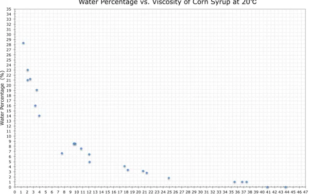
5.1.2 Matching viscosities
In order to compare our experiments with the theory, the viscosities between top and layer
fluid µt and µb must be matched within 2% of each other. The matching process requires
an extra level of careful measurements and adding water of to adjust while maintaining the
desired density. We have collected data to understand the e↵ect of water concentration in the
dynamic viscosity of corn syrup. Starting with pure corn syrup at 20oC of viscosity ⇡40P,
we add di↵erent amounts of water obtaining the plot in Figure 5.1.
0 1 2 3 4 5 6 7 8 9 10 11 12 13 14 15 16 17 18 19 20 21 22 23 24 25 26 27 28 29 30 31 32 33 34 35
0 1 2 3 4 5 6 7 8 9 10 11 12 13 14 15 16 17 18 19 20 21 22 23 24 25 26 27 28 29 30 31 32 33 34 35 36 37 38 39 40 41 42 43 44 45 46 47
W ate r Pe rce n ta ge (% )
Dynamic Viscosity (P)
Water Percentage vs. Viscosity of Corn Syrup at 20
Figure 5.1: Plot of water percentage vs. dynamic viscosity (P). This data aids the viscosity matching process between the fluid layers of corn syrup.
If the layers are di↵erent viscosities, we obtain di↵erent outcomes depending on which
viscosity is higher. We have performed experiments when the top layer viscosity µt is higher
than the bottom layer viscosity µb and vicerversa. So far, the observations show that if
µt> µb, then the sphere takes longer to achieve terminal velocity in the bottom layer. Further
5.2 Solid Sphere Experiments
In this section, we focus on the single solid sphere experiments settling in two-layer
stratifications. The solutions for a sphere settling in homogenous environment are well known.
Experimentally, we have homogenous runs in fluid of density equal to that of the bottom
layer density ⇢b as a bench mark to compare with the behavior of the sphere when settling in
the bottom layer of a two-layer stratified fluid. IN each layer, the sphere should approach the
theoretical terminal velocity.
Theoretically the terminal velocity in the bottom layer in the absence of entrainment is
given by :
Vb =
2K
9
gA2(⇢s ⇢b)
µb
(5.1)
where K = 2.10444(A/R0) 2.08877(A/R0)3 is the enhanced wall drag coefficient [18].
In two layers, the sphere slows down beyond its terminal velocity to the extra buoyancy
force provided by the entrainment fluid. In Figures (5.2) and (5.3), we show two Stokes
dominated experiments for di↵erent radius spheres. This e↵ect is magnified when the bottom
layer density approaches the density of the sphere, the sphere velocity approaches zero, and
the residence time increases. Because we are interested in testing the accuracy of the model
as we approach the entrainment regimes, we perform a series of experiments increasing the
bottom layer density. Examples of these experiments are portrayed in Figure (5.4). We note
that if viscosities are not very closely matched, the results would be not agree perfectly with
time: 95 s A = 0.641 cm, ρt = 1.34473, ρb = 1.34767, μ= 5.1595,
60 70 80 90 100 110 120 130 140 150 160
-5 0 5 10 15
time (s)
sp
h
e
re
p
o
si
ti
o
n
(cm)
60 70 80 90 100 110 120 130 140 150 160
0.10 0.15 0.20 0.25 0.30
time (s)
sp
h
e
re
ve
lo
ci
ty
(cm/
s)
Figure 5.2: Velocity profiles of sphere of radius A= 0.641cmand density ⇢s= 1.36712g/cm3