ELUCIDATION OF CHEMICAL REACTIONS BY TWO-DIMENSIONAL RESONANCE RAMAN SPECTROSCOPY
Brian Paul Molesky
A dissertation submitted to the faculty of the University of North Carolina at Chapel Hill in partial fulfillment of the requirements for the degree of Doctor of Philosophy in the Department
of Chemistry in the College of Arts and Sciences
Chapel Hill 2016
ABSTRACT
Brian Paul Molesky: Elucidation of Chemical Reactions by Two-Dimensional Resonance Raman Spectroscopy
(Under the direction of Andrew Moran)
It has been shown for many systems, including photosynthetic complexes, molecule-semiconductor interfaces, and bulk heterojunctions, that interaction between electronic and nuclear dynamics may heavily influence chemical mechanisms. Four-wave-mixing
spectroscopies (i.e. transient absorption, two-dimensional spectroscopy) provide some insight into such non-equilibrium processes but are limited by the single “population time” available in these types of experiments. In this dissertation, two-dimensional resonance Raman spectroscopy (2DRR) is developed to obtain new information regarding chemical reactions that possess time coincident electronic and nuclear evolution. These new insights can only be acquired through higher-order techniques possessing two “population times”. Specifically, the coherent reaction mechanism in triiodide photodissociation and structural heterogeneity in myoglobin are
investigated.
modes contributes to the signal. Under off-resonant conditions signal generation depends on much weaker effects.
Upon absorption of light ranging from ~250 to ~500 nm triiodide photodissociates into diiodide and radical iodine on the same time scale as the period of triiodide’s symmetric stretch, impulsively initiating coherence in the stretching coordinate of diiodide. In this dissertation, the sensitivity of 2DRR to coherent reaction mechanisms is shown by directly measuring, for the first time, how the nonequilibrium geometry of triiodide at the moment of photodissociation determines the stretching frequency of diiodide.
ACKNOWLEDGEMENTS
TABLE OF CONTENTS
LIST OF TABLES ... xiii
LIST OF FIGURES ...xiv
LIST OF ABBREVIATIONS AND SYMBOLS ... xxxv
CHAPTER 1: INTRODUCTION ...1
1.1. Uncovering Ultrafast Chemistry in Condensed Phases ...1
1.2. Development of Multidimensional Resonance Raman Spectroscopy ...2
1.3. Coherent Photodissociation of Triiodide ...5
1.4. Structural Heterogeneity and Vibrational Energy Exchange in Myoglobin ...8
1.5. Dissertation Contents ... 12
1.6. References ... 14
CHAPTER 2: SPECTROSCOPY AND DYNAMICS IN CONDENSED PHASES ... 24
2.1. Introduction ... 24
2.2. Time Dependent Perturbation Theory for the Density Operator ... 26
2.3. Obtaining the Line Broadening Function ... 30
2.4. Feynman Diagrams and Response Functions ... 36
2.5. Summary ... 44
2.6. References ... 46
CHAPTER 3: Methods of Femtosecond Pulse Generation and Relevant Ultrafast Techniques ... 48
3.1. Introduction ... 48
3.2. Spectral Broadening of Femtosecond Pulses Using Hollowcore Fibers... 49
3.4. Transient Absorption Spectroscopy ... 58
3.5. Transient Grating Spectroscopy ... 61
3.6. Six-Wave Mixing Spectrocopies ... 65
3.7. Femtosecond Stimulated Raman Spectroscopy by Six-Wave Mixing ... 70
3.8. Summary ... 74
3.9. References ... 75
CHAPTER 4: MULTIDIMENSIONAL RESONANCE RAMAN SPECTROSCOPY BY SIX-WAVE MIXING IN THE DEEP UV ... 80
4.1. Introduction ... 80
4.2. Experimental Methods ... 84
4.2.1. Third-Harmonic Generation via Filamentation in High-Pressure Ne ... 84
4.2.2 Six-Wave Mixing Interferometer ... 87
4.2.3. Sample Preparation ... 90
4.3. Model Calculations ... 91
4.3.1. Hamiltonian ... 91
4.3.2. Nonlinear Response Functions ... 92
4.3.3. Parameterization of Spectroscopic Model for Triiodide ... 98
4.3.4. Basis for Approximations in Response Function ... 99
4.4. Results and Discussion ... 101
4.4.1. Four-Wave Mixing Spectroscopy ... 102
4.4.2. Two-Dimensional Fourier Transform Resonance Raman Spectra ... 104
4.4.3. Analyzing Wavepacket Dynamics in Three Dimensions ... 110
4.5. Relative Magnitudes of Cascaded Third-Order and Direct Fifth-Order Signals in 2D Resonance Raman Spectroscopies... 116
4.5.1. Background ... 116
4.5.2. Model Calculations ... 118
4.5.3. Signatures of Direct and Cascaded Nonlinearities in Spectroscopic Line Shapes ... 124
4.5.4. Distinguishing Direct and Cascaded Nonlinearities Based on Signal Phases ... 126
4.5.6. Comment on the Relative Magnitudes of Third and Fifth-Order
Signals Fields ... 138
4.6. Conclusions ... 140
4.7. References ... 143
CHAPTER 5: ELUCIDATION OF REACTIVE WAVEPACKETS BY TWO-DIMENSIONAL RESONANCE RAMAN SPECTROSCOPY ... 150
5.1. Introduction ... 150
5.2. 2DRR Spectra Simulated for a Reactive Model System... 152
5.2.1. Model Hamiltonians ... 154
5.2.2. Response Functions ... 156
5.2.3 Calculated 2DRR Spectra ... 162
5.3. Experimental Methods ... 163
5.3.1. Conducting 2DRR Spectroscopy with a Five-Beam Geometry ... 164
5.3.2. Conducting 2DRR Spectroscopy with a Three-Beam Geometry ... 167
5.3.3. Sample Preparation and Handling ... 169
5.4. Experimental Results ... 169
5.4.1. Third-Order Stimulated Raman Response ... 169
5.4.2. 2DRR Response of the Diiodide Photoproduct ... 171
5.4.3. 2DRR Cross Peaks Between Triiodide and Diiodide ... 172
5.4.4. Summary of 2DRR Signal Components ... 175
5.5. Nonequilibrium Correlation Between Reactants and Products ... 177
5.6. Concluding Remarks ... 183
5.7. References ... 185
CHAPTER 6: FEMTOSECOND STIMULATED RAMAN SPECTROSCOPY BY SIX-WAVE MIXING ... 189
6.1. Introduction ... 189
6.2. Experimental Methods ... 193
6.2.1. Laser Pulse Generation ... 193
6.2.2. Laser Beam Geometries... 195
6.2.4. Sample Handling ... 198
6.3. Signal Processing ... 199
6.3.1. Algorithm ... 199
6.3.2. Adequate Suppression of the Broadband Response ... 204
6.3.3. Summary of Technical Issues Involved in Signal Processing ... 205
6.4. Experimental Results ... 207
6.4.1. Dependence of FSRS Signal on Incident Pulse Energies ... 207
6.4.2. Dependence of FSRS Signal on Sample Concentration ... 209
6.4.3. Relative Signs of Third- and Fifth-Order Signals ... 212
6.4.4. Dynamic Line Shapes of FSRS Signals Obtained by Six-Wave Mixing ... 215
6.5. Theoretical Analysis of Relative Magnitudes of Resonant FSRS Signals and Cascades ... 220
6.5.1. Background ... 220
6.5.2. Response Functions ... 221
6.5.3. Model Calculations ... 225
6.6. Concluding Remarks ... 229
6.7. References ... 231
CHAPTER 7: TWO-DIMENSIONAL RESONANCE RAMAN SPECTROSCOPY OF WATER- AND OXYGEN- LIGATED MYOGLOBIN... 236
7.1. Introduction ... 236
7.2. Experimental Methods ... 239
7.2.1. Sample Preparation ... 239
7.2.2. Spectroscopic Measurements ... 240
7.3. Simulations of 2DRR Spectra ... 243
7.3.1 Signatures of Inhomogeneous Broadening in 2DRR Spectra ... 244
7.3.2. Signatures of Anharmonicity in 2DRR Spectra ... 246
7.3.3. Predicted 2DRR Spectrum of Myoglobin ... 250
7.4. Results and Discussion ... 252
7.4.1. Isolation of 2DRR Signal Components ... 252
7.4.3. Computational Analysis of Line Broadening Mechanism ... 261
7.4.4. Implications for the Vibrational Cooling Mechanism ... 265
7.5. Concluding Remarks ... 266
7.6. References ... 268
CHAPTER 8: CONCLUDING REMARKS ... 274
8.1. Concluding Remarks ... 274
8.2. References ... 278
APPENDIX A: SUPPLEMENT TO “MULTIDIMENSIONAL RESONANCE RAMAN SPECTROSCOPY BY SIX-WAVE MIXING IN THE DEEP UV” ... 280
A.1. Auxiliary Response Functions ... 280
A.2. Anharmonic Excited State Potential Energy Surface ... 282
A.3. Modeling Concentration Dependence of Direct and Cascaded Responses ... 283
A.4. Third-Harmonic Generation via Filamentation in Neon at High Pressure... 285
A.5. Fifth-Order Cumulant Expansion ... 289
A.6. Reproducibility of Real and Imaginary Signal Components ... 294
A.7. Four-Wave Mixing Response in Region of Pulse Overlap ... 298
A.8. Derivation of Response Functions Used to Compute Ratio in Cascaded Third-Order and Direct Fifth-Order Signal Strengths ... 300
A.8.1. Third- and Fifth-Order Response Functions ... 300
A.8.2. Third and Fifth-Order Auxiliary Response Functions ... 306
A.8.3. Computing Relative Cascaded and Direct Signal Magnitudes ... 307
A.8.4. Magnitude of Prefactor ... 313
A.9. 2D Spectra for Sequential Cascades Simulated Using Measured Third-Order Signals ... 315
A.10. Tables of Phase-Matching Efficiencies for Three and Four-Beam Geometries ... 316
A.11. References ... 320
B.1. Vibrational Hamiltonian ... 322
B.2. Two-Dimensional Resonance Raman Signal Components ... 323
B.3. Derivation of Formula for the Direct Fifth-Order Signal Field ... 328
B.4. Dominance of the Direct 2DRR Response Over Third-Order Cascades ... 333
B.5. References... 336
APPENDIX C: SUPPLEMENT TO “FEMTOSECOND STIMULATED RAMAN SPECTROSCOPY BY SIX-WAVE MIXING” ... 338
C.1. Distinguishing the Broadband and FSRS Responses ... 338
C.2. Derivation of Formula for Direct Fifth-Order Signal Field ... 339
C.3. Derivation of Formula for Third-Order Cascaded Signal Field ... 350
C.3.1 Direct Coherent Stokes Raman Scattering (CSRS) Signal Field Obtained with the Phase Matching Condition k3 - k4 + k5 ... 351
C.3.2. Cascades with Intermediate Phase-Matching Conditions k1 – k2 + k5 and k3 - k4 + k5... 352
C.4. References... 361
APPENDIX D: SUPPLEMENT TO “TWO-DIMENSIONAL RESONANCE RAMAN SPECTROSCOPY OF WATER- AND OXYGEN- LIGATED MYOGLOBIN” ... 362
D.1. Response Functions... 362
D.2. Anharmonic Vibrational Hamiltonian... 365
D.3. Signatures of Anarhmonicity ... 366
D.4. Fluctuations in the Geometries of the Propionic Acid Side Chains... 369
LIST OF TABLES
Table 4.1. Parameters of Spectroscopic Model Based on Cumulant Expansion ... 101
Table 4.2. Dynamics in Correlation Spectra ... 116
Table 4.3. Parameters of Model Used to Compute Magnitudes of Direct Fifth-Order and Cascaded Third-Order Signals ... 129
Table 4.4. Calculated Wavevector Mismatches for Direct and Cascaded Nonlinearities in Geometry Shown in Figure 4.4 ... 139
Table 5.1. Parameters of Model Used to Compute 2DRR Spectra ... 161
Table 7.1. Parameters of Theoretical Model for System with Two Vibrational Modes ... 250
Table 7.2. Parameters of Model Based on Empirical Fit of Spontaneous Raman Signals ... 254
Table A.1. Calculated Wavevector Mismatches for Direct and Cascaded Nonlinearities in Geometry Shown in Figure 4.17a ... 318
Table A.2. Calculated Wavevector Mismatches for Direct and Cascaded Nonlinearities in Geometry Shown in Figure 4.17b ... 319
Table A.3. Calculated Wavevector Mismatches for Direct and Cascaded Nonlinearities in Geometry Shown in Figure 4.17c ... 320
Table A.4. Calculated Wavevector Mismatches for Direct and Cascaded Nonlinearities in the Three-Beam Pump-Repump-Probe Geometry (Data in Figure 4.19) ... 321
Table C.1. Parameters of Theoretical Model ... 357
Table C.2. Wavevector Mismatch in the Five-Beam Geometry ... 358
Table C.3. Wavevector Mismatch in the Four-Beam Geometry ... 359
LIST OF FIGURES
Figure 1.1. In a two-dimensional Raman experiment a pair of time-coincident laser pulses excites the sample before a delay period, τ1. Another pair of time-coincident pulses then reexcites the sample. After a second delay period, τ2, a final laser pulse induces signal emission. (a)Under off-resonant conditions, where the sample is transparent to the laser excitation and is thus promoted to virtual levels, selection rules dictate that harmonic modes cannot contribute to the signal intensity. Generation of the desired signal depends on weak effects like anharmonicity or nonlinear coordinate-dependence of the polarizability. This is the origin of the technical challenges experienced in multidimensional coherent Raman experiments conducted under off-resonant conditions. (b) Under resonant conditions, where the sample absorbs the laser light and is promoted to real excited states, both harmonic modes and anharmonic modes contribute to the signal generation mechanism, obviating the aforementioned challenges. ...4
Figure 1.2. Potential energy surface (PES) for the photodissociation of triiodide. 108,109 Here Rab and Rbc are the bond lengths between adjacent iodine atoms. A ground state wavepacket at equilibrium is promoted to the excited electronic state, where force is accumulated due to the steep gradient of the PES. A finite displacement in the asymmetric stretch induces photodissociation of triiodide into diiodide ions and iodine radicals. This entire process occurs in approximately 300 fs, the period of triiodide’s symmetric stretch. As such the reaction is impulsive and the wavepacket transitions from reactant to product without loss of coherence. 2DRR studies determine how the nonequilibrium geometry of triiodide at the time of photodissociation directly determines the distribution of vibrational quanta in
diiodide. ...6
Figure 1.3. (a) A single molecule of myoglobin in an aqueous bath. The heme group, colored in green, is tucked in the protein’s hydrophobic pocket except for the propionic acid side chains which extend into the surrounding environment and are hydrogen bound to water molecules. (b) The structure of the heme group possessed by myoglobin. The propionic acid side chains are circled in red. 2DRR studies suggest that structural heterogeneity of the propionic acid chains may play an important role in the fast rate of energy exchange between the heme and aqueous solvent. ...9
dimensions. Correlated 2DRR line shapes imply that geometric fluctuations are slow
compared to vibrational dephasing, indicating that the molecular structures involved possess geometric sub-ensembles at equilibrium (i.e. structural heterogeneity). (a)By integrating over dimension 1 a spectrum is obtained where the intensity in either (a) or (b), equivalently, is plotted against one frequency dimension. This is the type of spectrum gathered in 1D techniques (i.e. pump-probe). Information regarding inhomogeneous broadening, and thus structural heterogeneity, is not obtainable with 1D spectroscopies. ... 11
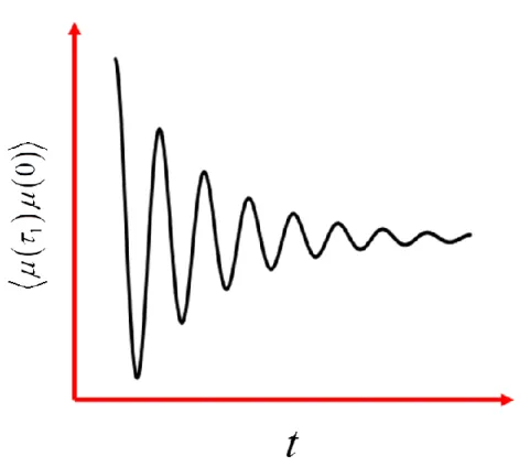
Figure 2.1. The line broadening function, g t
( )
, governs the damping of oscillations in the dipole operator correlation function due to random thermally driven collisions between the system and environment. After some time the oscillations dephase entirely as the systemloses memory of the state initially prepared by the perturbative electric field... 30
Figure 2.2. The energy gap between states of a two level system fluctuates about the mean due to random thermal motions of the environment. The fluctuations are characterized by their amplitude, ∆, and relaxation time, Λ−1 (see Equation 2.24). ... 31
Figure 2.3. In the homogenous limit of line broadening, absorption and fluorescence spectra possess Gaussian line shapes as described in Equations 2.28 and 2.29. ... 35
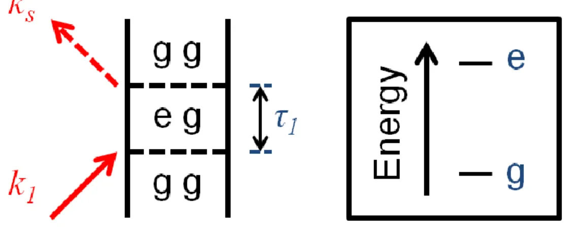
Figure 2.4. Feynman diagram for linear absorption of a two level system. Electric fields are denoted by their wavevectors. τ1 represents the time period of evolution between interaction with the incident field and signal emission. The term in the response function where k1 is
negative is irrelevant because the signal is measured in the direction of the incident field. ... 38
Figure 2.5. Convolution of a quasi monochromatic electric field with the term in the first order response function for linear absorption gives a Lorentzian line shape when a
homogeneous damping function is employed. A phase shift of −π2 is observed when the frequency of the incident field is equivalent to the electronic energy gap of the system.
Amplitude is quickly eliminated as the field is detuned from resonance... 39
Figure 2.6. Experimental geometry for the incident fields in a third order spectroscopy known as transient grating. k1 and k2 arrive simultaneously, there is a delay, and then k3 induces signal emission in the direction ks = − + +k1 k2 k3. In a traditional pump-probe experiment (transient absorption) the same phase matching condition applies; however the first two field matter interactions occur with a single field (the pump) such that k1=k2, and thus the signal is irradiated in the direction of the probe (ks =k3). ... 40
system considered here does not undergo population relaxation. Electric fields are denoted by their wavevectors and τ values represent periods of evolution between field matter interactions. Each diagram represents a term in the response function. GSB and ESE terms have a positive sign and correspond to a decrease in absorption relative to the ground state. ESA terms have a negative sign and correspond to an increase in absorption relative to the ground state. ... 41
Figure 2.8. Locations of the resonances measured by each of the six terms in the third order polarization given in Equation 2.37. The terms considered here measure the upper two quadrants. GSB and ESE (ESA) terms are positive (negative) two-dimensional Lorentzians that decay to 0 as the pump and/or probe are detuned from resonance. Terms in the
polarization possess significant amplitude only when both the pump and probe fields are
resonant with the corresponding electronic energy gaps of the system. ... 44
Figure 3.1. A Gaussian pulse propagating through a hollow-core fiber experiences self-phase modulation due to the intensity dependent refractive index of the gaseous medium. The frequency of the pulse experiences a red shift at the leading edge (i.e. t<0) and a blue shift at the trailing edge (i.e. t>0). At the peak (t=0), where the intensity possesses no
slope, the phase shift is 0 and there is no change in frequency. ... 51
Figure 3.2. The mounting system and air tight housing for a hollow-core fiber, specially designed to ensure perfect alignment to the path of the beam. The fiber is contained within a glass rod positioned within the central part of the housing. The rod is held in place by Swagelok Ultra-Torr fittings located where pairs of vacuum components are clamped together. The entire custom housing is highlighted in yellow, supported by four custom mounts. The image in red shows the fiber inside of the glass rod cradled by an Ultra-Torr fitting where the vacuum components have been disjoined to provide a better look. The gas inlet/outlet is circled in magenta. ... 53
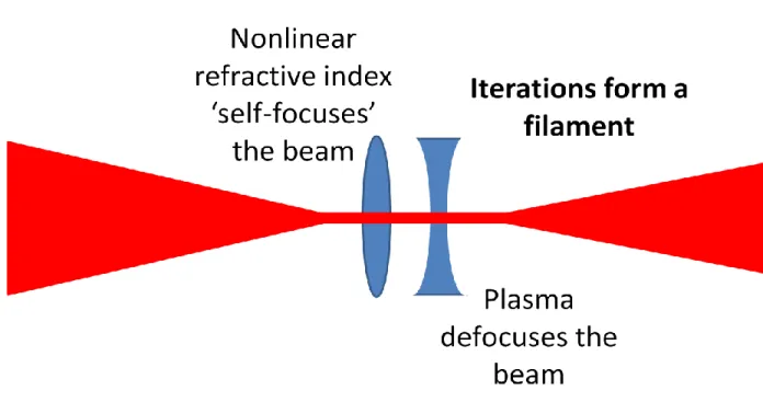
Figure 3.3. The process of filament generation. A high-energy laser beam is focused into a gas by a lens or mirror until the power density is great enough to cause Kerr effect induced self-focusing of the beam. The gaseous medium is ionized to form a plasma which defocuses the light. These processes iterate, forming a filament, until enough energy is lost through ionization of the gas to destabilize the balance between self-focusing from the Kerr-effect and defocusing from the plasma. Depending on the pulse duration and intensity as well as the type of gas and pressure, filaments can be as short as a centimeter or as long as meters. The filaments generated in this work are on the length scale of centimeters. ... 55
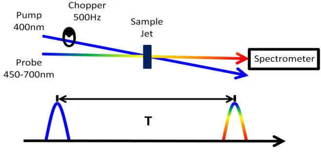
500Hz, half the rep rate of the laser, alternates between pump-on, pump-off conditions with each laser shot to measure the signal according to Equation 3.12. The signal is measured
over a delay range appropriate for the sample and dynamics of interest. ... 59
Figure 3.5. (a)The concept of grating formation in transient grating measurements. Two time-coincident noncollinear pump beams overlap in the sample interfering to form a population grating. After a delay the probe arrives and is scattered off the grating in the signal direction ks = − + +k1 k2 k3 where k1 and k2 are the pump beams and k3 is the probe. (b)An example population grating produced in a TG measurement viewed along the
propagation direction. The parameters used to calculate this grating correspond to
experimental conditions in Chapter 4. X and Y are dimensions in the laboratory frame. ... 62
Figure 3.6. The diffractive optic (DO) based interferometer used for TG measurements in this dissertation. Two beams enter the setup with an experimentally controlled delay between them. Both are focused onto the DO splitting each into its +1 and -1 diffraction orders. These four beams are incident on a spherical mirror which focuses them onto the sample. Beams 1-3 induce the polarization response and the signal is emitted collinearly with beam 4, an attenuated reference field for interferometric detection. A typical
interferogram is shown. ... 65
Figure 3.7. Experimental design of the pump-repump-probe experiments completed in this dissertation. A 400nm pump beam excites the sample from equilibrium. After a delay, τ1, another identical pump beam reexcites the system from a nonequilibrium state. There is another delay, τ2, and the probe arrives passing through the excited volume. Transmitted probe light is then dispersed by frequency on a suitable detector. Choppers in the paths of both pump beams spinning at 250Hz, a quarter of the laser’s rep rate, alternate between the four conditions needed to measure the signal according to Equation 3.16. Appropriate delay ranges are chosen based on the sample and dynamics of interest. ... 66
Figure 3.8. The diffractive optic (DO) based interferometer used for 4-beam six wave mixing experiments in Chapter 5. This setup operates much like the TG interferometer shown in Figure 3.6 but with a preliminary pump step (340nm pulse 1) such that there are two delay periods and four beams induce the polarization response of the sample. Again the signal is emitted collinearly with an attenuated reference field for interferometric detection. ... 68
reexciting the sample from a nonequilibrium state. Beam 5 induces signal emission
collinearly with an attenuated reference field, beam 6, for interferometric detection. ... 69
Figure 3.10. (a) An example population grating produced by the first pair of time coincident noncollinear pump beams in the 5-beam 6WM experiment. The number of fringes within the 120 micron FWHM spot size is reduced from 17 to 9 in comparison to TG experiments conducted under similar conditions. This reduction in fringe density originates in the lesser angular separation between pump beams. (b) The final 6WM grating from which the probe is scattered. The pattern is more complicated because two pairs of time coincident
noncollinear pump beams interfere to generate this grating. The parameters used to calculate both gratings correspond to experimental conditions in Chapter 4. Both gratings are viewed along the propagation direction. X and Y are dimensions in the laboratory frame. ... 70
Figure 3.11. (a) The interferometer used for FSRS by 6WM experiments in this dissertation. This design is much like the interferometer shown in Figure 3.9. However each of the three incoming beams is a different color. Therefore each exits the DO at a different angle preventing collinearity with a reference field. (b) The five-beam FSRS geometry. (c)The four-beam FSRS geometry. (d) The pulse arrival scheme. Actinic pump(s) arrive(s) first activating some electronic process. After a variable delay, τ1, the first Raman pump (beam 4) and the Stokes beam (beam 5) arrive. The window shown in (a) enforces another delay,
2
τ , and the final Raman pump (beam 3) is scattered off the FSRS grating. ... 72
Figure 3.12. (a) The static grating formed by the time coincident noncollinear actinic pump beams in the 5-beam geometry experiment. In the 4-beam experiment a singular actinic pump is used and this grating is not formed (b) In both the 4 and 5-beam experiments the Raman pump and Stokes beams create a dynamic population grating in the sample because the beams have different frequencies. The fringes move down to the right. (c)In the 5-beam experiment the gratings in (a)and (b) interfere forming a more complicated dynamic grating whose fringes move down to the left. In both the 4 and 5-beam experiments the final Raman pump is scattered off the respective dynamic grating, experiencing a ‘Doppler’ shift based on the fringe velocities. When that velocity matches a resonance frequency in the sample the signal is resonantly enhanced at the corresponding wavelength. ... 73
Figure 4.1. (a) The present experiment involves a sequence of five electronically resonant pulses and two experimentally controlled delay times. Coherent wavepacket motions are resolved in τ1 and τ2, whereas the signal frequency reflects the position and/or phase of the wavepacket. Fifth-order resonance Raman experiments can be used to investigate (b)line broadening mechanisms, (c) photochemical dynamics, and (d) shapes of potential energy
Figure 4.2. Setup used to generate third-harmonic laser pulses. Spectral widths of the 800-nm and 400-800-nm pulses are 350 cm-1 and 200 cm-1, respectively. Third-harmonic pulses with spectral widths greater than 300 cm-1 are obtained at 35 atm in neon gas. ... 85
Figure 4.3. (a) Pulse energy measured as a function of neon pressure. (b)
Intensity-normalized spectra of third-harmonic pulses measured as a function of neon pressure. (c) In neon, the spectral width measured for the full beam differs little from that of the central 25% (i.e. 25% of the intensity). Neon is superior to argon as a nonlinear medium in this respect (see Appendix A). ... 86
Figure 4.4. Diffractive optic-based interferometer used for six-wave mixing experiments. Each of the three incoming beams is split into 0, -1, and +1 diffraction orders with equal intensities (the diffraction orders are vertically displaced). Beams represented with open circles are blocked with a mask before the sample. The fifth-order signal is radiated in the direction k1− + − +k2 k3 k4 k5, and is collinear with the reference field (pulse 6) used for
interferometric signal detection after the sample. ... 88
Figure 4.5. Double-sided Feynman diagrams for the four dominant terms in the fifth-order response function. The indices g and e represent the ground state and the second-to-lowest energy excited state in I3-, respectively. Contributions from terms that evolve in excited state populations in t2 and t4 are negligible under our experimental conditions because of
ultrafast solvation, internal conversion, and photodissociation processes.46,49 ... 93
Figure 4.6. Measured and calculated absorbance spectra for I3- in ethanol are overlaid. The line shape of the second-to-lowest energy resonance is simulated using Equation 4.18. Parameters are given in Table 4.1. The lower energy resonance is approximated with a Gaussian function with a peak of 0.57, center of 27830 cm-1, and standard deviation of 1975 cm-1 in order to estimate its contribution to the low-energy side of the resonance of interest. ... 97
Figure 4.7. (a) Absolute value of the transient grating signal field for I3- in ethanol. The delay, τ , separates photo-excitation and detection. (b) Fourier transform of oscillations in the transient grating signals obtained at various detection wavenumbers. (c) Absolute value of stimulated Raman spectrum found by integrating over the detection wavenumber in panel (b). The symmetric stretch is located at 112 cm-1, whereas the lower energy resonance near 20 cm-1 corresponds to a (solute-solvent) intermolecular mode. ... 103
time-domain signals. A higher-quality Raman spectrum is obtained with the real signal
component. The non-oscillatory part of the signal has been subtracted from panels (a) and (b), so that the Raman response can be more clearly visualized. ... 107
Figure 4.9. 2D resonance Raman spectra computed with: (a) terms R1 and R3; (b) terms R2 and R4; (c) all terms, R1-R4. As in the experimental measurements, dominant resonances are found in the upper-right and lower-left quadrants. ... 109
Figure 4.10. (a) Correlation spectrum, S
(
ω ω2, t)
, measured at τ1=100 fs. (b) Isosurface of signal is drawn at 40% of the maximum intensity. (c) Mean detection frequency, ωt , andfit to Equation 4.20. (d) Mean vibrational frequency, ω2 , and fit to Equation 4.20. Noise associated with ωt and ω2 increases with τ1, because the signal magnitude decreases. Fitting parameters are given in Table 4.2. ... 112
Figure 4.11. (a) Correlation spectrum, S
(
ω ω2, t)
, calculated at τ1=100 fs. (b) Isosurface of signal is drawn at 60% of the maximum intensity. (c) Mean detection frequency, ωt , andfit to Equation 4.20. (d) Mean vibrational frequency, ω2 , and fit to Equation 4.20. Signals are calculated using the parameters given in Table 4.1. Fitting parameters are given in Table 4.2. ... 114
Figure 4.12. Dynamics in mean vibrational and emission frequencies, ω2 and ωt , adapted from the fits shown in Figures 4.10 and 4.11. The average values of the two
variables are shifted by small amounts between (a) experimental and (b) theory. The shapes of the spirals can still be directly compared because the magnitudes of the ranges are
identical in the two panels. It is predicted that anharmonicity, which is absent in the model,
causes the spiral to expand in the ω2 dimension. ... 115
Figure 4.13. Examples of Feynman diagrams associated with a direct fifth-order
nonlinearity, a sequential third-order cascade (k1− +k2 k3), and a parallel third-order cascade (k3− +k4 k5). The indices, g and e, represent electronic states, whereas dummy indices denote the vibrational energy levels of the ground (m,k,u) and excited electronic states (n,
l,v). In the cascaded third-order diagrams, interactions associated with blue arrows
correspond to emission and/or absorption of the field radiated at the intermediate step in the process. Direct fifth-order nonlinearities and third-order cascades involve three and four electronic coherences (shaded blue intervals) between the ground and excited states, respectively. As a consequence, contributions from third-order cascades decrease as the
Figure 4.14. Absolute values of the (a) direct fifth-order and (b) cascaded third-order signal magnitudes atω1=ω2=±112 cm-1 are shown for a dimensionless potential energy
displacement of 7.0, where an empirical anharmonic excited state potential energy surface is
employed (see Appendix A). The ratio, Ecas
(
ω ω1, 2)
/ E( )5(
ω ω1, 2)
, is computed using (blue) an empirical anharmonic model and (green) a harmonic model with equal ground and excited state frequencies (112 cm-1). The calculations suggest that third-order cascades in the Raman response are at least three orders-of-magnitude weaker than the direct fifth-order signal in I3- based on previous estimates for the displacement (7.0 and 8.8 for harmonic and anharmonic models, see Appendix A).48 The features at ω2=0 cm-1 (enclosed in boxes) in the cascaded signal spectrum represent imperfect subtraction of the non-oscillatorycomponent of the signal (this is not a vibrational resonance). ... 121
Figure 4.15. Parallel cascades that produce peaks at ω1=ω2=±112 cm-1 combine an oscillatory component of the response at one molecule (molecule A) with an incoherent component of the response at a second molecule (molecule B). The vibrational quantum number is changed by the first pulse-pair on molecule A, whereas a vibrational coherence is not produced in τ2 on molecule B (see Equation 4.24). The 2D line shape becomes
asymmetric (i.e. broader in ω2) if the magnitude of the polarization on molecule B relaxes (e.g. due to solvation) on the same time scale as vibrational dephasing. Parallel cascades at
1
ω =ω2=±112 cm-1 are much weaker than the direct fifth-order signal in I3-, because the oscillatory part of the third-order response is near 50% of the total third-order signal
magnitude. ... 123
Figure 4.16. Absolute values of two-dimensional Raman spectra (a) measured by six-wave mixing and (b) the parallel cascade computed using an experimental third-order transient
grating measurement. Slices of the two-dimensional Raman spectra are displayed at ω1=112 cm-1 (blue) and ω2=112 cm-1 (green) for the (c) experimental measurement and the (d) simulated parallel cascade. The line width of the parallel cascade is 30% larger in ω2 than it is in ω1 because of incoherent solvation dynamics in the ground electronic state. ... 126
Figure 4.17. (a)-(c)Three laser beam geometries are used to establish the relative phase-angles of third and fifth-order signals. Both signal fields are radiated in the direction,
3 4 5
direct fifth-order signals (obtained as the difference, beam 1,2 on – beam 1,2 off) at τ1=0.3 ps and τ2=0.3 ps. The interference fringes show that the third and fifth-order signal phases differ by approximately 180º (this behavior has been confirmed for delay times up to 3 ps). The measurement in panel (e) corresponds to geometry (a); the measurement in panel (f)
corresponds to geometry (b); the measurement in panel (g) corresponds to geometry (c). ... 128
Figure 4.18. (a) Absorptive parts of the wavelength-integrated third and fifth-order signal fields are measured using the geometry shown in Figure 4.17a. The delay axis, τ2,
corresponds to the delay between the pulse-pair 3,4 and pulse 5 (τ1=350 fs and τ2 is
scanned). (b) Absorptive parts of vibrational coherences are fit with sinusoidal functions to
quantify the phase difference. (c) The delay axis, τ1, is translated in the phase-difference associated with the absorptive components of third and (direct) fifth-order vibrational
coherences. The response is measured at a delay time predicted to yield an approximate 120° phase difference (at the dashed line). This control experiment suggests that the direct fifth-order Raman response is much larger than the cascaded nonlinearity... 132
Figure 4.19. (a) Pump-probe (ΔA) and (b) pump-repump-probe (ΔΔA) signals are measured simultaneously in a jet with a 300-μm path length using the three zeroeth-order laser beams in interferometer (signals are represented in mOD). The observation of signals with opposite signs in (a) and (b) indicates that the direct fifth-order response is greater than that associated with third-order cascades. The three-beam geometry is useful for establishing the intrinsic relative magnitudes of the direct and cascaded responses, because both nonlinearities are
well-phase matched. ... 135
Figure 4.20. Six-wave mixing signal intensities measured at (a) τ1=τ2=300 fs and (b) τ1 =300 fs, τ2=600 fs. Dependences of the direct (blue) and cascaded (red) signal intensities on the absorbance are simulated using the model described in Appendix A (the simulated
intensities are multiplied by constants in order to overlay them with the data). The
concentration dependences of the direct and cascaded processes differ, because the cascade is induced by the primary four-wave mixing response accumulated in the sample (see Appendix A). These data are consistent with dominance of the direct fifth-order signal field. ... 137
Figure 5.1. Linear absorbance spectra of triiodide and diiodide in ethanol. The absorbance spectrum of triiodide is directly measured, whereas that of diiodide is derived from Reference 35
Figure 5.2. Feynman diagrams associated with dominant 2DRR nonlinearities. Blue and red arrows represent pulses resonant with triiodide and diiodide, respectively. The indices r and
*
r represent the ground and excited electronic states of the triiodide reactant, whereas p
and p* correspond to the diiodide photoproduct. Vibrational levels associated with these
electronic states are specified by dummy indices (
m
,n
,j,k,l,u
,v
,w
). Each rowrepresents a different class of terms: (i) both dimensions correspond to triiodide in terms 1-4; (ii) both dimensions correspond to diiodide in terms 5-8; (iii) vibrational resonances of triiodide and diiodide appear in separate dimensions in terms 9-12. The intervals shaded in blue represent a non-radiative transfer of vibronic coherence from triiodide to diiodide. ... 158
Figure 5.3. Absolute values of 2DRR spectra computed using (a) the sum of terms 1-4 in Equation B.16, (b) the sum of terms 5-8 in Equation B.17, and (c) the sum of terms 9-12 in Equation B.18 (Equations B.16-B18 are in Appendix B). The frequency dimensions, ω1 and
2
ω , are conjugate to the delay times, τ1 and τ2 (see Figure 5.2). Signal components of the type shown in panel (a) are generally detected in one-color experiments. Two-color 2DRR approaches are used to detect nonlinearities that correspond to panels (b) and (c) in this work. The peaks displayed in Figure 5.3c are unique in that resonances of the reactant and product are found in ω1 and ω2, respectively. ... 163
Figure 5.4. (a) Diffractive optic-based interferometer used to detect signal components described by terms 5-8 in Figure 5.2. Each of the two 680 nm beams is split into -1 and +1 diffraction orders with equal intensities at the diffractive optic. The signal is collinear with the reference field (pulse 5) used for interferometric signal detection. (b) The 340 nm pulse induces photodissociation and vibrational coherence in the diiodide photoproduct during the delay, τ1. The time-coincident 680 nm pulses, 2 and 3, reinitiate the vibrational coherence in diiodide during the delay, τ2. ... 165
Figure 5.5. (a) Pump-repump-probe beam geometry used to detect signal components described by terms 9-12 in Figure 5.2. (b) The first 400 nm pulse promotes a stimulated Raman response in the ground electronic state of the triiodide reactant during the delay, τ1. The second pulse induces photodissociation of the non-equilibrium reactant, thereby giving rise to vibrational coherence in the diiodide photoproduct during the delay, τ2. Sensitivity to diiodide is enhanced by signal detection in the visible spectral range. ... 168
frequency reflects sensitivity to high-energy quantum states in the anharmonic potential of diiodide.19 ... 170
Figure 5.7. 2DRR signals associated with terms 5-8 are obtained using the two-color
approach described in Figure 5.4. (a) The total signal possesses both coherent and incoherent components. (b) The coherent (Raman) component of the signal is isolated by subtracting sums of two exponentials from the total signal presented in panel (a). (c) The
two-dimensional Fourier transformation of the signal in panel (b) in delay ranges, τ1 and τ2, between 0.15 and 2.0 ps reveals resonances in the upper right and lower left quadrants. This pattern of 2DRR resonances is consistent with calculations based on terms 5-8 (see Figure 5.3), which this experiment is designed to detect. ... 172
Figure 5.8. 2DRR data are obtained using the two-color approach described in Figure 5.5. Each column corresponds to a different detection wavenumber: 22,500 cm-1 (444 nm) in column 1; 21,000 cm-1 (476 nm) in column 2; 19,500 cm-1 (513 nm) in column 3; 18,000 cm -1
(555 nm) in column 4. (a)-(d) Total pump-repump-probe signal in mOD. (e)-(h) Coherent parts of the pump-repump-probe signals displayed in the first row. (i)-(l) 2DRR spectra are generated by Fourier transforming the signals shown in the second row in delay ranges, τ1 and τ2, between 0.15 and 2.0 ps. The data show that peaks in the upper left and lower right quadrants emerge as the detection wavenumber becomes off-resonant with triiodide. Signals acquired at detection wavenumbers above 21,000 cm-1 (476 nm) are dominated by stimulated Raman processes in the ground electronic state of triiodide (terms 1-4). In contrast, signals acquired at detection wavenumbers below 19,500 cm-1 (513 nm) are consistent with terms 9-12, where vibrational resonances in ω1 and ω2 correspond to triiodide and diiodide,
respectively. ... 174
Figure 5.9. Summary of 2DRR experiments conducted on triiodide: (a) the response of triiodide was detected in both dimensions in Reference 26; (b) the response of the diiodide photoproduct is detected in both dimensions (see Figure 5.7); (c) the response of triiodide and diiodide are detected in separate dimensions (see Figure 5.8). Blue and red laser pulses represent wavelengths that are electronically resonant with triiodide and diiodide,
respectively. ... 177
coherence frequency of diiodide is sensitive to vibrational motions of triiodide in the delay time, τ1. ... 178
Figure 5.11. The sequence of events associated with the 2DRR signals shown in Figure 5.10. Rab and Rbc denote the two bond lengths in triiodide. (a) The first pulse initiates a ground state wavepacket in the symmetric stretching coordinate. Force is accumulated when both bond lengths increase during the electronic coherence induced by the first laser pulse. (b) Wavepacket motion on the ground state potential energy surface is detected in the delay between the pump and repump laser pulses, τ1. (c) Photodissociation of triioide is initiated from a nonequilibrium geometry by the repump laser pulse. The Raman spectrum of
diiodide may then be detected by scanning the delay of a probe pulse, τ2. ... 180
Figure 5.12. Correlation between the vibrational wavenumber of the diiodide photoproduct and the pair of bond lengths in the triiodide reactant, Rab=Rbc, is illustrated by analyzing the dynamics in the mean vibrational coherence frequency, ω τvib
( )
1 , shown in Figure 5.10c. The delay time, τ1, is converted into the position of the wavepacket in the symmetricstretching coordinate using the model presented in Figure 5.11. Each revolution of the spiral corresponds to 300 fs. The wavepacket oscillates around the equilibrium bond length until vibrational dephasing is complete. The diagonal slant in the spiral suggests that a bond length displacement of 0.1 Å in triiodide induces a shift of 6.8 cm-1 in the vibrational
coherence frequency of diiodide. ... 182
Figure 6.1. (a) A five-beam FSRS geometry is used in this work to eliminate the portion of the background associated with residual Stokes light and third-order nonlinearities. The color code is as follows: the actinic pump is green, the Raman pump is blue, and the Stokes pulse is red. (b) Relaxation dynamics are probed in the delay between the actinic pump and Stokes pulses, τ1. The fixed time delay, τ2, is used to suppress a broadband pump-repump-probe response. ... 192
Figure 6.2. Spectra of the actinic pump (green), Raman pump (blue), and Stokes pulses (red) are overlaid on the linear absorbance spectrum of metmyoglobin (black) in aqueous
buffer solution at pH=7.0. ... 195
Figure 6.3. (a) Diffractive optic-based interferometer used for FSRS measurements. The transparent fused silica window delays pulse 3 by 290 fs with respect to pulse 4 (delay τ2 in Figure 6.1). (b) A five-beam geometry is used to detect the FSRS signal in the background-free direction, k1− + − +k2 k3 k4 k5. (c) The FSRS signal is also radiated in the direction,
1 2 3 4 5
3 4 5
k − +k k . In the four-beam geometry, the FSRS signal corresponds to the difference between signals measured with and without the actinic pump beam (beam 1,2). Beams represented with solid circles reach the sample, whereas those represented with open circles are blocked with a mask. The same color code is applied in all panels (Raman pump is blue, actinic pump is green, Stokes beam is red). ... 197
Figure 6.4. (a) This six-wave mixing signal for metMb is obtained in the five-beam FSRS geometry with τ2= 290 fs. The broadband baseline is subtracted to isolate the vibrational component of the response. (b) The baseline in panel (a) is obtained by inverse Fourier transforming the measured signal into the time domain, then filtering the broadband part of the response at 0 fs. (c) The baseline-subtracted signal is filtered at positive times after inverse Fourier transformation of the difference between the measured signal and the baseline shown in panel (a). The filter is displaced from the origin by 60 fs to eliminate the residual broadband response, which is dominant at earlier times. (d) The absolute value of the FSRS spectrum is obtained by Fourier transformation of the filtered signal in panel (c). .... 202
Figure 6.5. Molecular structure of iron protoporphyrin-IX. ... 203
Figure 6.6. This six-wave mixing signal for metMb is obtained in the five-beam FSRS geometry with τ2=420 fs. The panels (a)-(d) are defined in the same way as those in Figure 6.4. The vibrational frequencies obtained in this measurement differ by less than 10 cm-1 from those found in Figure 6.4. This difference is 5 times less than the bandwidth of the Raman pump pulse (i.e. intrinsic frequency resolution). The vibrational line widths are roughly 25% less than those shown in Figure 6.4. This decrease in the line width with
increasing delay, τ2, is consistent with the theory outlined in Section 6.5... 204
Figure 6.7. Signal intensities corresponding to the vibrational resonance at 1370 cm-1 are plotted versus incident pulse energies. In the first row, the signal, EFSRS
( )
ω EBB( )
ω , is plotted versus energies of the (a) actinic pump, (b) Raman pump, and (c) Stokes beams. Inthe second row, the signal, EFSRS
( )
ω , is plotted versus energies of the (d) actinic pump, (e) Raman pump, and (f) Stokes beams. Pulse energies associated with the actinic pump and Raman pump represent sums for the respective pairs of beams at the sample position (i.e. beams 1 and 2 or beams 3 and 4). The functional forms used to fit the data (red lines) are indicated in the respective panels. These data validate the signal processing algorithm described in Section 6.3 and confirm that saturation of the optical response is negligible in these ranges of the pulse energies. ... 209Figure 6.8. (a) FSRS signal intensities associated with the vibrational resonance at 1370 cm -1
functions, Idirect( )5
( )
C and Icascade( )
C , illustrate how the data compare to the concentration dependence predicted for (red) the direct fifth-order signal and (blue) third-order cascades.The functions, Idirect( )5
( )
C and Icascade( )
C , are multiplied by constants to overlay them with the measured signal intensities. (b) Dynamics in the peak intensity at 1370 cm-1 areexperimentally indistinguishable at various sample concentrations. (c) Signal intensities are overlaid at the highest and lowest concentrations to illustrate the range in the data quality. ... 212
Figure 6.9. (a) Signals acquired in the four-beam geometry at various delay times between the actinic pump and Stokes pulses, τ1. The signal atτ1=-0.5 ps is indistinguishable from the four-wave mixing signal measured with the actinic pump pulse blocked. (b) The fifth-order signal is obtained by computing differences between signals acquired with the actinic pump unblocked and blocked (i.e. pump on – pump off). Depletion of the ground state population with the actinic pump pulse is a signature that the direct fifth-order FSRS signal field is measured. In contrast, third-order cascades would induce an increase in the total signal intensity, because such nonlinearities are in-phase with the third-order response. (c) Oscillatory features associated with the vibrational resonances are phase-shifted by
approximately 180º in third- and fifth-order measurements (these are magnified views of the data in panels (a) and (b)). ... 214
Figure 6.10. (a) Contour plot of the signal field magnitude, EFSRS , obtained for metMb in the five-beam geometry. (b) Temporal decay profiles for vibrational resonances detected in the FSRS response. (c) Distributions of relaxation times for various resonances are obtained using the maximum entropy method. (d)-(f) FSRS signal field magnitudes are overlaid with fits conducted using the maximum entropy method. ... 217
Figure 6.11. Laser beam geometries used to acquire (a) stimulated Raman and (b) transient grating signals shown in (c) and (d), respectively. Beams represented with solid circles reach the sample, whereas those represented with open circles are blocked with a mask. (e) The two four-wave mixing signals are combined to simulate the cascaded response. (f) Unlike the FSRS signals plotted in Figure 6.10, all vibrational resonances decay with
indistinguishable temporal profiles in the simulated cascade. Signal magnitudes for the 670 and 1370-cm-1 vibrational resonances are shown as examples. ... 219
Figure 6.12. Double-sided Feynman diagrams associated with four classes of terms in the FSRS response function. The terms are classified according to whether or not they evolve in ground or excited state populations during the delay times, τ1 and τ2. The laser pulses associated with each field-matter interaction are indicated in the figure in the same
Figure 6.13. Feynman diagrams associated with the nonlinearities on the two molecules involved in third-order cascades with intermediate phase-matching conditions (a) k1− +k2 k5 and (b) k3− +k4 k5. Field-matter interactions are color-coded as follows: actinic pump is green; Raman pump is blue; Stokes is red; cascaded signal field is red; the field radiated at the intermediate step in the cascade is purple. ... 224
Figure 6.14. Absolute values of signal spectra computed using the models presented in Sections C.2 and C.3 in Appendix C and the parameters in Tables C.1 and C.2. The system possesses a single 1370-cm-1 harmonic mode with a displacement of 0.35 (a reasonable estimate for metMb).42 The frequency of the actinic pump pulse is set equal to the electronic resonance frequency, ωAP =ωeg. This calculation assumes that the five-beam geometry is employed (cascades are 4 times weaker in the four-beam geometry). ... 227
Figure 6.15. (a) The ratio, Ecas(ωt ) / Edirect( )5 (ωt ), is computed for a system with a single harmonic mode under electronically resonant conditions,ωAP =ωeg. The ratio is computed at the value of the Raman Shift equal to the mode frequency (i.e. at the peak of the vibrational
resonance). (b) The ratio, Ecas(ωt ) / Edirect( )5 (ωt ), is computed for a 670- cm -1
mode at various
dimensionless displacements and detuning factors, ωAP−ωeg. (c) The ratio, ( )5
( ) / ( )
cas t direct t
E ω E ω , is computed for a 1370-cm-1 mode at various dimensionless mode displacements and detuning factors, ωAP−ωeg. Boxes are drawn in the regions of the plots relevant to myoglobin in panels (b) and (c). ... 228
Figure 7.1. (a) A four-beam FSRS geometry is used in this work to eliminate the portion of the background associated with residual Stokes light and a pump-probe response. The color code is as follows: the actinic pump is green, the Raman pump is blue, and the Stokes pulse is red. (b) Vibrational coherences in τ1 are resolved by numerically Fourier transforming the signal with respect to the delay time. Time-coincident Raman pump and Stokes pulses then initiate a second set of vibrational coherences, which are resolved by dispersing the signal pulse on an array detector. The fixed time delay, τ2, is used to suppress the broadband
pump-repump-probe response of the solution. ... 238
Figure 7.2. Laser spectra are overlaid on the linear absorbance spectra of (a) metMb and (b) MbO2 in aqueous buffer solution at pH=7.0... 242
1 2 3 4 5
k − + − +k k k k ; the wavevectors k1 and k2 cancel each other. The 2DRR signal is obtained by measuring differences with and without the actinic pump (beam 1,2). Beams represented with solid circles reach the sample, whereas those represented with open circles are blocked with a mask. ... 243
Figure 7.4. 2DRR spectra computed for a pair of harmonic oscillators with inhomogeneous line broadening. The spectra are computed by combining Equations 7.1 and D.20 in
Appendix D with the parameters given in Table 7.1. The correlation parameter,ρ, is set equal to (a) -0.75, (b) 0.0, and (c) 0.75. The diagonal peaks always exhibit correlated line shapes, whereas the orientations and intensities of the off-diagonal peaks depend on the
correlation parameter, ρ. ... 247
Figure 7.5. 2DRR spectra computed with the anharmonic vibrational Hamiltonian described in Appendix D and the parameters in Table 7.1. The diagonal cubic expansion coefficients are set equal to -5 (first row), 0 (second row), and 5 cm-1 (third row). The off-diagonal expansion coefficients are set equal to -5 (first column), 0 (second column), and 5 cm-1 (third column). The response of a harmonic system is shown in panel (e). These calculations suggest that anharmonic coupling promotes intensity borrowing effects via the
transformation of Franck-Condon overlap integrals from the harmonic to anharmonic basis set (see Equation D.23 in Appendix D). For many of the parameter sets, anharmonicity causes the intensity of the cross peak above the diagonal to increase relative to that of the
cross peak below the diagonal. This effect is most pronounced in the left column. ... 249
Figure 7.6. 2DRR spectrum of myoglobin computed using parameters obtained by fitting spontaneous resonance Raman excitation profiles.67 The spectrum is dominated by resonances on the diagonal. The most dominant cross peak is associated with the iron-histidine stretch (ω1 / 2πc=220 cm-1) and in-plane stretching mode (ω2 / 2πc=1356 cm-1). The spectra are computed by combining Equation D.20 in Appendix D with the parameters in Table 7.2. ... 253
Figure 7.7. Signals obtained for (a) metMb and (d) MbO2 in a FSRS-like representation. At each point in ω2, the incoherent baseline is generated using the maximum entropy method. Shown here are slices of the signals for (b) the 670-cm-1 mode of metMb and (e) the 370-cm -1
mode of MbO2. Coherent residuals are obtained by subtracting incoherent MEM baselines from the total signals for (b) metMb and (e) MbO2. The coherent residuals are presented for (c) metMb and (f) MbO2. ... 255
Figure 7.8. Molecular structure of iron protoporphyrin-IX. ... 256
pixel on the CCD detector). For both systems, diagonal peaks are detected near 220, 370,
674, and 1356 cm-1 (close to 1373 cm-1 in metMb). Arrows are used to identify cross peaks. . 259
Figure 7.10. Line shapes of diagonal peaks are examined in lower-frequency regions of 2DRR spectra obtained for (a) metMb and (b) MbO2. Peaks are fit to two-dimensional Gaussians with correlation parameters in panels (c) and (d) (see Equation 7.2). The
parameter, ρ, ranges between the uncorrelated (ρ=0) and fully correlated (ρ=1) limits for diagonal peaks. A correlation parameter greater than 0 is a signature of inhomogeneous line broadening. In panels (e) and (f), the slope consistent with each correlation parameter is overlaid on the experimental data to offer an additional perspective. For both systems, the 370-cm-1 methylene deformation mode local to the propionic acid side chains exhibits the
greatest amount of heterogeneity (wavenumber near 370 cm-1). ... 261
Figure 7.11. Dihedral angles associated with the propionic acid chains are defined for the heme in (a) metMb and (d) MbO2. The vibrational frequency of the methylene deformation mode local to the propionic acid side chains is computed as a function of the two dihedral angles for (b) metMb and (e) MbO2. These ab initio maps are used to parameterize the vibrational frequencies in a molecular dynamics simulation. Segments of the trajectories of vibrational frequencies are shown for (c) metMb and (f) MbO2. ... 264
Figure 7.12. Spectral densities of the methylene deformation modes obtained from molecular dynamics simulations. The spectral densities decay to less than 50% of the maximum amplitude at frequencies corresponding to the fluctuation amplitudes (5.9 and 7.0 cm-1 for metMb and MbO2). These calculations are consistent with an intermediate line broadening regime. The line broadening mechanism would become more homogeneous as the spectral density shifts to higher frequencies. ... 265
Figure A.1. Cell used for third-harmonic generation via filamentation in neon... 288
Figure A.2. (a) Spectrum of third-harmonic measured as a function of neon pressure. (b) Intensity of third-harmonic field inside the high-pressure cell determined using the
TG-FROG measurements described in the text. ... 289
Figure A.3. (a) Spectrum of third-harmonic measured as a function of argon pressure. Compared to pulses generated in neon, the spectrum of the third-harmonic varies
significantly between the full beam and the central 25%. Examples are shown for (b) 3 atm and (c) 5 atm. ... 290
Figure A.4. Double-sided Feynman diagrams for all 16 terms in the fifth-order response function for a two-level system. Terms R1-R4 dominate the response in the present
Figure A.5. (a) Real and (b) imaginary parts of signal field. Absorptive and dispersive responses dominate the real and imaginary signal components, respectively. Vibrational recurrences with large amplitudes are found in the real signal component shown in panel (a). Absolute values of Fourier transforms for (c) real and (d) imaginary signal components are shown below the respective time-domain data. The non-oscillatory part of the signal has been subtracted from panels (a)and (b), so that the Raman response can be more clearly
visualized. ... 297
Figure A.6. Same as Figure A.5 for an experiment conducted on a different day... 298
Figure A.7. Same as Figure A.5 for an experiment conducted on a different day... 299
Figure A.8. Absolute values of 2D Raman spectra computed for (a) absorptive and (b) dispersive signal components using the parameters in Table 4.1 and the model described in Section 4.3 of Chapter 4. Vibrational amplitude is dominant in the absorptive signal component because the 112-cm-1 mode frequency is small compared to the 4000-cm-1 absorbance line width. These calculations suggest that the real signal component defined in Figures A.5-A.7 is primarily absorptive. The large (non-resonant) coherence spike observed in the imaginary signal component is also consistent with this interpretation of the signal
phase. ... 300
Figure A.9. Feynman diagrams associated with four field-matter interaction sequences that contribute to the four-wave mixing response when τ1 < 100 fs and τ2 < 100 fs. For each of the four Feynman diagrams, the transient grating induced by the first two field-matter
interactions does not involve members of the same pulse pair. ... 302
Figure A.10. Feynman diagrams associated with response functions written in a sum-over-states representation. The indices g and e refer to the ground and excited electronic sum-over-states. Each term involves a sum over dummy indices associated with vibrational energy levels of the ground (
m
,k,u
) and excited electronic states (n
,l,v
). Diagrams in the first and second rows correspond to ground state wavepacket motions at fifth and third-order in perturbation theory, respectively. ... 304Figure A.11. Summary of four sequential cascades with the intermediate phase matching condition k1−k2+k3 on molecule A. The field radiated by molecule A (blue arrow) induces one of the first two field-matter interactions on molecule B (blue arrow). Feynman diagrams for molecules A and B involve sums over independent dummy indices for vibrational levels (m, n, k, l). ... 312
first two field-matter interactions on molecule B (blue arrow). Changing the signs of the wavevectors for pulses 1, 2, and 4 translates into complex conjugation of the term in the response function associated with molecule A. Feynman diagrams for molecules A and B involve sums over independent dummy indices for vibrational levels (m, n, k, l). ... 313
Figure A.13. Summary of parallel cascades with the intermediate phase matching condition 1 2 5
k −k +k on molecule A. The field radiated by molecule A (blue arrow) induces the third
field-matter interaction on molecule B (blue arrow). Feynman diagrams for molecules A and B involve sums over independent dummy indices for vibrational levels (m, n, k, l). ... 314
Figure A.14. Summary of parallel cascades with the intermediate phase matching condition 3 4 5
k −k +k on molecule A. The field radiated by molecule A (blue arrow) induces the third
field-matter interaction on molecule B (blue arrow). Feynman diagrams for molecules A and B involve sums over independent dummy indices for vibrational levels (m, n, k, l). ... 315
Figure A.15. Absolute values of two-dimensional Raman spectra (a) measured by six-wave mixing and (b) the sequential cascade computed using an experimental third-order transient grating measurement. The 2D spectrum associated with the parallel cascade is generated by
two-dimensional Fourier transformation of the product, ( )3
( )
1S τ S( )3
( )
τ2 , where ( )3( )
S τ is an experimental transient grating signal field. ... 317
Figure B.1. Fenyman diagrams associated with dominant 2DRR nonlinearities. Blue and red arrows represent pulses resonant with triiodide and diiodide, respectively. The indices r and r* represent the ground and excited electronic states of the triiodide reactant, whereas
p and p* correspond to the diiodide photoproduct. Vibrational levels associated with these electronic states are specified by dummy indices (m,n,j,k,l,u,v,w). Each row
represents a different class of terms: (i) both dimensions correspond to triiodide in terms 1-4; (ii) both dimensions correspond to diiodide in terms 5-8; (iii) vibrational resonances of triiodide and diiodide appear in separate dimensions in terms 9-12. The intervals shaded in blue represent a non-radiative transfer of vibronic coherence from triiodide to diiodide. ... 329
Figure C.1. (a) Examples of Feynman diagrams associated with the (desired) FSRS and (undesired) broadband responses. The indices, g and e, represent the ground and excited electronic states, whereas dummy indices (m,n,k,l,u, and v) denote vibrational levels. Green, blue, and red arrows represent the actinic pump, Raman pump, and Stokes pulses, respectively. (b) The relative contribution from the FSRS signal component increases as the delay, τ2, increases (the delay, τ1, is 0.5 ps here). This effect can be understood by
inspection of the Feynman diagrams, which suggest that the FSRS response will be preferred over the broadband pump-repump-probe response as the delay, τ2, increases. ... 341
Figure C.2. Feynman diagrams associated with the direct fifth-order response. The indices, g and e, represent the ground and excited electronic states, whereas dummy indices (m,n, k,l,u, and v) denote vibrational levels. Green, blue, and red arrows represent the actinic pump, Raman pump, and Stokes pulses, respectively. We restrict the response function to these 16 terms under the assumption that the signal is primarily resonance-enhanced by the Soret band. ... 342
Figure C.3. Feynman diagrams associated with the direct third-order CSRS response. The indices, g and e, represent the ground and excited electronic states whereas dummy indices (m,n,k, and l) denote vibrational levels. Blue and red arrows represent the Raman pump and Stokes pulses, respectively. ... 352
Figure C.4. Feynman diagrams associated with third-order cascades with the intermediate phase-matching condition k1− +k2 k5 (referred to as cascade #1 in text). The indices, g and
e, represent the ground and excited electronic states, whereas dummy indices (m,n,k,l,u, and v) denote vibrational levels. Field-matter interactions are color-coded as follows: actinic pump is green; Raman pump is blue; Stokes is red; radiated signal field is red; the field radiated at the intermediate step in the cascade is purple. We restrict the response function to these terms (total of 16 products) under the assumption that the signal is primarily resonance-enhanced by the Soret band. ... 361
Figure C.5. Feynman diagrams associated with third-order cascades with the intermediate phase-matching condition k3− +k4 k5 (referred to as cascade #2 in text). The indices, g and
Figure D.1. Spectral components associated with oscillations of the mean vibrational resonance frequencies computed with an anharmonic vibrational Hamiltonian. The diagonal expansion coefficients are set equal to -5 (first row), 0 (second row), and 5 cm-1 (third row). The off-diagonal expansion coefficients are set equal to -5 (first row), 0 (second row), and 5 cm-1 (third row). All amplitudes are normalized to the maximum found for the 400-cm-1 mode in the second row and first column. These calculations show that oscillations in the mean vibrational resonance frequencies occur primarily at the difference frequency in the harmonic system (see panel (e)). Anharmonicity increases the amplitude of oscillations at the fundamental frequencies of the vibrations. ... 370
Figure D.2. Distribution of dihedral angles for 5000 steps of the molecular dynamics trajectory simulated for metMb. The equilibrium dihedral angles associated with the
propionic acid side chains (see Figure 7.11) are ΦL=81.3° and ΦR=81.1°. ... 371
Figure D.3. Distribution of dihedral angles for 5000 steps of the molecular dynamics trajectory simulated for MbO2. The equilibrium dihedral angles associated with the
LIST OF ABBREVIATIONS AND SYMBOLS
1D one-dimensional
2D two-dimensional
2DFT two-dimensional Fourier transform 2DIR two-dimensional infrared spectroscopy
2DRR two-dimensional resonance Raman spectroscopy 2DUV two-dimensional ultraviolet spectroscopy
3DIR three-dimensional infrared spectroscopy 4WM four-wave-mixing
6WM six-wave-mixing
a hollow core fiber bore radius
A amplitude
Å angstrom
,
A T absorption as a function of frequency and time
AP actinic pump
Ar argon
atm atmosphere
nm
hollow core fiber attenuation constant for mode EHnm
m
B Boltzmann population of level m BBO β-barium borate
nm
hollow core fiber phase constant for mode EHnm
c speed of light
c collective bath coordinate
( )
C T correlation function CCD charge coupled device
cm centimeter
cm-1 wavenumber
CMOS complimentary metal-oxide semiconductor CS2 carbon disulfide
CSRS coherent Stokes Raman scattering 5
fifth-order susceptibility
d distance or dimensionless displacement DO diffractive optic
energy gap fluctuation amplitude or temporal width of laser pulse
A
transient absorption
A
transient pump-repump-probe absorption
ab t
time dependent energy gap fluctuations
e electron charge
e excited state index
E energy
E electric field amplitude 3
E direct third order signal field 5
E direct fifth order signal field
E t electric field
BB
E broadband response electric field
cas
FSRS
E FSRS response electric field
nm
EH hollow core fiber hybrid laser beam mode, nm
eV electron volt
ESA excited state absorption ESE excited state emission
extinction coefficient
a
deviation of the harmonic mode frequency, a, from its mean value
nm
hollow core fiber coupling efficiency for mode EHnm
Fe iron
FROG frequency resolved optical gating
fs femtosecond
FSRS femtosecond stimulated Raman spectroscopy
FT Fourier Transform
FWHM full width at half maximum
g ground state index
g/mm grooves per millimeter
( )
g t line broadening function GDD group delay dispersion GSB ground state bleach GVD group velocity dispersion
GVM group velocity mismatch
GW jiga Watt ;)
nm
propagation constant for mode, nm