HD
-SDI D
istr
ibution :
Intr
oduc
tion
canar
e.c
om
HD-SDI Distribution :
Introduction
HDTV-SDI Cabling Material Selection
Broadcast stations and postproduction studios in many countries around the world are currently being required to change their systems to handle high definition (HDTV) digital signals, in addition to SDTV digital signals. The SDTV-SDI transmission speed is 270Mbps, while the HDTV-SDI transmission speed is a much higher 1.485Gbps. The following explains the selection of cabling materials for such transition periods.
Cabling Material Selection
Both coaxial cables and fiber-optic cables
are used for HDTV-SDI cabling.
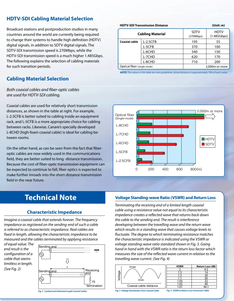
Coaxial cables are used for relatively short transmission distances, as shown in the table at right. For example, L-2.5CFB is better suited to cabling inside an equipment rack, and L-5CFB is a more appropriate choice for cabling between racks. Likewise, Canare’s specially developed L-8CHD (high-foam coaxial cable) is ideal for cabling be-tween rooms.
On the other hand, as can be seen from the fact that fiber-optic cables are now widely used in the communications field, they are better suited to long -distance transmission. Because the cost of fiber-optic transmission equipment can be expected to continue to fall, fiber optics is expected to make further inroads into the short-distance transmission field in the near future.
HDTV-SDI Transmission Distance (Unit: m)
Cabling Material (270Mbps)SDTV (1.485Gbps)HDTV L-2.5CFB 195 55 L-5CFB 370 100 L-6CHD 540 150 L-7CHD 620 170 L-8CHD 710 200 Coaxial cable
Optical fiber (single mode) 2,000m or more
NOTE: The values in this table are mere guidelines. Actual distance is approximately 70% of each value.
Technical Note
Vmax
Vmin
Voltage
Coaxial cable distance
Fig. 3 Voltage Distribution Over Coaxial Cable
VSWR Return Loss (dB) 2 9.5 1.5 14 1.2 20 1.1 26 1.05 32 1.02 40 1.01 46.1 R 75 Sending end
Sending end Receivingend
termination
Fig. 2 Limited and Unlimited Length Coaxial Cables Fig. 4 VSWR to Return Loss Conversion Table
Characteristic Impedance
Imagine a coaxial cable that extends forever. The frequency impedance as registered on the sending-end of such a cable is referred to as characteristic impedance. Real cables are fixed in length, allowing the characteristic impedance to be measured and the cables terminated by applying resistance of equal value. The
end result is the configuration of a cable that seems limitless in length. (See Fig. 2)
Voltage Standing-wave Ratio (VSWR) and Return Loss
Terminating the receiving end of a limited length coaxial cable using a resistance value not equal to its characteristic impedance creates a reflected wave that returns back down the cable to the sending end. The result is interference developing between the travelling wave and the return wave which results in a standing wave that causes voltage levels to fluctuate. The degree to which terminating resistance matches the characteristic impedance is indicated using the VSWR or voltage standing-wave ratio standard shown in Fig. 3. Going hand in hand with the VSWR ratio is the return loss factor which measures the size of the reflected wave current in relation to the travelling wave current. (See Fig. 4)
HD
-SDI D
istr
ibution
canar
e.c
om
Canare 75Ω coaxial cables
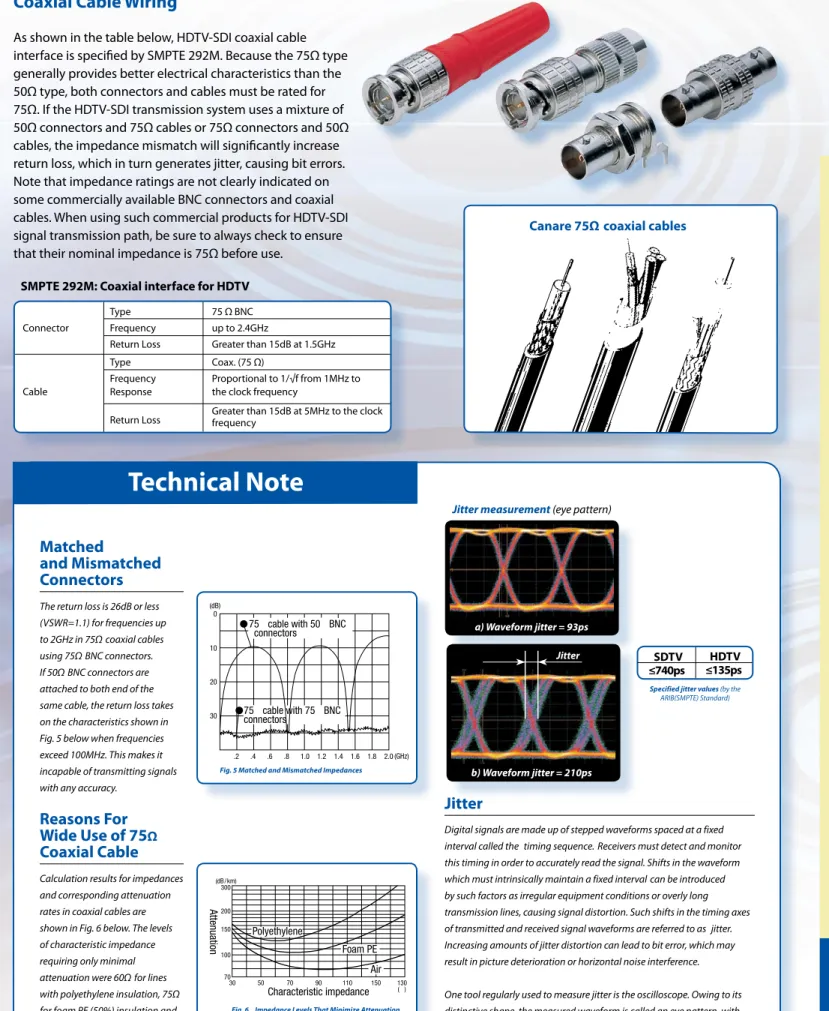
Coaxial Cable Wiring
As shown in the table below, HDTV-SDI coaxial cable interface is specified by SMPTE 292M. Because the 75Ω type generally provides better electrical characteristics than the 50Ω type, both connectors and cables must be rated for 75Ω. If the HDTV-SDI transmission system uses a mixture of 50Ω connectors and 75Ω cables or 75Ω connectors and 50Ω cables, the impedance mismatch will significantly increase return loss, which in turn generates jitter, causing bit errors. Note that impedance ratings are not clearly indicated on some commercially available BNC connectors and coaxial cables. When using such commercial products for HDTV-SDI signal transmission path, be sure to always check to ensure that their nominal impedance is 75Ω before use.
SMPTE 292M: Coaxial interface for HDTV
Type 75 Ω BNC
Connector Frequency up to 2.4GHz
Return Loss Greater than 15dB at 1.5GHz
Type Coax. (75 Ω)
Frequency Proportional to 1/√f from 1MHz to
Cable Response the clock frequency
Return Loss Greater than 15dB at 5MHz to the clock frequency
Specified jitter values (by the ARIB(SMPTE) Standard)
SDTV
≤740ps ≤135psHDTV
Fig. 5 Matched and Mismatched Impedances
30 20 10 0 (dB) .2 .4 .6 .8 1.0 1.2 1.4 1.6 1.8 2.0 (GHz) 75 cable with 75 BNC connectors 75 cable with 50 BNC connectors
Jitter measurement(eye pattern)
a) Waveform jitter = 93ps
b) Waveform jitter = 210ps Jitter
Jitter
Digital signals are made up of stepped waveforms spaced at a fixed interval called the timing sequence. Receivers must detect and monitor this timing in order to accurately read the signal. Shifts in the waveform which must intrinsically maintain a fixed interval can be introduced by such factors as irregular equipment conditions or overly long transmission lines, causing signal distortion. Such shifts in the timing axes of transmitted and received signal waveforms are referred to as jitter. Increasing amounts of jitter distortion can lead to bit error, which may result in picture deterioration or horizontal noise interference. One tool regularly used to measure jitter is the oscilloscope. Owing to its distinctive shape, the measured waveform is called an eye pattern, with the jitter expressed by the width of the area where the rising and falling edges of the waveforms cross each other. This jitter value is specified by the ARIB (SMPTE)Standard shown in the accompanying table.
Technical Note
Matched
and Mismatched
Connectors
The return loss is 26dB or less (VSWR=1.1) for frequencies up to 2GHz in 75Ω coaxial cables using 75Ω BNC connectors. If 50Ω BNC connectors are attached to both end of the same cable, the return loss takes on the characteristics shown in Fig. 5 below when frequencies exceed 100MHz. This makes it incapable of transmitting signals with any accuracy.
Reasons For
Wide Use of 75
ΩCoaxial Cable
Calculation results for impedances and corresponding attenuation rates in coaxial cables are shown in Fig. 6 below. The levels of characteristic impedance requiring only minimal attenuation were 60Ω for lines with polyethylene insulation, 75Ω for foam PE (50%) insulation and 95Ω for air insulation. This is why the 75Ω cable is used for longer distance transmissions.
Fig. 6 Impedance Levels That Minimize Attenuation Conditions outer conductor: copper braid; insulation O.D. 5mm inner conductor: solid copper: frequency 200MHz 70 30 50 70 90 110 150 130 100 150 200 300 ( ) Characteristic impedance Attenuation (dB/km) Polyethylene Foam PE Air
HD
-SDI D
istr
ibution
canar
e.c
om
HD-SDI Distribution :
Fiber-Optic Wiring
Fiber-Optic Wiring
As shown in the table below, High-definition serial digital interface is specified by SMPTE 292M. Although the fiber-optic cable may have excellent characteristics in terms of signal transmission, it may be liable to the influence of tension or bends that exceed its permissible range, as well as to humidity or dust. In particular, care must be exercised during installation, since tension is more apt to be applied to the interface. To ensure stable light signal transmission, be sure to handle the interface properly, and correctly clean the fiber-optic connectors.
FCF FCFR FCM FCF FCMR FCM HDTV Camera Hybrid fiber-optic receptacle cable FCS015A-FR Camera terminal panel Splice enclosure Outside Broadcast Van Rack Hybrid fiber-optic camera cable FCC**A
Outside Broadcast Van Hybrid fiber-optic camera cable
FCC**A Hybrid fiber-opticreceptacle cable FCS015A-MR
Fiber-optic cable reel
Base station
CCU
Fiber-Optic System Installation Example
SMPTE 292M: Optic fiber interface for HDTVFiber type Single mode
Connector Type SC/PC
Optical wavelength 1310nm≤40nm
Maximum spectrial line width between 10nm
half-power points Jitter 0.2UI Output power -12 to -7.5dBm Input power -7.5 to -20dBm Canare fiber-optic cable with SC connector Canare fiber-optic cord
Technical Note
Ferrule Alignment sleeves Cleaning stick Cleaning stickCLETOP 2.5/2.0Maintaining Fiber-Optic Hybrid Connectors
The connector sections to be cleaned are the key parts, including the tips and sides of ferrules, the interior walls of alignment sleeves and the interior and exterior of connector shells. Note that scratches and particles of foreign matter on the tip of the ferrule can have a disabling effect on fiber-optic transmission. The following procedures should be used when cleaning fiber-optic connectors.
• For Plugs, the interior surfaces of alignment sleeves and the tips of
ferrules are to be cleaned with the non-alcohol treated cleaning stick using a gentle stroking action. Canare FCF and FCFR enhance easy cleaning procedure for its innovative alignment sleeve and indulator detachable design.
• For Jacks, it is important to clean both the tips and sides of
the completely protruding ferrules with the cleaning stick.
• Both the male and female connector shells tend to attract dust
and metal particles, so it is important to clean both the insides and outsides using cotton gauze or similar material.
• Contact Canare for information on the recommended cleaning stick.
• The alignment sleeve (split sleeve) keeps the ferrules in highly
precise alignment with each other. After Cleaning
Before Cleaning
SMPTE 304M & 311M: Hybrid Electrical and Fiber-Optic Camera Connector & Cable
Optical Fibers Two units: Blue and Yellow, Single mode, 1310nm Auxiliary Conductors Two units: Black and White,
Cable DC loop resistance ≤43 Ω/km
Signal Conductors Two units: Red and Gray, DC loop resistance ≤184 Ω/km Overall Braid Shield DC resistance ≤20 Ω/km
Wavelength: 1100 to 1350nm
Optical Insertion loss: 0.5dB max.
Connector Return loss: Better than -45dB
Auxiliary electrical contacts AC 600V, 10A Low-voltage contacts AC 42V or DC 60V, 1A
HD
-SDI D
istr
ibution
canar
e.c
om
Fiber-optic φ3mm Coax L-5CFB φ7.7mmTechnical Note
EO/OE System Design
In EO/OE system design, 1) cable attenuation loss, 2) connector insertion loss, 3) fusion splice connection loss, and 4) Mux/DeMux insertion loss have to be calculated so that they are less than the loss budget (LB) of the optic link. For HD/SD-SDI system, since the Mux/DeMux loss is greater than that of the fiber attenuation loss, it would be essential you to consider such loss elements when you configure the system. Loss Budget (LB)
Loss Budget (LB)
Loss budget is the difference between the optical power output (P1) from the EO converter and the light reception sensitivity (P2) of the OE converter. LB = P1-P2 λ1 λ2 λ8 λ1 λ2 λ8 Fiber-Optic M u x D e M u x λ1+λ2+・・・+λ8 1471nm 1310nm 1611nm WDM WDM EO EO EO EO OE OE OE OE Optic Output Distance Optic Receiving Margin
Loss Budget Diagram
Loss Attenuation
Loss Factor Value
Connector Insertion Loss 0.5dB/Point Mux/De Mux 2˜3dB/Point WDM coupler 0.5dB/Point Fiber Cable 0.3dB/km(*) Splitter 0.5dB/Main 10dB/Branch Divider 3dB/Point Fusion Splice Loss 0.2dB/Point System Margin 3˜6dB
* 0.5˜1.0dB/km for Dark fiber u v w x Example If the optical power output P1 = -3dBm and the reception sensitivity P2 = -20dBm: LB = -3dBm - (-20dBm) = 17dB
Canare EO/OE Series on Distributing Hi-Def signals
High definition (HD) digital signals are becoming mainstream in broadcast stations and postproduction studios, and such facilities are rapidly being required to employ systems capable of handling HD digital signals. While conventional fiber-optic transmission equipment have been expensive, the cost of peripheral equipment has greatly decreased in recent years thanks to the widespread use of optical fiber transmission, resulting in broadcasting equipment shifting quickly to fiber-optic systems. People generally consider fi-ber-optic transmission to be too difficult to employ, however it can minimize transmission loss and enable systems to be designed with no special measures required to eliminate noise, which must always be kept in mind when installing coaxial cables. Canare Electric-to-Optic/Optic-to-Electric (Canare EO/OE) series will bring you to next level of potential, flexibility, and expandability at an affordable cost.
Advantage 1:
Flexible Layout
The maximum transmission distance for L-5CFB coaxial cable is ap-proximately 100 meters. Within this distance, however, ideal wiring routes may not be selected nor equipment installed in convenient locations during cable installation in rooms or between rooms. Since fiber-optic cable can transmit signal over distances of tens of kilo-meters, layouts can be more freely planned and centered on equip-ment without worrying about the wiring distance. This advantage cannot be overlooked.
Advantage 2:
Space Saving
Fiber-optic cables are generally 3mm of outer diameter, which is ap-proximately 2/5 that of L-5CFB coaxial cable and apap-proximately 1/6 the size in terms of cross-sectional ratio. Even when spaces under floors, in cable ladders, or component racks are full of coaxial cable and no more lines can be added, fiber-optic cables can cope with the situation.
Advantage 3:
Eliminating Electromagnetic Noise
As you know, unlike copper cable, fiber-optic cable is not susceptible to electromagnetic noise. Fiber-optic wiring will give you many op-tions - No more worrying about isolating to power lines and so on.
Advantage 4:
Easy to Add Lines without Re-Wiring
Coarse Wave Division Multiplexing (CWDM) technology enables multiple signals to be transmitted over “one” fiber-optic cable. Once the fiber-optic cable has been installed, additional cables are not necessary in your system upgrade. Canare CWDM can be transmit-ted up to 8 channels in “one” fiber. You will see Canare CWDM saving the total installation cost incredibly.
Coax
Fiber-optic Affected
Unaffected Noise