THE EMERGENCE OF THREE WORLDS OF WELFARE
Benjamin T. Danforth
A thesis submitted to the faculty of the University of North Carolina at Chapel Hill in partial fulfillment of the requirements for the degree of Master of Arts in the Department of Political Science.
Chapel Hill 2009
ABSTRACT
BENJAMIN T. DANFORTH: The Emergence of Three Worlds of Welfare (Under the direction of John D. Stephens.)
ACKNOWLEDGMENTS
TABLE OF CONTENTS
LIST OF TABLES . . . v
LIST OF FIGURES . . . vi
Introduction . . . 1
Conceptualizing the Welfare State . . . 3
Incorporating Public Provision of Social Services, Gender, and Activation 5 A Complete, Multidimensional Framework . . . 8
The Emergence of Three Worlds . . . 9
Data . . . 11
Methods . . . 15
Model-Based Cluster Analysis . . . 16
Agglomerative Hierarchical Cluster Analysis . . . 20
Results . . . 21
Discussion and Conclusions . . . 23
APPENDIX . . . vii
LIST OF TABLES
Table
1 Rank-Order of Welfare States in Terms of Combined Decommodification,
1980 . . . vii
2 Clustering of Welfare States According to Liberal, Conservative, and So-cialist Regime Attributes, 1980 . . . viii
3 Core Dimensions of the Three Welfare State Regimes . . . viii
4 Welfare State Clusters for 1952 and 1980 . . . ix
5 Measure Descriptions and Sources . . . x
5 Measure Descriptions and Sources . . . xi
5 Measure Descriptions and Sources . . . xii
6 Sets of Measures . . . xii
7 Possible Parameterizations of the Covariance matrix Σk and Their Geo-metric Features . . . xiii
8 Number of Distinct Clusters Detected For Each Set of Measures . . . xiii
9 Country Classifications for Measure Set A for Each Five-Year Interval from 1950–1995 . . . xiv
10 Country Classifications for Measure Set B for Each Five-Year Interval from 1960–1995 . . . xv
11 Country Classifications for Measure Set C for Each Five-Year Interval from 1970–1995 . . . xvi
12 Country Classifications for Measure Set D for Each Five-Year Interval from 1980–1995 . . . xvii
13 Country Clusters for Measure Set A for Each Five-Year Interval from 1950–1995 . . . xviii
14 Country Clusters for Measure Set B for Each Five-Year Interval from 1960–1995 . . . xix
15 Country Clusters for Measure Set C for Each Five-Year Interval from 1970–1995 . . . xx
LIST OF FIGURES
Figure
1 Dendrograms with P-Values for Measure Set A – 1950 and 1955 . . . xxii
2 Dendrograms with P-Values for Measure Set A – 1960 and 1965 . . . xxiii
3 Dendrograms with P-Values for Measure Set A – 1970 and 1975 . . . xxiv
4 Dendrograms with P-Values for Measure Set A – 1980 and 1985 . . . xxv
5 Dendrograms with P-Values for Measure Set A – 1990 and 1995 . . . xxvi
6 Dendrograms with P-Values for Measure Set B – 1960 and 1965 . . . xxvii
7 Dendrograms with P-Values for Measure Set B – 1970 and 1975 . . . xxviii
8 Dendrograms with P-Values for Measure Set B – 1980 and 1985 . . . xxix
9 Dendrograms with P-Values for Measure Set B – 1990 and 1995 . . . xxx
10 Dendrograms with P-Values for Measure Set C – 1970 and 1975 . . . xxxi
11 Dendrograms with P-Values for Measure Set C – 1980 and 1985 . . . xxxii
12 Dendrograms with P-Values for Measure Set C – 1990 and 1995 . . . xxxiii
13 Dendrograms with P-Values for Measure Set D – 1980 and 1985 . . . xxxiv
Introduction
Beginning with Gøsta Esping-Andersen’s seminal typology of welfare capitalism, sig-nificant scholarly attention has been devoted to classifying contemporary welfare states (Esping-Andersen 1990). Although he was not the first to develop a framework for comparing welfare states (e.g., see Titmuss 1958), Esping-Andersen was the first to systematically show that welfare states can be grouped by distinct, real-world mod-els. Specifically, in his typology, Esping-Andersen identifies three types of welfare state regimes by which advanced capitalist democracies can be categorized: liberal, conserva-tive, and social democratic.
This tripartite typology has served as the conventional lens for welfare state com-parison, but it has also been the target of a number of major refinements. Three such refinements include the addition of dimensions for the public provision of social services, gender egalitarian, or defamilializing, policies, and the mobilization, or activation, of labor. Even with the incorporation of these three refinements, Esping-Andersen’s ty-pology has been shown to be fairly robust in distinguishing between the three welfare state regimes (Edwards 2003). A fourth refinement, which comes from the literature on varieties of capitalism, further augments the tripartite typology by positing two types of production regimes: liberal market economy and coordinated market economy, with “continental” and “Nordic variants” of the latter type (Hall and Soskice 2001; Pontus-son 2005). Despite initially being presented as somewhat of an alternative to Esping-Andersen’s state-centered system of classification, the production regime typology has actually been shown to be highly complementary to the welfare state typology (Ebbing-haus and Manow 2001; Huber and Stephens 2001; Iversen and Stephens 2008). In fact, the combination of the two typologies into a single framework provides a more accurate conceptualization of Esping-Andersen’s worlds of welfare capitalism.
wel-fare capitalism using cross-sectional data from 1980, but did these distinct worlds exist prior to this time point? In other words, when exactly did advanced capitalist democra-cies crystallize into three distinct worlds of welfare capitalism? Power resources theory, which has become the dominant approach to the study of welfare state development, has focused on the causes rather than the timing of consolidation. A partial yet promi-nent exception is Alexander Hicks’ comparative historical analysis of key social-security programs in 15–18 advanced industrialized countries from 1880 to 1990 (Hicks 1999). In his analysis, Hicks finds that many of the countries classified by Esping-Andersen as social democratic welfare states in 1980 had consolidated social-security programs by 1952 while many of those classified as conservative and liberal did not. Interestingly, Hicks notes that the three earliest consolidators were all liberal welfare states in 1980: Australia, New Zealand, and the United Kingdom. Beyond 1952, however, Hicks’ analy-sis provides little insight on the coalescence of advanced welfare states into three discrete groups of welfare capitalism.
In this paper, I seek to establish the point in history when three distinct welfare state regimes first emerged, thus bridging Hicks’ and Esping-Andersen’s analyses. To determine this point in history, I use two methods of cluster analysis—model-based clus-ter analysis and agglomerative hierarchical clusclus-ter analysis—to systematically analyze welfare state features for 18 OECD countries from 1950 to 1995. The core dimensions that I will focus on include: decommodification; the public provision of social services; stratification, which is reconceptualized as population coverage, income redistribution, and post-tax/transfer poverty; defamilialization; and activation. Due to theoretical con-siderations and data limitations, these core dimensions are not analyzed equally for the 45-year period under consideration. For similar reasons, I will not include a dimension for production regimes in my analysis at all. Given this purposeful omission, my analysis will not directly account for the emergence of three worlds of welfare capitalism per se but rather three worlds ofwelfare state regimes.1
Besides ascertaining the point in history when three welfare states regimes first emerged, this paper also aims to connect the historical development of welfare state
1
clusters with prominent explanations of welfare state consolidation. One such explana-tion emphasizes the role of political accumulaexplana-tion in spurring the emergence of distinct welfare state regimes. Drawing on power resources theory, political accumulation has been conceptualized as the long-term partisan composition of government (Huber, Ra-gin, and Stephens 1993; Huber and Stephens 2001). Given that there has been significant variation in long-term partisan trends across the countries being analyzed, this expla-nation implies that welfare states should become more distinctive over time. Another notable explanation, which partly interacts with the first, holds that “increasing return,” or self-reinforcing, processes of welfare state development should lead to the emergence of multiple distinct welfare state equilibria (Pierson 2000). This explanation, which is often referred to as path dependence, not only entails that discrete groupings of welfare states should emerge but also that these groupings should become relatively stable over time, both in terms of number and membership. As will be discussed in grater detail, the empirical evidence presented in this paper provides support for both of these historical institutional explanations.
Conceptualizing the Welfare State
Esping-Andersen’s Three Worlds
The welfare state has long been a topic of interest in comparative politics and po-litical sociology, but it was not until Esping-Andersen’s breakthrough work on the topic that scholars seriously began to consider and evaluate multiple dimensions and multiple types of welfare states (Esping-Andersen 1990). In his work, Esping-Anderson breaks from the prior literature on the subject by recognizing that the welfare state is not just a minimal set of social-ameliorating policies and that social expenditure levels offer a poor basis for welfare state comparison. With these shortcomings in mind, Esping-Andersen reconceptualizes the welfare state as having two key dimensions: decommodification and stratification. Decommodification represents the degree to which the social rights granted by the welfare state enable an individual (or family) to maintain a livelihood without relying on the market.2 Stratification, on the other hand, refers to the social
2
ordering that is embedded in and reinforced by the welfare state. To measure these dimensions, Esping-Anderson develops a number of indices that not only tap the expen-diture levels of social provisions but also the eligibility requirements, coverage, targeting, and public-private mixtures associated with these provisions. Finally, drawing on this last point, Esping-Andersen stresses the need to look at the interaction between the welfare state and the other two main sources of social provisions, namely the family and the market, to fully ascertain the decommodifying and stratifying features of the welfare state.
When Esping-Andersen uses the two welfare state dimensions, decommodification and stratification, in a cross-country analysis of advanced capitalist democracies, he demonstrates that there is not one universal welfare state model. Instead, Esping-Andersen identifies three salient types of what he terms as welfare state regimes. Each of these welfare state regimes represents a discrete logic of welfare state organization, stratification, and integration in a broad societal context. Esping-Andersen labels the three regime types as liberal, conservative, and social democratic, which reflect their distinct historical origins and developmental trajectories.
The liberal welfare state regime relies heavily on the market for the provision of social benefits and services, with the state providing support only to those who cannot support themselves in the market. This regime is built on liberal work-ethic norms and thus its state-provided benefits tend to be modest and restricted, with a strong emphasis on means-testing and strict eligibility requirements. In order to further limit state welfare obligations, there is an active encouragement of private welfare schemes. Given the residual nature of this regime, it is only weakly decommodifying. It also leads to a dualistic social order, with a minority dependent on state welfare and a majority reliant on market-differentiated welfare.
benefits are delivered through social insurance schemes that are organized according to narrow, occupation-based solidarities. The regime’s emphasis on upholding class differences limits its decommodifying impact.
The social democratic welfare state regime seeks to emancipate the individual from both the family and the market through generous and universal state-sponsored social rights. Firmly rooted in social democracy, this regime gives high priority to social equality and economic redistribution and strives to secure its citizens’ welfare for the entire life course, from the cradle to the grave. To foster universal solidarity in favor of the welfare state, some social benefits are graduated according to earnings. Although this regime is highly decommodifying, it is also highly committed to full employment, mainly out of necessity to financially sustain itself.
These three regime types form the cores of the worlds of welfare capitalism envisioned by Esping-Andersen. In his empirical analysis, Esping-Andersen shows that these regime types do seem to correspond with real-world clusters of countries in 1980 (see Tables 1 and 2). As the remaining discussion points out, however, Esping-Andersen’s concep-tualization and analysis do suffer from a number of key deficiencies that warrant being addressed.
Incorporating Public Provision of Social Services, Gender, and Activation
Although Esping-Andersen’s tripartite typology of welfare state regimes is widely considered an insightful breakthrough, it has not been immune to criticism. To the contrary, Esping-Andersen’s typology has been at the center of a lively and productive body of scholarship that aims to expand and improve welfare state categorization and comparison. One thread in this literature has focused on identifying additional regime types, particularly for welfare states in Southern Europe and Eastern Europe (Leibfried 1993; Ferrera 1996; Gans-Morse and Orenstein 2008).4 Nearly all of the new regime types established by this body of work are, however, products of the third wave of democratization of the 1980s and 1990s and thus postdate Esping-Andersen’s three
4
regime types for 1980. For this reason, these new regime types are not discussed further or incorporated into this study. A second thread has sought to revise and supplement Esping-Andersen’s welfare state dimensions, with a particular emphasis on the public provision of social services, gender, and activation. According to this body of work, these three dimensions are not secondary elements but core features of the welfare state. In order to better differentiate the social democratic regime from the other two regime types, a number of scholars have pushed for the inclusion of public social services into the multidimensional framework of welfare state regimes. Although Esping-Andersen expressly aims to take a holistic approach to welfare state comparison, much of his anal-ysis of welfare state differences is centered around old-age, sickness, and unemployment cash benefits (i.e. transfer payments). It has been pointed out, however, that a key distinguishing feature of the social democratic regime type is its emphasis on the public financing and delivery of social services (Huber and Stephens 2001). As Scharpf and Schmidt (2000) argue, this feature represents a critical piece of information for accurately dividing the country groupings for the social democratic and conservative regime types. This is the case because these two regime types largely differ in how they organize their “caring” services: the social democratic regime type, as stated before, prefers profession-alized public solutions while the conservative regime type favors informal, family-based solutions (Scharpf and Schmidt 2000). In effect, the absence of a dimension for the pub-lic provision of social services in Esping-Andersen’s original typology makes it incapable of fully secerning social democratic welfare states from conservative ones.
allowances, parental leave schemes, child and elderly care provisions, active labor mar-ket policies, and other gender egalitarian policies guaranteed by a welfare state are all crucial determinants of women’s economic independence. In light of these substantial linkages, gender has become increasingly incorporated into welfare state classifications and analyses.
In response to the critiques regarding gender, Esping-Andersen has tweaked his con-ceptualization of the welfare state to include a new dimension that better captures gen-der relations (Esping-Angen-dersen 1999). Following the lead of several feminist scholars, Esping-Andersen tags this dimension as “defamilialization,” which is meant to draw at-tention to the welfare state’s role in reshaping family patterns and bestowing social rights to individuals (Sainsbury 1996). From a gender perspective, defamilialization gauges the degree to which social policies enable women to sustain households independent of the family. When this new dimension is used to look at cross-country gendered outcomes, patterns emerge that correspond with Esping-Andersen’s original tripartite typology (Sainsbury 1999; Gornick and Meyers 2003; Huber et al. 2005). In other words, the addition of a gender-oriented dimension to Esping-Andersen’s conceptual framework of the welfare state does not diminish but strengthens the explanatory power of his regime types.
two, particularly the conservative regime. Although decommodification alone is suffi-cient to differentiate between the social democratic and liberal regimes, activation as well as public social services and gender are needed to clearly distinguish between the social democratic and conservative regimes.
A Complete, Multidimensional Framework
Building on Esping-Andersen’s original typology and the prominent conceptual re-finements made to it, a more complete and comprehensive typological framework of the three worlds of welfare can be constructed. In this section, I present such a framework (see Table 3). The dimensions used to derive this framwork are later used to inform my selection of measures for analysis. To some degree, these dimensions will also be employed as benchmarks to determine the timing and sequencing of welfare state crys-tallization after 1950.
state involvement is, to a large extent, captured by post-tax/transfer poverty. I contend that these three separate dimensions better capture the impact that each welfare state regime has on social stratification and inequality than a single, amalgamated dimension. As mentioned before, I have purposefully omitted production regime as a dimension in this typological framework. Welfare state regimes and production regimes have been shown to be mutually enabling in a number of ways, and they do share some common historical origins, particularly with respect to the strength of union organization. But, to a good extent, these two groups of regimes have evolved in different ways, at different speeds, and for different reasons. For instance, cross-national differences in contempo-rary industrial-relations systems, which are core parts of the production regimes, reflect cross-national differences in the strength and scope of employer organizations during the early 20th century (Crouch 1993). In a similar vein, cross-national differences in contemporary training regimes can be traced back to 19th-century traditions of coop-eration and coordination (Thelen 2004). As these examples highlight, contemporary production regimes are largely products of long historical relationships between working class movements and employers. This contrast with the more recent story of welfare state development, which is largely driven by a struggle over taxation between social demo-cratic forces and their conservative counterparts (Swenson 1991; Iversen and Stephens 2008).
From a practical standpoint, the inclusion of production regime as a dimension is also problematic because it is in itself a complex, multidimensional concept and it does not readily lend itself to quantitative operationalization. So, while acknowledging that production regimes are integral components of the three worlds of welfare capitalism, I do not aspire to trace their historical development into distinct types. Rather, I will focus my analysis on the historical emergence of three types of welfare state regimes, which are defined by the seven dimensions listed in Table 3.
The Emergence of Three Worlds
concrete knowledge as to when the welfare states of advanced capitalist democracies first crystallized into separate liberal, conservative, and social democratic clusters. In-stead, most historical analysis of the three welfare state regime types has dealt with the question of their origins: why have separate regime types emerged? From this analysis, several theoretical approaches have emerged, with power resources theory being the most prominent and widely used approach.5 According to this approach, the distribution of organizational power between labor organizations and left parties on one side and right-wing political forces on the other side serves as the primary determinant of differences in welfare state development across countries and over time (Stephens 1979; Huber and Stephens 2001). This is the approach that Esping-Andersen adopts in his explanation of why there are different, real-world models of welfare capitalism. But with so much focus on answering the question of why, the question of when has fallen to the wayside. The main contribution of this research project will be to address this latter question by systematically examining the histories of welfare states to determine when they first constellated into three distinct welfare state regimes.
of these two studies is not to identity clusters of welfare states but rather “families of nations,” which are conceptually more encompassing than welfare state regimes.
Although no prior studies have been able to pinpoint the time at which welfare states coalesced into three distinct groupings, the empirical work done by Esping-Andersen (1990) and Hicks (1999) provides some broad clues (see Table 4). In first identifying the existence of three worlds of welfare state regimes, Esping-Andersen uses cross-sectional data from 1980, which implies that the three welfare state regime types had crystallized by this point. As discussed earlier, however, Esping-Andersen’s seminal analysis uses a more narrowly defined framework for his clustering, which thus casts some doubt on his identification of three delineated clusters for 1980.6 At the same time, Esping-Andersen does not thoroughly discuss or investigate whether the three worlds emerged prior to 1980, except to say that the three worlds did not exist prior to 1950 (1999, 53).7 Moving further back in history, Hicks identifies two clusters of welfare states for 1952 based on whether each welfare state had implemented five major types of income maintenance programs: pensions; sickness, disability, and unemployment insurances; and family allowances. Again, despite using a very narrow conceptualization of welfare state regimes, Hicks’ clusters of consolidators and non-consolidators indicate that the three worlds did not emerge until after the 1950s. Together, these two sets of findings suggest that the three welfare state regimes crystallized after 1950 and perhaps by 1980.
Data
In order to locate historically when the three worlds of welfare first emerged, I an-alyze the welfare states of 18 advanced capitalist countries using the multidimensional framework described in Table 3 for each five-year interval from 1950 to 1995 inclusive.8
The measures for this framework are primarily drawn from the Social Citizenship Indi-cator Program (SCIP), which is the main data set utilized by Esping-Andersen inThree
6A common critique of Esping-Andersen’s work is that his own analysis does not produce clear-cut clusters. For example, looking at the Esping-Andersen’s reproduced results in Table 1, the cut points between the three clusters of welfare states appear somewhat arbitrary.
7
It is not even clear why Esping-Andersen chooses to look at 1980 because he offers little discussion on his selection of data.
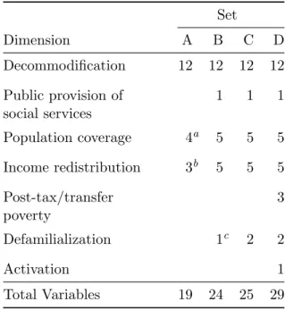
Worlds of Welfare Capitalism.9 29 measures are used to tap the seven welfare state dimensions, though data for all of these measures are not available for the entire 45-year range of history under study. Beginning in 1950, data are limited to 19 measures for three dimensions, but with each subsequent decade, additional measures become avail-able and are thus utilized. By 1980, data are availavail-able for all of the chosen measures for all seven dimensions.10 In essence, four different sets of measures—each more extensive than the one preceding it—are derived from the data for the purpose of analysis. These four sets are labeled A, B, C, and D. See Table 5 for an overview of the measures and their sources and Table 6 for a breakdown of which measures comprise each set.
The decommodification dimension is operationalized as 12 measures, all of which come from the SCIP data set and are available for the entire period from 1950–1995. Three of these measures are the standard net replacement rates for an individual average production worker (APW) for three basic social-insurance programs: old-age pensions, sick pay, and unemployment insurance. The minimum old-age pension, represented as the net replacement rate for an individual APW, is also included. Together, these re-placement rates summarize the degree to which the cash benefits approximate a worker’s expected market-based income. In order to capture benefit conditionality, the number of years (or weeks) of contributions to qualify for the entitlements are used in addition to the share of the benefit financed by worker contributions for old-age pensions and the number of waiting days to receive sick pay and unemployment insurance. Lastly, the number of weeks of benefit duration for sickness and unemployment are included to represent the maximum duration of these entitlements. All of these measures are equiv-alent to those used by Esping-Andersen to construct his unweighted decommodification indices in The Three Worlds of Welfare Capitalism(1990).11
9
The Social Citizenship Indicator Program was formerly known as theSvensk Socialpolitik i Interna-tional Belysning(SSIB). The other five data sets used in this paper include: the Comparative Welfare States Data Set; the Standardized World Income Inequality Database (SWIID), the Luxembourg In-come Study (LIS); the Comparative Maternity, Paternal, and Childcare Database; and the OECD’s Social Expenditure Database (SOCX).
10The historical discrepancy in data availability for the seven dimensions is largely due to the limited scope of past data-collection efforts, but it may also be indicative of trends in welfare state development. In other words, data may have not been collected on defamilialization and activation in the initial decades of the post-war era because these dimensions of the welfare state had not yet developed or been articulated.
One measure, the total civilian government employment as a percentage of the working-age population, is used to quantify the public provision of social services. This measure serves as a proxy for the amount of state involvement in the delivery of social services, like health care, education, and personal care. Of course, this measure also includes civilian government employees in non-welfare sectors, but it has been pointed out that nearly all variations in civilian public employment across countries and time can be accounted for by welfare state employment (Huber and Stephens, 2001a: 51). This measure is available from 1960 onward.
Two sets of indicators are used to measure population coverage, the first of which captures social-insurance coverage while the second summarizes social-service coverage. The first set of indicators is comprised of the coverage rates for the old-age pensions, sick pay, and unemployment insurance. These coverage rates are calculated as the percentage of the labor force, ages 16–64, that is entitled to receive the benefits upon fulfilling basic eligibility conditions. The take-up rate for pensions—the percentage of the pension-age population that receives pensions—is also incorporated into this set of indicators. These same measures are used by Esping-Andersen to weight his decommodifiication indices and compute a summary measure of “average universalism” (Esping-Andersen 1990, 54, 78). The second set of indicators has only one member: the public share of total expenditures on health care as a percentage of GDP. This measure provides a good approximation of population coverage because public spending on health care is generally a function of the universalism of publicly provided health care. The first set of measures is available for the entire period of history being analyzed while the last measure is only available from 1960 on.
As measures of income redistribution, I use Esping-Andersen’s summary measure of benefit equality for each social-insurance program as well as Gini indices for gross and net income inequality. The benefit equality measures are calculated as the ratio between the standard and maximum replacement rates for an individual APW for old-age pensions, sick pay, and unemployment insurance (Esping-Andersen 1990, 78).12 The
12
Gini indices for gross and net income inequality consist of data from the World Income Inequality Database (WIID) that have been systematically standardized using the higher quality but more limited data from the Luxembourg Income Study (LIS) (Solt 2009). In conjunction with benefit equality measures, these two indices summarize the ability of welfare states to reduce income inequality, particularly through transfer payments. Data for the first three measures are available from 1950 onward and the later two measures for 1960 and afterward.
The measures for post-tax/transfer poverty are three relative poverty rates computed from the LIS, with the poverty threshold set at 50% of the net (i.e. post-tax/transfer) equivalized median disposable income. The first relative poverty rate covers the total population while the second and third focus on two vulnerable sub-populations, namely children (those under 18 years old) and the elderly (those over 64 years old). Although these three rates do not capture the absolute extent to which poverty is reduced, they do reflect the capacity of welfare states to maintain low poverty rates. Due to the limited historical scope of the LIS data set, these measures are only available for 1980 and beyond.13
The final two dimensions, defamilialization and activation, are measured using three variables: female labor force participation, parental leave generosity, and active labor market policies (ALMP). Female labor force participation—the percentage of women aged 15–64 who are employed or seeking work—is partly a function of welfare poli-cies that help women achieve work–family balance. Although it does not directly or fully gauge the defamilializing efforts of welfare states, this measure is included for its relatively extensive temporal range, starting in 1960. A better measure of defamilializa-tion, parental leave generosity, is also used to assess defamilializadefamilializa-tion, though it is only available from 1970 onward. This measure is the average replacement rate for parental leave for a 52-week period. For cases in which the leave period is longer than 52-weeks (Sweden in 1990 and 1995), the data are adjusted to fit this annual scale. Finally, the last variable is the total spending on ALMP as a percentage of GDP, with this quotient (0.95 and above).
13
weighted by the proportion of the population that is unemployed. This measure rates the activation efforts of welfare states and is only available for 1980 and afterward.
Many of the measures described above have, in part, been chosen for their historical completeness, but there are still a few instances of missing data. The proportion of miss-ingness ranges from 0.29% to 5.94% of the total data across the 10 cross-sections under analysis. In order to preserve the existing data and permit effective cluster analysis, the missing data points are estimated using nearest neighbor averaging (Troyanskaya et al. 2001).14 This method is superior to other single imputation approaches because it does not assume that all observations are members of a single group or drawn from one probability distribution. In other words, it is well suited to handle missingness in data that are suspected to be clustered. Like all single imputation methods, however, near-est neighbor averaging does not accurately reflect the uncertainty surrounding imputed values. Unfortunately, an imputation method for cluster analysis that is as robust as multiple imputation for linear models has not yet been fully developed.
Methods
In order to discern when three distinct types of welfare state regimes first crystal-lized, I implement two methods of cluster analysis: model-based cluster analysis and agglomerative hierarchical cluster analysis.15 Generally speaking, cluster analysis is a multivariate statistical technique that partitions data into subsets (i.e. clusters) of sim-ilar objects. Ideally, these clusters exhibit high internal homogeneity (members within clusters are very similar) as well as high external heterogeneity (members in each cluster are very dissimilar to those in other clusters). Model-based cluster analysis, which is rooted in probability theory, represents a more rigorous approach to identifying clusters, but it only performs well when clusters are relatively distinct. Agglomerative hierarchi-cal cluster analysis, which is based on distance, is capable of recognizing more tentative clusters, but it does not produce as reliable results. Used together, these two approaches can detect both strong and weak welfare state clusterings for each of the five-year
in-14
This process, which is implemented in theimputepackage for R, proceeds by finding thek nearest neighbors of an observation with missing values using the Euclidean metric. The missing values are then imputed by averaging the relevant elements of the nearest neighbors. For this paper,kis set at 4.
15
The cluster analyses in this paper have been conducted using themclustandpvclustpackages forR
tervals examined in this paper from 1950 through 1995. For the sake of comparability, analysis is done on each of the four sets of measures (A, B, C, D) for the all of intervals that they are available.
Model-Based Cluster Analysis
Mixture Model Estimation with Bayesian Regularization
The core assumption of model-based cluster analysis is that data are generated by a finite mixture of probability distributions, which each component representing a different group or cluster. Given a set of observations x = (x1, ..., xn), the density function can be expressed as
f(x) = n
Y
i=1
G
X
k=1
τkfk(xi|θk), (1)
wherefk(·|θk) is a probability distribution with parametersθk,τkis the probability that an observation belongs to the kth component, and G is the total number of compo-nents. As is conventionally done, I assume that each fk(·|θk) is a multivariate normal (Gaussian) density function, withθk consisting of two parameters: mean vector µk and covariance matrix Σk.16 Under this specification, the components of the mixture model are ellipsoidal in shape and centered at their means, µk.
Banfield and Raftery (1993) have extended this model-based framework for cluster-ing by reparametrizcluster-ing the covariance matrix in a form that permits variation in the orientation, shape, and volume of the components or clusters. This new form expresses the covariance matrix of thekth component as
Σk=λkDkAkDkT, (2)
whereDk is the orthogonal matrix of eigenvectors,Ak is a diagonal matrix proportional to the eigenvalues, and λk is a scalar. Using this formulation, the geometric features of the components can be allowed to vary. For each component k, Dk determines the
16
The density for the multivariate normal has the following form
φ(xi|µk,Σk)≡
expˆ −1
2(xi−µk)
T
Σ−k1(xi−µk)
˜
(2π)n2(Σk)12
orientation, Ak determines the shape, and λk determines the volume. By selectively re-stricting these parameters to be constant across all components, it is possible to derive a number of different covariance parameterizations with unique combinations of geometric features. Table 7, which is reproduced from Fraley and Raftery (2007b), lists possible covariance parameterizations and their geometric features.
A common approach to estimating the mixture models used in model-based clustering is to use the Expectation-Maximization (EM) algorithm, a two-step iterative estimation process (Dempster, Laird, and Rubin 1977). The first step, the E-step, uses estimates of the component means µk, covariance matrices Σj, and mixture proportions τj to compute the conditional probability that observationibelongs to the jth component.
zik=
τkφ(xi|µk,Σk)
PG
j=1τjφ(xi|µj,Σj)
, (3)
whereφ(·) is the multivariate normal distribution.17 Using this conditional probability, the M-step estimates a new set of parameters from the data. This two-step process is repeated as many times as needed until the difference in the parameter updates becomes arbitrarily small and convergence is thus reached. At this point, each observation is assigned to the component for which it has the highest posterior probability of being a member.
Despite its relative simplicity, it is not uncommon for the EM algorithm to fail to converge for mixture models, generally because of singularity in the covariance matrix. If singularity exists, the EM algorithm can be expected to diverge to a point of infinite likelihood.18 More specifically, the likelihood approaches infinity if the global optimum places a component on a single data point and sets the covariance for that component to 0.19 Issues of singularity are most likely to appear in models with a large number of components and models in which the covariance matrix is allowed to vary between components.
In order to avoid degeneracy in the estimation of mixture models, Fraley and Raftery 17In effect, the classification of observationiis treated as missing data.
18
This is based on the assumption that the likelihood is not bounded, as is generally the case for mixture models.
(2007a) propose using the maximum a posteriori (MAP) estimate from a Bayesian anal-ysis. By treating the Gaussian form of Equation 1 as a likelihood function and assigning a prior distribution to it, the problem of estimation failure due to singularity is elim-inated. Based on this approach, which is often referred to as Bayesian regularization, the posterior predictive density is assumed to be of form
π(τk, µk,Σk|x)∝L(x|τk, µk,Σk)p(τk, µk,Σk|θ), (4)
whereL(x|τk, µk,Σk) is the mixture likelihood function
L(x|τk, µk,Σk) = n
Y
i=1
G
X
k=1
τkφ(xi|µk,Σk), , (5)
and p(τk, µk,Σk|θ) is the prior distribution on the parameters τk, µk, and Σk, with θ representing other parameters. Adhering to recommendations made by Fraley and Raftery (2007a), I use a conjugate prior, with a normal prior on the mean that is conditional on variance
µ|Σ∼ N(µp,Σ/κp), (6)
and an inverse Wishart prior on the covariance matrix
Σ∼inverseWishart(νp,Λp), (7)
whereµp,κp,νp, and Λp are the mean, shrinkage, degrees of freedom, and scale, respec-tively.20 For the analyses in this paper, these four hyperparameters are assigned the following values: µp = the mean of the data; κp = 0.4;νp = the dimension of the data (d) + 2; and Λp = 10 or 20.21 These values make the prior very diffuse, thus ensuring 20See Fraley and Raftery (2005; 2007a) for the analytical solutions for the mean and variance at the MAP. They have derived solutions in the multivariate case for both inverse gamma and inverse Wishart conjugate priors.
21Two of these hyperparameters,µ
pandνp, have values that are recommended by Fraley and Raftery
(2007a; 2007b). The value forκp, which represents the addition of a fraction of an observation to each
component, was determined through experimentation. The values for Λpare significantly larger than
those recommended by Fraley and Raftery, leading to a more diffuse distribution. Λpis set to 10 for the
cross-sections before 1980 and to 20 for the cross-sections for and after 1980: the increase is needed to compensate for the addition of many measures in 1980.
Generally, Λp is a matrix, but when the covariance matrix is constrained to be spherical (the
that any inferences made from the posterior density will mostly be driven by the data. Once the posterior density described in Equation 4 is fully specified, the EM algo-rithm can used to estimate the posterior mode or MAP (maximum a posterior), which replaces the conventional maximum likelihood estimate.
Model Selection Using the Bayesian Information Criterion
Following a model-selection strategy developed by Fraley and Raftery (1998), mixture-model estimation can be used to detect the number of clusters and their features in set of data. First, a maximum number of clusters or components,Gmax, and a set covariance
parameterizations for Gaussian mixture models are chosen for consideration. Second, parameters are estimated using EM for each possible combination of the covariance pa-rameterizations and the number of components up toGmax.22 Third, a slightly modified
Bayesian Information Criterion (BIC) is computed for each model estimated in the prior step.23 Finally, the optimal number of components and covariance parameterization is determined by selecting the model for which the BIC is negatively maximized.
For the purposes of this study, the maximum number of components is limited to eight components and the set of covariance parameterizations is constrained to spherical and diagonal types. These values are chosen to reduce the chance of estimation failure due to singularity, which is a concern given that the number of dimensions in the data (ranging from 19 in 1950 to 29 in 1980 and beyond) exceeds the number of observations (18 countries). To further help ensure convergence and be consistent in terms of data preprocessing, all measures are standardized to have zero means and unit standard deviations.
22
Following Fraley and Raftery’s (2007a) suggestion, the conditional probabilities generated by model-based hierarchical clustering are used as the initial values for the EM process.
23Typically, the BIC has the form
BIC≡2loglikM(x, θ ∗
k)−(# params)Mlog(n),
where loglikM is the maximized log-likelihood for model Mand the given data, (# params)M is the
Agglomerative Hierarchical Cluster Analysis
As a complement to the model-based approach to clustering, I employ the more conventional technique of agglomerative hierarchical cluster analysis. In this approach to classification, data are not partitioned into a particular number of clusters in a single step, but rather they are assigned to clusters through a successive process. This method is termed “agglomerative” if the analysis starts with one-member or singleton clusters that are in turn merged into increasingly larger clusters. The end result of this process is a hierarchy of clusters, which is often presented graphically as a dendrogram.24
Of the many agglomerative procedures that are available, I use Ward’s method in my analyses. In this method, the fusion of two clusters is based on their combined error sum of squares (ESS), with the objective being to minimize this criterion in each successive step.25 As the measure of distance between clusters, I choose the Euclidean metric. Under these specifications, identified clusters tend to be spherical in shape and have equal volumes. Together, Ward’s method and the Euclidean metric represent the most frequently used agglomerative clustering technique.
In order to eliminate the effect of different measurement scales on clustering decisions, I standardize all measures before analysis. A well-known issue with hierarchical cluster analysis is the sensitivity of its results to different scales of measurement—measures with larger scales are more decisive in determining clusters than those with smaller scales. A common solution to this problem, which I adopt for my analyses, is to standardize all measures to unit variance.
Although interpreting the dendrograms produced by hierarchical clustering methods is often seen as a subjective process, it is possible to generate measures of uncertainty for these graphical results. Specifically, bootstrap resampling techniques can be used to estimate the probability that each cluster is supported by the data. A conventional bootstrapping approach can be used to compute the bootstrap probability (BP), which represents the frequency with which a cluster appears in the bootstrap replicates. This technique is considered inferior to a more advanced based multi-scale bootstrap
re-24
The “leaves” of this tree-like graphic are singleton clusters, the nodes constitute successive multi-member clusters, and the “branches” represent the distance between successive clusters.
25
sampling, which produces approximately unbiased (AU) probability values (Suzuki and Shimodaira 2006). Both of these p-values are calculated and reported for each edge of each dendrogram.
Results
Table 8 presents the optimal number of distinct clusters detected by model-based cluster analysis for each five-year interval from 1950–1995 for each set of measures. More detailed results, including country classifications and classification uncertainties, are reported in Tables 9–12 by measure set. To better show how the 18 countries are clustered in each iteration of the analysis, the countries classifications by measure set and interval are reproduced in Tables 13–16. Figures 1–14 contain the dendrograms generated by agglomerative hierarchical cluster analysis, again broken down by measure set and interval.
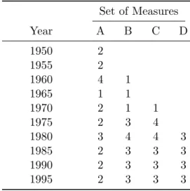
The summary results reported in Table 8 indicate that the three worlds of welfare were first emerging by 1975, became more pronounced by 1980, and were relatively stable by 1985. Two worlds are discernible in 1950 and 1955, but from 1960 up through 1970 there is no evidence to suggest the formation of a third world. In fact, during the 1960–1970 period, many of the results suggest the presence of only one cluster, which essentially indicates the absence of any meaningful, discrete country groupings. By 1985, however, the 18 countries have coalesced into three distinguishable worlds, an arrangement that remains static up through the last interval, 1995.
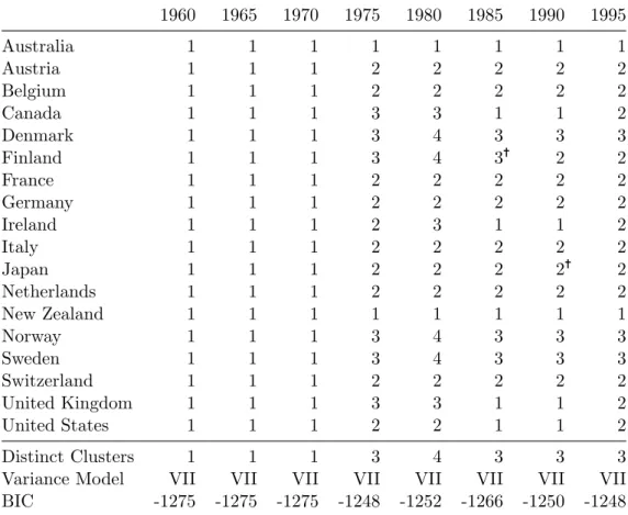
cluster in 1970.
By 1975, there are signs of three worlds emerging, but it is not until 1980 that the countries are properly classified by conventional standards. For the 1975 interval, measure set A once again contains only two clusters, with Australia and New Zealand categorized as a discrete cluster. When the analysis is extended to the measure set B, however, the Nordic countries, Canada, and the United Kingdom break off to form a third cluster (see Table 15). The inclusion of the second measure of defamilialization, the parental leave replacement rate, causes this third cluster to split into two, with Canada and the United Kingdom joined by Ireland and the United States in one group and the Nordic countries minus Norway in the other. Moving forward to 1980, three clusters are secerned in measure set A, with the Anglo-Saxon countries divided among two clusters and the remaining 12 countries and the United States assigned to the third cluster. Looking at the results for measure sets B and C, the addition of the measures for the public provision of social services and defamilialization again helps differentiate the Nordic countries, leading to a fourth cluster. Finally, as Table 12 shows, the inclusion of measures for post-tax/transfer poverty and activation produces clustering that corre-sponds exactly with the conventional three-world typology: Austria, Belgium, France, Germany, Italy, Japan, the Netherlands, and Switzerland belonging to the conservative regime; Australia, Canada, Ireland, the United Kingdom, and the United States com-prising the liberal regime; and Denmark, Finland, Norway, and Sweden making up the social democratic regime.(e.g., see Esping-Andersen and Hicks 2005).
Looking beyond the cluster numbers and country categorizations, the geometry and certainty reported for each iteration of the analysis are quite consistent across measure sets and intervals. According the model-selection output, the optimal parameterization of the covariance matrix for nearly every model is one based on a spherical distribu-tion. The clusters generated by this parameterization feature variable volumes but equal shapes. At the same time, the results indicate a high degree of certainty in the classifi-cation of countries, with uncertainty levels for all classificlassifi-cations below the conventional threshold of 0.05 and most below 0.001.
Turning to the results from agglomerative hierarchical cluster analyses, the dendro-grams generally confirm the findings from the model-based approach. In the 1950s, the dendrograms show Australia and New Zealand to be distinctly separated from the re-maining 16 countries. For 1975, the dendrogram for measure set B depicts a tree that exactly corroborates the three clusters found by the accompanying model-based analysis with the one exception of Ireland. There are also direct correspondences between all of the dendrograms and model-based results for all of the measure sets for 1980 and 1985. For the intervals that the model-based approach did not find any distinct clusters, the corresponding dendrograms reveal some tentative clusters. In 1960, the dendrogram for measure set B suggests that Anglo-Saxon countries, Nordic countries, and France formed one large group and the remaining continental European countries and Japan formed another. However, the AU p-values for these two large clusters—78% and 69%— are relatively low, so the clusters should be seen as indeterminate. For 1965, these two clusters are again identified and with higher certainty, 87% and 88%, respectively. By 1970, however, the dendrograms for measure sets B and C intimate that the Nordic countries had become grouped with the continental European countries and Japan, leaving the Anglo-Saxon countries clustered together. The p-values for the clusters in the first of these dendrograms are weak, but the ones reported for the second are stronger: 86% and 82%.
Discussion and Conclusions
findings suggest that Esping-Andersen made a fortunate decision in selecting 1980 as the year for his cross-sectional analysis that engendered the three-world typology. Look-ing more closely at the results, however, this study casts further doubt on the validity of Esping-Andersen’s original approach to identifying real-world welfare-state clusters. Analysis of measure set A, which closely approximates the data used by Esping-Andersen in his analysis, did discern three clusters in 1980, but the memberships of these clusters in no way resemble those of Esping-Andersen’s groupings. In essence, the results from this analysis add further weight to Esping-Andersen’s key findings, but they again bring into question the approach he used to generate these findings.
In addition, this study confirms that the public provision of social services and defa-milialization are essential in differentiating between the three worlds of welfare. Looking at 1975, for instance, three worlds are established only after including a measure for each of these two dimensions, as implied by the analysis of measure set B. This effect is fur-ther evident in the results reported for each interval from 1980 up through 1995, where there is shift in distinct clusters from two for measure set A to three for measure set B. As theorized, the dimensions for the public provision of social services and defamil-ialization appear to be especially crucial in distinguishing between the conservative and social democratic welfare state regimes. These results also imply that decommodifica-tion and stratificadecommodifica-tion alone are insufficient for distinguishing between contemporary welfare state regimes, a finding that conflicts with the results of prior replication work on Esping-Andersen’s three-worlds typology using cluster analysis (Edwards 2003).26
There also appears to be some support from this study for the notion that the Aus-tralia and New Zealand welfare states should be considered distinct from their Anglo-Saxon cousins. In the 1950s, Australia and New Zealand are assigned to their own cluster, which squares with Hicks’ claim that these two countries were early welfare con-solidators (1999). After the 1950s, however, Australia and New Zealand went from being two of the most advanced welfare states in the world to being two major welfare-state laggards. The lack of any distinct clusters during the 1960s supports this point because it denotes that the other welfare states caught up with Australia and New Zealand, erasing the relative leads of these two countries. By 1975, Australia and New Zealand
26
do again emerge as a relatively distinct group, but at this point they are distinguished by their poor and restricted systems of entitlements, not high levels of welfare state gen-erosity. Moving on to the 1980s, however, Australia and New Zealand are less distinctive from the other Anglo-Saxon countries, presumably because retrenchment helped spur convergence towards a more uniform liberal model in these countries. Overall, their appears to be some justification for considering Australia and New Zealand as members of a separate “Antipodean” or “wage earner” welfare state regime, particularly for years prior to 1980.
The emergence of three worlds in the 1975 to 1985 period is consistent with the the-ory that welfare state development in the postwar era was largely a function of long-term partisan composition of government. According to this theory, the relative strength of different political forces over time determined the trajectories of welfare states in ad-vanced capitalist countries after World War II (Huber and Stephens 2001). Where social democratic and Christian democratic political forces were dominant, welfare states be-came more generous and comprehensive over time, though with some notable divergences in their social-policy designs. In contrast, the continued ascendency of secular center and right-wing political forces in other countries propagated more minimal or residual welfare states over time. When examining the results from this study, the composition of the three worlds discerned in 1980 for measure set D reflect well-known trends in par-tisan political incumbency. The Nordic countries, which all had strong social democratic parties in the decades after World War II, are exclusively grouped together while the continental European countries, which were dominated by Christian democratic forces in this postwar period, are also clustered together. Moreover, the Anglo-Saxon countries, which had strong centrist or right-wing tendencies in the decades after World War II, are members of a single cluster. As alluded to before, Australia and New Zealand may represent more extreme cases of how the prolonged control of government by right-wing political forces can impel welfare states to become more residual in nature.
post-war period. The cluster analyses for the 1950s indicate that most welfare states were indistinguishable from one another, with the exception of the Antipodean countries. Even during the Golden Age of the 1960s and 1970s, welfare states remained relatively similar to one another, probably because nearly all welfare states were undergoing ex-pansion at this time. The dendrograms for this period, however, suggest that subtle shifts were occurring beneath the surface, with the Anglo-Saxon and Nordic countries bifurcating into separate groups and the latter of these two groups merging together with the group of continental European countries and Japan. By the mid-1970s, however, the Nordic countries split off into their own distinct cluster, which is just about the point when women’s mobilization started to drive a new expansion of public services in these countries. Therefore, while welfare expansion was leveling off in the Anglo-Saxon and continental European states in the early to mid-1970s, it was accelerating in the Nordic countries, helping to establish a distinct social democratic welfare model.
Once the three worlds emerged around 1980, there is evidence that they remained relatively stable, a finding that is congruous with the notion of path dependence. As mentioned before, the concept of path dependence holds that institutions become self-reinforcing over time because the costs of reversals or switching to alternatives increase over time (Pierson 2000). As the results from this study show, countries generally became locked into the three worlds once these worlds became pronounced. For instance, once the social democratic regime surfaced between 1975 and 1980, the Nordic countries were consistently tied to this regime type. Of course, Belgium, Canada, and Finland do switch regimes at some points during the 1980–1995 period, so a strict form of path dependence is not justified in explaining the persistence of the three worlds.
interpretation of welfare state development.
APPENDIX
Table 1: Rank-Order of Welfare States in Terms of Combined Decommodification, 1980
Country Decommodificaton Score
Australia 13.0
United States 13.8
New Zealand 17.1
Canada 22.0
Ireland 23.3
United Kingdom 23.4
Italy 24.1
Japan 27.1
France 27.5
Germany 27.7
Finland 29.2
Switzerland 29.8
Austria 31.1
Belgium 32.4
Netherlands 32.4
Denmark 38.1
Norway 38.3
Sweden 39.1
Mean 27.2
S.D. 7.7
Table 2: Clustering of Welfare States According to Liberal, Conservative, and Socialist Regime Attributes, 1980
Liberalism Conservatism Socialism
Strong Australia (10) Austria (8) Denmark (8)
Canada (12) Belgium (8) Finland (6)
Japan (10) France (8) Netherlands (6)
Switzerland (12) Germany (8) Norway (8)
United States (12) Italy (8) Sweden (8)
Medium Denmark (6) Finland (6) Australia (4)
France (8) Ireland (4) Belgium (4)
Germany (6) Japan (4) Canada (4)
Italy (6) Netherlands (4) Germany (4)
Netherlands (8) Norway (4) New Zealand (4)
United Kingdom (6) Switzerland (4)
United Kingdom (4)
Low Austria (4) Australia (0) Austria (2)
Belgium (4) Canada (2) France (2)
Finland (4) Denmark (2) Ireland (2)
Ireland (2) New Zealand (2) Italy (0)
New Zealand (2) Sweden (0) Japan (2)
Norway (0) Switzerland (0) United States (0)
Sweden (0) United Kingdom (0)
United States (0) Source: Esping-Andersen 1990, 74, Table 3.3.
Table 3: Core Dimensions of the Three Welfare State Regimes Dimension Liberal Conservative Social Democratic
Decommodification low medium high
Public provision of social services
low low high
Population coverage selective occupational universal
Income redistribution low low high
Post-tax/transfer poverty
low medium high
Defamilialization low low high
Activation medium low high
Table 4: Welfare State Clusters for 1952 and 1980
1952a 1980b
Consolidators Social Democratic
Austria Austria
Australia Belgium
Belgium Denmark
Denmark Netherlands
Netherlands Norway
New Zealand Sweden
Norway
Sweden Conservative
United Kingdom Finland
France
Non-Consolidators Germany
Canada Italy
Finland Japan
France Switzerland
Germany
Italy Liberal
Japan Australia
Switzerland Canada
United States Ireland
New Zealand United Kingdom United States
aIreland is excluded from Hicks’ pre-Wold War II analysis for
“excessively mimicking British social policy” (1999, 31). At one point, however, Hicks does imply that Ireland was in fact a consolidator in 1952 (1999, 111).
bBased on Esping-Andersen’s decommodification clusters.
Table 5: Measure Descriptions and Sources
Measure Description Source
Decommodification
Old-Age Pensions
Minimum net RR Net minimum annual replacement rate for old-age pensions for a single worker.
SCIP (2007) APW net RR Net annual replacement rate for old-age
pensions for a single APW.
SCIP (2007) Contribution period Number of years of contribution
required to qualify for benefit, made in course of the reference period.
SCIP (2007)
Financed by Insured Total proportion of insurance fund receipts derived from contributions by the individuals insured.
SCIP (2007)
Sick Pay
APW net RR Net replacement rate for a single APW for a 26-week sickness spell, with the prior half-years wage income excluded.
SCIP (2007)
Waiting Days Number of legislated administrative waiting days at the beginning of a sickness spell, during which no benefits are paid out.
SCIP (2007)
Duration Number of weeks for which the sickness benefit is payable to a single industrial worker with a work record.
SCIP (2007)
Contribution period Number of weeks of contribution required to qualify for benefit, made in course of the reference period.
SCIP (2007)
Unemployment Insurance
APW net RR Net replacement rate for a single APW for a 26-week unemployment spell, with the prior half-years wage income
excluded.
SCIP (2007)
Waiting Days Number of legislated administrative waiting days at the beginning of a unemployment spell, during which no benefits are paid out.
SCIP (2007)
Duration Number of weeks for which the unemployment benefit is payable to a single industrial worker with a work record.
SCIP (2007)
Contribution period Number of weeks of contribution required to qualify for benefit, made in course of the reference period.
Table 5: Measure Descriptions and Sources (continued)
Measure Description Source
Public Provision of Social Services
Government Employment
Civilian government employment as a percentage of the working-age
population.
CWS (2004)
Population Coverage Pension Take-Up Rate
Share of the population above the normal pension age that is receiving a pension.
SCIP (2007)
Pension Coverage Rate
Percentage of the population aged 15–65 that will be eligible for pensions at the normal age of retirement.
SCIP (2007)
Sickness Coverage Rate
Percentage of labor force that is covered by sickness insurance.
SCIP (2007) Unemployment
Coverage Rate
Percentage of labor force that is covered by unemployment insurance.
SCIP (2007)
Public Share of Health Spending
Public share of total spending on health care as a percentage of GDP.
CWS (2004) Income Redistribution
Pension Benefit Equality
Net annual replacement rate for old-age pensions for a single APW as a
percentage of the stipulated maximum net replacement rate.
SCIP (2007)
Sickness Benefit Equality
Net annual replacement rate for sick pay for a single APW as a percentage of the stipulated maximum net replacement rate.
SCIP (2007)
Unemployment Benefit Equality
Net annual replacement rate for unemployment insurance for a single APW as a percentage of the stipulated maximum net replacement rate.
SCIP (2007)
Gini Index – Gross Estimated Gini index of gross disposable household income.
SCIP (2007) Gini Index – Net Estimated Gini index of net disposable
household income.
SCIP (2007)
Post-Tax/Transfer Poverty
Relative Poverty – Total
Percentage of households with disposable incomes below 50% of the average disposable household income.
LIS (2009)
Table 5: Measure Descriptions and Sources (continued)
Measure Description Source
Post-Tax/Transfer Poverty (cont.)
Relative Poverty – Children
Percentage of children in households with disposable incomes below 50% of the average disposable household income.
LIS (2009)
Relative Poverty – Elderly
Percentage of elderly households with disposable incomes below 50% of the average disposable household income.
LIS (2009)
Defamilialization Female Labor Force Participation
Percentage of women aged 15–64 who are in the labor force.
CWS (2004) Parental Leave RR Average replacement rate for parental
leave for a 52-week period.
Gauthier and Bortnik (2001) Activation
Active Labor Market Policies
Total public spending on active labor market policies as a percentage of GDP divided by the unemployment rate.
SOCX (2008)
Table 6: Sets of Measures Set
Dimension A B C D
Decommodification 12 12 12 12 Public provision of
social services
1 1 1
Population coverage 4a 5 5 5 Income redistribution 3b 5 5 5
Post-tax/transfer poverty
3
Defamilialization 1c 2 2
Activation 1
Total Variables 19 24 25 29
a3 coverage rates and take-up rate. b3 benefit-equality measures.
Table 7: Possible Parameterizations of the Covariance matrix Σkand Their Geometric Features
Identifier Model Distribution Volume Shape Orientation
EII λI spherical equal equal NA
VII λkI spherical variable equal NA
EEI λA diagonal equal equal along the axes
VEI λkA diagonal variable equal along the axes
EVI λAk diagonal equal variable along the axes
VVI λkAk diagonal variable variable along the axes
EEE λDADT ellipsoidal equal equal equal
EEV λDkADTk ellipsoidal equal equal variable VEV λkDkADTk ellipsoidal variable equal variable VVV λkDkAkDkT ellipsoidal variable variable variable
Source: Fraley and Raftery 2007b, 6, Table 1
Table 8: Number of Distinct Clusters Detected For Each Set of Measures
Set of Measures
Year A B C D
1950 2
1955 2
1960 4 1
1965 1 1
1970 2 1 1
1975 2 3 4
1980 3 4 4 3
1985 2 3 3 3
1990 2 3 3 3
Table 9: Country Classifications for Measure Set A for Each Five-Year Interval from 1950– 1995
1950 1955 1960 1965 1970 1975 1980 1985 1990 1995
Australia 1 1 1 1 1 1 1 1 1 1
Austria 2 2 2 1 2 2 2 2 2 2
Belgium 2 2 2 1 2 2 2 2 2 2
Canada 2 2 3 1 2 2 3 1 2 2
Denmark 2 2 3 1 2 2 2 2= 2 2
Finland 2 2 3 1 2 2 2 2 2 2
France 2 2 2 1 2 2 2 2 2 2
Germany 2 2 2 1 2 2 2 2 2 2
Ireland 2 2 4 1 2 2 3 1 2 1
Italy 2 2 2 1 2 2 2 2< 2 2
Japan 2 2 2 1 2 2 2 2= 2 2
Netherlands 2 2 3< 1 2 2 2 2 2 2
New Zealand 1 1 1 1 1 1 1 1 1 1
Norway 2 2 3 1 2 2 2 2 2 2
Sweden 2 2 3 1 2 2 2 2 2 2
Switzerland 2 2 3 1 2 2 2 2 2 2
United Kingdom 2 2 4 1 2 2 3 1 2 2
United States 2 2 3 1 2 2 2 1 2 2
Distinct Clusters 2 2 4 1 2 2 3 2 2 2
Variance Model VII VII VII VII VII VII VII VII VII EII
BIC -1010 -1006 -1009 -1010 -997 -976 -992 -995 -982 -982
Table 10: Country Classifications for Measure Set B for Each Five-Year Interval from 1960–1995
1960 1965 1970 1975 1980 1985 1990 1995
Australia 1 1 1 1 1 1 1 1
Austria 1 1 1 2 2 2 2 2
Belgium 1 1 1 2 2 2 2 2
Canada 1 1 1 3 3 1 1 2
Denmark 1 1 1 3 4 3 3 3
Finland 1 1 1 3 4 3= 2 2
France 1 1 1 2 2 2 2 2
Germany 1 1 1 2 2 2 2 2
Ireland 1 1 1 2 3 1 1 2
Italy 1 1 1 2 2 2 2 2
Japan 1 1 1 2 2 2 2= 2
Netherlands 1 1 1 2 2 2 2 2
New Zealand 1 1 1 1 1 1 1 1
Norway 1 1 1 3 4 3 3 3
Sweden 1 1 1 3 4 3 3 3
Switzerland 1 1 1 2 2 2 2 2
United Kingdom 1 1 1 3 3 1 1 2
United States 1 1 1 2 2 1 1 2
Distinct Clusters 1 1 1 3 4 3 3 3
Variance Model VII VII VII VII VII VII VII VII
Table 11: Country Classifications for Measure Set C for Each Five-Year Interval from 1970–1995
1970 1975 1980 1985 1990 1995
Australia 1 1 1 1 1 1
Austria 1 2 2 2 2 2
Belgium 1 2 2 2 2 2
Canada 1 3 3 1 2 2
Denmark 1 4 4 3 3 3
Finland 1 4 4 3 3 2
France 1 2 2 2 2 2
Germany 1 2 2 2 2 2
Ireland 1 3 3 1 2 2
Italy 1 2 2 2 2 2
Japan 1 2 2 2 2 2
Netherlands 1 2 2 2 2 2
New Zealand 1 1 1 1 1 1
Norway 1 2= 4 3 3 3
Sweden 1 4 4 3 3 3
Switzerland 1 2 2 2 2 2
United Kingdom 1 3 3 1 2 2
United States 1 3 2 1 2 2
Distinct Clusters 1 4 4 3 3 3
Variance Model VII VII VII VII VII VII
BIC -1328 -1322 -1299 -1308 -1298 -1292
Table 12: Country Classifications for Measure Set D for Each Five-Year Interval from 1980–1995
1980 1985 1990 1995
Australia 1 1 1 1
Austria 2 2 2 2
Belgium 2 3 2 2
Canada 1 1 1 2<
Denmark 3 3 3 3
Finland 3 3 3 2
France 2 2 2 2
Germany 2 2 2 2
Ireland 1 1 1 1
Italy 2 2 2 2
Japan 2 2 2 2
Netherlands 2 2 2 2
New Zealand 1 1 1 1
Norway 3 3 3 3
Sweden 3 3 3 3
Switzerland 2 2 2 2
United Kingdom 1 1 1 1
United States 1 1 1 1
Distinct Clusters 3 3 3 3
Variance Model VII VII VII VII
BIC -1522 -1523 -1502 -1488
Table 13: Country Clusters for Measure Set A for Each Five-Year Interval from 1950– 1995
1950 1955 1960 1965 1970
Austria Austria Austria Australia Austria Belgium Belgium Belgium Austria Belgium Canada Canada France Belgium Canada Denmark Denmark Germany Canada Denmark Finland Finland Italy Denmark Finland France France Japan Finland France
Germany Germany France Germany
Ireland Ireland Canada Germany Ireland Italy Italy Denmark Ireland Italy
Japan Japan Finland Italy Japan
Netherlands Netherlands Netherlands Japan Netherlands Norway Norway Norway Netherlands Norway Sweden Sweden Sweden New Zealand Sweden Switzerland Switzerland Switzerland Norway Switzerland United Kingdom United Kingdom United States Sweden United Kingdom United States United States Switzerland United States
Ireland United Kingdom
Australia Australia United Kingdom United States Australia New Zealand New Zealand New Zealand
Australia New Zealand
1975 1980 1985 1990 1995
Austria Austria Austria Austria Austria Belgium Belgium Belgium Belgium Belgium Canada Denmark Denmark Canada Canada Denmark Finland Finland Denmark Denmark Finland France France Finland Finland France Germany Germany France France Germany Italy Italy Germany Germany Ireland Japan Japan Ireland Italy Italy Netherlands Netherlands Italy Japan Japan Norway Norway Japan Netherlands Netherlands Sweden Sweden Netherlands Norway Norway Switzerland Switzerland Norway Sweden Sweden United States Sweden Switzerland Switzerland Australia Switzerland United Kingdom United Kingdom Canada Canada United Kingdom United States United States Ireland Ireland United States
United Kingdom New Zealand Australia Australia United Kingdom Australia Ireland New Zealand Australia United States New Zealand New Zealand