He_unc_0153M_17076.pdf

(1)

SPEEDED3PL MODELS WITH ITEM ORDER EFFECTS AND INDIVIDUAL DIFFERENCES IN TOLERANCE FOR DIFFICULTY

Jason He

A dissertation submitted to the faculty of the University of North Carolina at Chapel Hill in partial fulfillment of the requirements for the degree of Doctor of Philosophy in the

Department of Psychology and Neuroscience.

Chapel Hill 2017

(2)

c

2017

Jason He

(3)

ABSTRACT

JASON HE: Speeded 3PLmodels with item order effects and individual differences in

tolerance for difficulty.

(Under the direction of David Thissen)

(4)

(5)

ACKNOWLEDGMENTS

(6)

TABLE OF CONTENTS

LIST OF TABLES . . . viii

LIST OF FIGURES . . . viii

1 INTRODUCTION . . . 1

1.1 What isspeededness? . . . 1

1.1.1 Local independence and multidimensionality . . . 2

1.2 Prior art . . . 3

1.2.1 ‘Hybrid’ and mixture models . . . 3

1.2.2 ‘Gradual process change’ . . . 3

1.2.3 ‘Leave the harder till later’ . . . 6

2 MODELS AND METHODS OF COMPUTATION . . . 11

2.1 ‘Full’ specification . . . 11

2.2 Parameter estimation . . . 13

2.2.1 Expectation–Maximization (EM) . . . 15

2.2.2 Metropolis–Hastings Robbins–Monro (MH–RM) . . . 17

2.2.3 Derivatives used in the optimization steps . . . 19

2.2.4 Estimation of population means and covariances . . . 20

2.3 The empirical data . . . 21

2.4 Research objectives . . . 21

(7)

3.1 Comments on the algorithms . . . 23

3.1.1 MH–RM algorithm . . . 23

3.1.2 EM algorithm . . . 23

3.2 Simulation estimates . . . 24

3.3 Empirical example . . . 30

4 DISCUSSION . . . 43

4.1 Substantive interpretations . . . 43

4.2 Research limitations . . . 44

4.3 Implications for practitioners . . . 44

4.4 Future directions for research . . . 45

APPENDIX A EMPIRICAL VARIANCE–COVARIANCE MATRICES . . . 47

APPENDIX B ANALYTICAL GRADIENT . . . 51

APPENDIX C R SYNTAX . . . 53

(8)

LIST OF TABLES

2.1 The population mean of each latent variable used to generate simulated data. . . 22

2.2 Latent variable variances and covariances used to generate simulated data. . . 22

3.1 Recovery of population parameters simulated from and fitted with the full model. . 24

3.2 Recovery of item parameters simulated from the full model, fitted to various models. 26 3.3 −2 log likelihood values from data simulated from and fit to various models. . . . 30

3.4 Akaike’s information criteria from data simulated from and fit to various models. . 30

3.5 Bayesian information criteria from data simulated from and fit to various models. . 31

3.6 Fit indices from each replication of the first of five empirical test forms. . . 37

3.7 Fit indices from each replication of the second of five empirical test forms. . . 37

3.8 Fit indices from each replication of the third of five empirical test forms. . . 38

3.9 Fit indices from each replication of the fourth of five empirical test forms. . . 38

3.10 Fit indices from each replication of the fifth of five empirical test forms. . . 39

3.11 Summary statistics of item parameters from various speeded models relative to 3PLparameters from the original calibration. . . 39

3.12 Mean values of each latent variable in the full model in the population. . . 40

3.13 Variance–covariance matrices, averaged over replications, involving each latent variable in the full model in the population. . . 40

3.14 Mean values of each latent variable in the Goegebeur et al. (2008) model in the population. . . 41

3.15 Variance–covariance matrices, averaged over replications, involving each latent variable in the Goegebeur et al. (2008) model in the population. . . 41

3.16 Mean values of theτ latent variable in the Chang et al. (2014) model in the popu-lation. . . 41

3.17 Variance–covariance matrices, averaged over replications, for the Chang et al. (2014) model in the population. . . 42

(9)

A.2 Covariance matrices from each replication of data fit with the Goegebeur et al. (2008) model. . . 49 A.3 Covariance matrices from each replication of data fit with the Chang et al. (2014)

(10)

LIST OF FIGURES

1.1 The multiplierminh1, 1− i I +η

λi

as a function of_Ii, the position of an item as

a proportion of test length. . . 5

1.2 Goegebeur, De Boeck, Wollack, & Cohen (2008) . . . 7

1.3 The multiplier exp [−s(bi−τ)·1(bi > τ)] as a function of b for four different combinations ofsandτ. . . 8

1.4 The Chang et al. (2014) model for itemias a decision tree. . . 9

2.1 The full model as a decision tree. . . 12

2.2 Effects of various values ofs. . . 14

3.1 Recovery of item parameters simulated from the full model, fitted with the full model. . . 25

3.2 Recovery of item parameters simulated from the full model, fitted to the Goegebeur et al. (2008) model. . . 27

3.3 Recovery of item parameters simulated from the full model, fitted to the Chang et al. (2008) model. . . 28

3.4 Recovery of item parameters simulated from the full model, fitted to the 3PL model. 29 3.5 Item parameter estimates from the Full model vs. 3PL values. . . 34

3.6 Item parameter estimates from the Goegebeur et al. (2008) model vs. 3PL values. . 35

(11)

1 INTRODUCTION 1.1 What isspeededness?

Speededness occurs in any power test1 _{when time constraints interfere with the item}

re-sponse process. Affected examinees may omit items, guess at random, or otherwise underrep-resent their ability on some items as a consequence of pressure to finish within a time limit. Future examinees may also be affected through the biasing effects of speeded responses on test calibration and equating.

Traditional models in item response theory (IRT) neglect speededness, and the model-based literature on the phenomenon remains sparse. In this manuscript, I survey the nascent work on IRT models for speededness, and develop a model to accommodate a broad range of test-taking strategies. I study the performance of the model with simulated data and an application to empirical test data, considering two algorithms for the estimation of model parameters.

The standard IRT framework involves a vector of binary responses Y0 = {Y1, Y2, . . . , YI}

for a test ofI items. The three-parameter logistic (3PL) model, common for multiple-choice tests with guessing, specifies that an examinee of ability θ responds correctly (Yi = 1) with probability

P ≡Pr(Yi = 1|θ) =gi+

1−gi

1 + exp [−ai(θ−bi)]

(1.1)

and incorrectly withPr(Yi = 0)≡1−P. Under this model, a correct response is a function of one random effect, an examinee-specific variableθ, usually ability, and three fixed parameters: ai ∈[0,∞), the power of an item to discriminate between examinees at lower and higher levels of proficiency; bi ∈ (−∞,∞), item difficulty; andgi ∈ [0,1], a lower asymptote parameter interpreted loosely to represent guessing. If gi = 0 for all items, the model reduces to a 1_{A power test is distinguished from a speed test, which measures only the rate at which examinees perform}

(12)

two-parameter logistic (2PL); if, furthermore, ai = a for all items, the model reduces to a one-parameter logistic (1PL).

IRT assumes local independence such that, conditional on the value of θ, the correct or incorrect response of an examinee to itemihas no effect on the response of the same examinee to itemj for any pair of itemsi 6= j. The likelihood function for any vector of responsesY, givenθ, is

L=Y i

PYi

i (1−Pi)1−Yi. (1.2)

1.1.1 Local independence and multidimensionality

Local independence defines the latent variable and is therefore fundamental to IRT. Items that are locallydependentmay introduce bias in estimates of fixed and random effects and their standard errors. Testlets2_{, redundancy in the items, and test speededness may all produce local}

dependence (Chen & Thissen, 1997), but psychometricians have observed that speededness is routinely overlooked even on educational tests where it would be of particular concern (Lu & Sireci, 2007).

The goal of most educational tests is to measure ability, but if individual differences in speed and ability are distinct (if correlated) factors, then they must constitute at least two latent dimensions. A unidimensional model wherein θ is ability, as it is in Equation 1.1, cannot account for all dependencies between responses if speed relates to the probability of responding correctly.

(13)

items that exhibit differential item functioning. 1.2 Prior art

1.2.1 ‘Hybrid’ and mixture models

Even as the consequences of speededness have been widely recognized, the model-based literature remains sparse. In one early foray, Yamamoto (1982) used IRT with latent class analysis in what he termed a “hybrid” model and explored its application to test speededness. Yamamoto and Everson (1997) subsequently described a mixture of examinees whose item re-sponses are characterized by either a 2PL response function or by random guessing; the model incorporated IRT parameters for items and abilites in addition to parameters that described the distribution of examinees who would switch from 2PL responding to random guessing.

Also within a latent class framework, but with a 1PL item response function, Bolt, Cohen, & Wollack (2002) imposed ordinal constraints on item difficulty to distinguish two classes (1 and 2) of examinees who respectively are and are not affected by speededness. The difficulty parameters were constrained to be equal between classes for items that appeared early in a test, and constrained to be higher in Class 1 than in Class 2 for items thereafter. Parameter estimates from the speededness-unaffected Class 2 were deemed unbiased estimates of item difficulty. A 3PL analog to this model was developed one year later (Bolt, Mroch, & Kim, 2003).

The basic concepts that examinees guess at random when speeded, and that speededness manifests on items ordered toward the end of a test, have been refined in more contemporary models, two of which form the basis of the model to be described in Chapter 2.

1.2.2 ‘Gradual process change’

A model described by Goegebeur et al. (2008) carries the spirit of Yamamoto’s (1982) model without the backdrop of latent classes. The Goegebeur et al. (2008) model of “grad-ual process change” comprises two stochastic processes: (1) problem solvingand (2)random guessing. The model specifies that all examinees answer questions in the same order,

(14)

gradually from problem solving, hence the model’s nickname. Gradations within the process change are controlled by an examinee-specific decay rate λ. Thus, while the canonical 3PL model contains only one random effect, the Goegebeur et al. (2008) model contains three: θ (ability);η(change point); andλ(decay rate).

For a test of itemsi= 1, . . . , I, the Goegebeur et al. (2008) model is

Pr(Yi = 1 |θ, η, λ) = gi+

1−gi

·min

"

1,

1− i

I +η

λ#

(1.3)

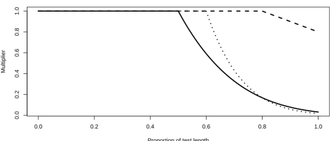
where η ∈ [0,1] is a proportion of test length that determines the item number at which an examinee begins speeding. If a test containsI = 50 items, thenη = 0.8 correponds to item i = 40 such that items 1–39 are unaffected by speeding. Equivalently, if η = 0.8 for all examinees and the test comprised only the first 39 items, then the Goegebeur et al. (2008) model is identical to a canonical 3PL model. Subsequent items (i≥40), however, are affected with increasing severity, at a rate controlled byλ∈[0,∞). The model implied probability of a correct response to those final 10 items (i= 40,41, . . . ,50) equals a 3PL probability multiplied by(1−(i/50) +η)λ_{. The magnitude of this multiplier—a decay function—decreases at a rate} controlled byλ; see Figure 1.1.

By nature of gradualprocess change, controlled byλ, the Goegebeur et al. (2008) model is an improvement on the Yamamoto & Everson (1997) hybrid model which specified that examinees, once speeded, switch immediately to random guessing. Further, because of its examinee-varying change points,η, the Goegebeur et al. (2008) model is an extension of earlier mixture model approaches in which the change point is a fixed parameter (Bolt et al., 2002, 2003).

To see how the Goegebeur et al. (2008) model comprises two stochastic processes, denote the decay function plotted in Figure 1.1

Λ = min

"

1,

1− i

I +η

λ#

(15)

0.0 0.2 0.4 0.6 0.8 1.0

0.0

0.2

0.4

0.6

0.8

1.0

Goegebeur et al. (2008) multiplier by item position

Proportion of test length

Multiplier

Figure 1.1: The multiplierminh1, 1− i I +η

λi

as a function of _Ii, the position of an item as a proportion of test length.

(16)

An examinee who approaches itemiwill respond with a problem solving process with prob-ability Λ or a random guessing process with probability 1−Λ. Under problem solving, the examinee knows the answer with probability

K = 1

. (1.5)

If the examinee does not know the answer, the examinee guesses at random. Under random guessing, the probability of a correct response isgi. Therefore,

Pr(Yi = 1|θ, η, λ) = ΛK+ Λ(1−K)gi+ (1−Λ)gi (1.6)

=gi+ ΛK(1−gi); (1.7)

the right hand side expands to become

gi+ 1−gi

·min

"

1,

1− i

I +η

λ#

, (1.8)

exactly as before, in Equation 1.3. This two-stage procedure is illustrated in Figure 1.2. 1.2.3 ‘Leave the harder till later’

(17)

itemi

late; guess

0 1

g 1−g

early; solve

don’t know; guess

0 1

g 1−g

1

K 1−K

Λ 1−Λ

Figure 1.2: The Goegebeur et al. (2008) model for itemias a decision tree. Edge labels are probabilities. A correct response is 1 ; an incorrect response is 0 .

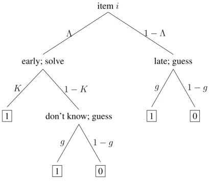
Like Goegebeur et al. (2008), Chang et al. (2014) expand a traditional IRT model with a multiplier, the effects of which are plotted in Figure 1.3. The two new parameters areτ, the aforementioned examinee-specific threshold, ands, a fixed, global rate of test speededness. A 2PL model is used in place of the 3PL; equivalently,gi = 0for all items. In compact form, the Chang et al. (2014) model is

Pr(Yi = 1|θ, τ) =

1

1 + exp [−ai(θ−bi)]·exp [−s(bi−τ)·1(b > τ)] (1.9)

where 1 is the binary indicator function and s is a fixed parameter, like all other variables denoted by Roman letters, but does not vary over items (and thus carries no subscript; n.b. the latent variables vary over examinees but are not subscripted throughout this manuscript).

(18)

−3 −2 −1 0 1 2 3

0.0

0.2

0.4

0.6

0.8

1.0

Chang et al. (2014) multiplier by item difficulty

Difficulty

Multiplier

Figure 1.3: The multiplier exp [−s(bi−τ)·1(bi > τ)] as a function of b for four different combinations ofsandτ.

(19)

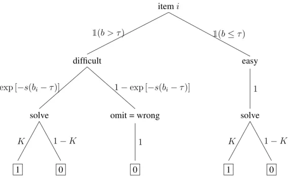
itemi

easy

solve

0 1

K 1−K

1 difficult

omit = wrong

0 1 solve

0 1

K 1−K

exp [−s(bi−τ)] 1−exp [−s(bi−τ)]

1(b > τ) ₁₍_b_≤_τ₎

Figure 1.4: The Chang et al. (2014) model for itemias a decision tree.

Ifiis attempted immediately (bi ≤τ) then

Yi,immediate ∼Bernoulli

1

. (1.10)

Ifiis deferred (branching left on the decision tree), the examinee will return to it with proba-bilityexp [−si(bi−τ)], so that

Yi,deferred ∼Bernoulli

exp [−si(bi−τ)] 1 + exp [−ai(θ−bi)]

. (1.11)

If the examinee omits itemi, thenYi = 0.

Although the Goegebeur et al. (2008) model can also be described as a two-step process involving problem solving and random guessing (see Figure 1,2), the underlying mechanism of speededness is distinct. Whereas Goegebeur et al. (2008) emphasized item order, Chang et al. (2014) emphasize item difficulty.

(20)

constraint used by Goegebeur et al. (2008) that examinees must answer items in one partic-ular order. While it models a scenario in which examinees may skip around a test, Chang et al. (2014) does not include a model for guessing. Further, no distinction is made between items an examinee attempts, but answers incorrectly, and items an examinee must omit, due to speededness.

(21)

2 MODELS AND METHODS OF COMPUTATION

A straightforward combination of the Goegebeur et al. (2008) and Chang et al. (2014) models yields a “full” model of the effects of item order and item difficulty.

2.1 ‘Full’ specification

With four latent variables, all as previously defined,

Pr(Yi = 1|θ, η, λ, τ) =gi+ 1−gi

·min

"

1,

1− i

I +η

λ#

·exp

−1

2(bi−τ)·1(b > τ)

| {z }

see Figure 2.1

(2.1)

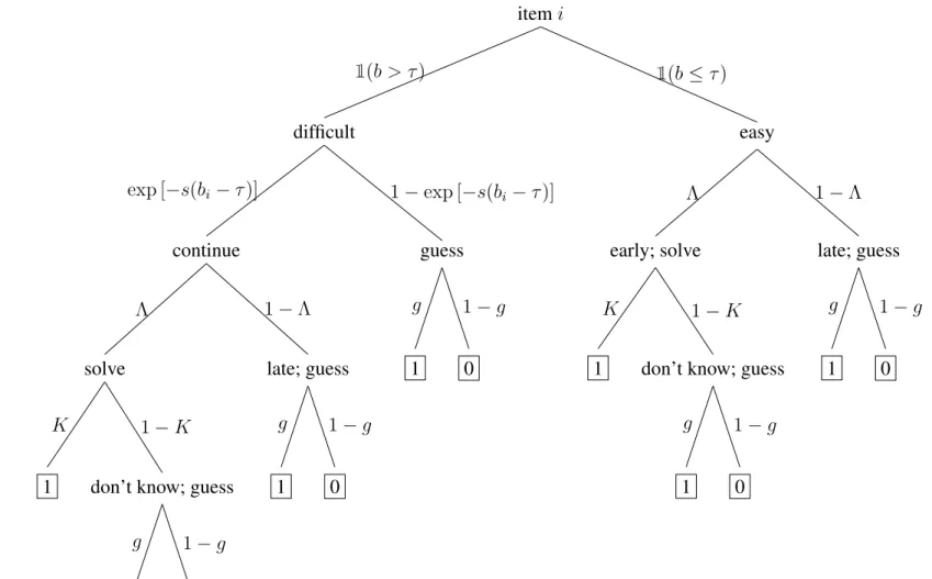
andPr(Yi = 0 | θ, η, λ, τ) = 1−Pr(Yi = 1 | θ, η, λ, τ).This model accounts for item order as well as an examinee-specific tolerance for difficulty in constructing a decaying 3PL item response function, and should therefore describe the behavior of an examinee who answers easier items first and saves the difficult items for last, but otherwise follows the general order of the test. (That is, the examinee does not purposefully randomize the order of items or work through the test booklet from back to front.) As such, the effect of item order remains salient; as suggested by Goegebeur et al. (2008), an examinee should be less likely to solve an item at the end of a test. The part of the model due to Chang et al. (2014) implies that an examinee is less likely to solve an item if it is difficult. A decision tree representation of the full model is in Figure 2.1.

(22)

itemi

easy

late; guess

0 1

g 1−g early; solve

don’t know; guess

0 1

g 1−g 1

K 1−K

Λ 1−Λ

difficult

guess

0 1

g 1−g continue

late; guess

0 1

g 1−g solve

don’t know; guess

0 1

g 1−g 1

K 1−K

Λ 1−Λ

exp [−s(bi−τ)] 1−exp [−s(bi−τ)]

1(b > τ) 1(b≤τ)

Figure

2.1:

The

full

model

as

a

decision

tree.

(23)

difficult in finite samples of examinees. Second, a visual inspection of Figure 2.2, which plots the effects of various values ofson item characteristic curves, suggests all reasonable values ofsfall within a narrow range, of whichs = 1₂ is a reasonable measure of central tendency.

The marginal likelihood of observed response patterns in this model is

L=Y n

Z ∞

−∞

Z 1

0

Z ∞

0

Z ∞

−∞ Y

i

Pr(Yni =yni |θ, η, λ, τ)dG(θ, η∗, λ∗, τ) (2.2)

where G(θ, η∗, λ∗, τ) is the joint distribution function of the random effects and an asterisk denotes that the variable is transformed to a normal distribution. The transformations are

η =F_β2−1

,2(φ(η

∗

)) and (2.3)

λ =eλ∗ (2.4)

where φ is the standard normal density function and F_β2−1_,₂ is the inverse CDF of the β(2,2) distribution.

These transformations, which were also used by Goegebeur et al. (2008), facilitate simpler computation because they eliminate the need for copulas to express the covariation among the latent variables.

2.2 Parameter estimation

Goegebeur et al. (2008) used direct maximum-likelihood (ML)1 _{and Chang et al. (2014)}

used Markov chain Monte Carlo methods to estimate model parameters. It is convenient for the present study to employ a common method of estimation that is appropriate for the canonical 3PLmodel, for both of the foregoing published models, and for the combination “full” model. ML has been selected; two possible ML estimation algorithms are expectation–maximization (EM), which is deterministic, and Metropolis–Hastings Robbins–Monro (MH–RM), which involves stochastic elements. Both of these candidate algorithms ought to produce the same

(24)

−3 −2 −1 0 1 2 3

0.2

0.4

0.6

0.8

1.0

Item difficulty

Multiplier

Figure 2.2: Effects of various values ofs.

(25)

maximum likelihood estimates.

2.2.1 Expectation–Maximization (EM)

The Bock & Aitkin (1981) expectation–maximization (EM) algorithm relies on numerical integration over a set of quadrature points, θq, on the latent variables. That is, the marginal probability of the response pattern of examineej is approximated as

P(yj)≈

|θq| X

q=1

I

Y

i=1

(Ti(Xq))yij(1−Ti(Xq))

1−yij_W

q (2.5)

where|θq|is the cardinality ofθqandXqis a quadrature point with weightWq. In a unidimen-sional IRT model where θ is assumed to follow the standard normal distribution, a sufficient level of precision may be achieved by takingθq as a sequence of equally spaced numbers such as

θq ={−4.5,−4, . . . ,−0.5,0,0.5, . . . ,4,4.5}

with corresponding weights at each point equal to

Wq= φ(Xq)

P|θq|

q=1φ(Xq)

(2.6)

where Xq ∈ θq and φ is the standard normal density. More generally, φ is the population distribution of the latent variables, and the size and range of θq are adjusted—either once a priori, or even once after every cycle of the algorithm—to cover the regions of highest density.

If θ is n-dimensional, then θq is a set of n-tuples; e.g., in the case ofn = 2, θq could be taken to be

θq ={(−4.5,−4.5),(−4.5,−4), . . . ,(0,0), . . .(4,4.5),(4.5,4.5)}.

(26)

weightsWq(Bock & Aitkin 1981):

P(Xq |yj)≈

(Ti(Xq))yij(1−Ti(Xq))1−yijWq P(yj)

. (2.7)

Temporarily taking the quadrature points as fixed, known values of the latent variables, pro-ducing “complete data,” the conditional expected complete data log likelihood for the item parametersγ, given a response pattern matrixY and a vector of provisional item parameters (denotedγ∗), is

Q(γ |Y, γ∗)≈

J

X

j=1

Q

X

q=1

I

X

i=1

yijlog(Ti(Xq))P(Xq |yj;γ∗)+

J

X

j=1

Q

X

q=1

I

X

i=1

(1−yij) log(1−Ti(Xq))P(Xq |yj;γ∗). (2.8)

In what Cai & Thissen (2014) deemed the algorithm’s “most important insight,” the above is equivalent to (by changing the order of summation)

Q(γ |Y, γ∗)≈

I

X

i=1

Q

X

q=1

riqlog(Ti(Xq)) + I

X

i=1

Q

X

q=1

¯

riqlog(1−Ti(Xq)) (2.9)

where

riq = J

X

j=1

yijP(Xq |yj;γ∗)and (2.10)

¯ riq =

J

X

j=1

(1−yij)P(Xq |yj;γ∗) (2.11)

are (respectively) the expected proportions of examinees at Xq answering itemi correctly or incorrectly, conditional on the estimates of the item parameters.

(27)

• E-step. Given current item parameter estimatesγ(k)_{, compute} _r _and_{r, performing nu-}_¯

merical integration by quadrature. In the first cycle of the algorithm wherek = 1, γ(1) are the starting values, which may be either crude (i.e., all difficulty parameters equal to 0) or computed from the principles of classical test theory (e.g., the threshold for itemi scaled according to the percentage of examinees answeringicorrectly).

• M-step. Using an optimization algorithm (e.g., Newton–Raphson; see§2.2.3), maximize Q(γ | Y, γ∗)to obtain updated item parameter estimates γ(k+1) _{for input in the}

subse-quent E-step. Because (by convention) optimization algorithms implemented in software solve for theminimumrather than the maximum, the M-step is often taken in practice to be finding the minimum of−Q(γ |Y, γ∗).

The algorithm converges when the differences betweenγ(k) _and_γ(k+1)_{are negligible, or when}

Q(γ |Y, γ∗)is increasing only negligibly.

The expected runtime of the EM algorithm increases exponentially in the number of di-mensions ofθ, a challenge known in psychometric computing as the “curse of dimensionality” (see, e.g., Cai (2010a)).

2.2.2 Metropolis–Hastings Robbins–Monro (MH–RM)

A novel algorithm developed by Cai (2010a,b) and proven analytically to converge almost surely to the maximum likelihood estimate—the same result of the EM algorithm—avoids quadrature, instead approximating the high-dimensional integral by the accumulation of several thousand Metropolis–Hastings samples from the posterior density. Runtime of this MH–RM algorithm therefore increases slowly in the number of dimensions ofθ. Given four dimensions, as in the present model, the MH–RM algorithm may outperform EM. An exact measure of the time savings will, of course, depend on how efficiently each of the algorithms is programmed, among other factors.

(28)

1. Draw a set ofM ≥ 1random sample(s) ofξ ={θ, η, λ, τ}, the multidimensional latent variable, from its posterior predictive distribution φ(ξ | Y,γ) where Y is the vector of observed item responses and γ is the vector of fixed parameter estimates (or start-ing values) from the previous iteration. Direct samplstart-ing from the posterior is difficult because this distribution is analytically intractable, but a Metropolis–Hastings algorithm can draw samples from a proportional (“target”) distribution:

φ(ξ|Y,γ)∝Y

i PYi

i (1−Pi)1−Yih(ξ) (2.12)

whereh(ξ)is the distribution of the latent variables in the population andP is the model in Equation 2.1. The resulting sequence of samples is a Markov chain that followsφ. Once drawn, samples are combined with observed item responses to form M sets of complete data{Y,ξ}.

2. Compute the first and second derivatives of the complete data likelihood function, aver-aging over theM draws from the previous step. Denoting the complete data likelihood L(γ|Y,ξm), the complete data gradient function is

∇= 1

M M

X

m=1

∂logL(γ |Y,ξm)

∂γ (2.13)

and the complete data information matrix is

H =− 1

M M

X

m=1

∂2_log_L₍_γ _|_Y_,_ξ

m)

∂γ∂γ0 (2.14)

which, in practice, is often approximated by numerical methods, such as the outer prod-uct of∇with itself (Berndt, Hall, Hall, & Hausman 1974).

(29)

each iterationk:

Γk =Γk−1+k(H−Γk−1), (2.15)

where a series of “gain” constants k ∈ (0,1] is chosen such that

∞ X

k=1

k diverges but

∞ X

k=1

2_kconverges; one example isk= 1/k. LetΓk−1 =Γ0 if no previous iteration exists.

4. Apply a Robbins–Monro filter to update the fixed parameter estimates for the next itera-tion:

γk+1 =γk+k(Γk−1)∇, (2.16)

until the estimates stabilize (γk+1 =γk). 2.2.3 Derivatives used in the optimization steps

Both the EM and MH–RM algorithms depend on a general iterative algorithm for uncon-strained multivariate optimization to be performed independently for each item. That is, for each item, a set of new parameter values is chosen to maximize an objective function: the log likelihood. Because the first derivatives of the log likelihood function are analytically tractable, and the second derivatives may be approximated without undue computational bur-den, a Newton–Raphson algorithm with a symbolic gradient and numeric Hessian is appropri-ate for the present study.

Using the Newton–Raphson algorithm, a series of steps terminates at the minimum of f(γ(n)₎_{, a generic multivariable function. Steps are taken according to}

γ(n+1) =γ(n)−H−1∇f(γ(n))

(30)

in the gradient or the objective value—typically, a difference of10−4or less between cycles—is satisfied.

Components of ∇andHare first- and second-order partial derivatives ofQ, the complete data log likelihood. The symbolic first-order derivatives appear in Appendix B.

2.2.4 Estimation of population means and covariances

As in the unidimensional 3PLmodel, the mean and variance ofθare fixed to zero and one, respectively, for model identification. The means and variances of all other latent variables, as well as their covariances with θ and with each other, are estimated. A conjugate prior implemented through data augmentation (with “pseudo-observations”; see Novick & Jackson (1974) or Greenland (2001)) is imposed on τ¯, the mean of the relatively ill-defined latent variable τ; it is also imposed on σ_τ2, the variance. Ten pseudo-observations are used as the sample size for the standard normal conjugate prior density.2

Within the EM algorithm, estimation of latent variable means and covariances is performed as part of each M-step. Starting with a zero mean vector and identity covariance matrix, the table of expected proportions generated during the E-step (i.e., the values of ri and r¯i for an arbitrary item i) at each quadrature point are summed and used in conventional formulas to compute updated means, variances, and covariances for the subsequent EM cycle.3

Within the MH–RM algorithm, the mean and covariance structure of each Metropolis– Hastings sample (cf. Step 1 in§2.2.2) is obtained directly. At each cycle of MH–RM, the gain constantfrom Equation 2.12 is used to weight the new values in the same manner with which they dampen updates to the item parameters.

2_{Novick & Jackson (1974) called these observations “equivalent to having additional (hypothetical) data” and}

derived formulas in§7–6 of their text for a normal distribution with unknown mean and variance, as is the case forτ.

3_{The mean of any latent variable}_ξ_is_µ

ξ =

P_ξ

n ; the variance ofξis

1

n

P_(ξ₋_µ

ξ)2; and the covariance ofξ1and

ξ2is1_nP(ξ1−µξ1)(ξ2−µξ2), where in all formulasnis the sample size (number of examinees) and summations

(31)

2.3 The empirical data

A source of empirical data for the present study is a statewide end-of-course test in high school civics and economics. This test contained 100 dichotomous items and was administered in the 2008–2009 academic year to more than 100,000 examinees in North Carolina. The length of this test makes it suitable for item response models for speededness.

Five distinct forms of this test were administered, each to an approximately equal number of examinees. Each form of 100 items comprised 80 operational items and 20 contiguous pretest items.4 _{In one form, the first 80 items were operational and the last 20 items were pretest; in}

another form, the first 60 items were operational, the next 20 items were pretest, and the last 20 items were operational; and so forth, such that each form exhibited a distinct permutation of operational and pretest items.

In the present study, each of the five forms was subdivided into four random subsets, each of 5,000 examinees. The purpose of this subdivision is twofold: (1) to facilitate computation, as larger datasets require more memory; (2) to provide four replications of each analysis, and therefore enable a method of obtaining standard errors for parameter estimates (by directly computing the variance among the replications).

2.4 Research objectives

The primary goal of the present study was to obtain maximum likelihood estimates for the item parameters (slopes, thresholds, and lower asymptotes) as well as estimates of the population means, variances, and covariances of the latent variables. Four models (the 3PL; the Goegebeur et al. (2008) model; the Chang et al. (2014) model5; and the “full” model introduced at the beginning of this chapter) were fit to both simulated and empirical data. A guessing parameterg was added to the Chang et al. (2014) model because the empirical data

4_{Operational and pretest items are not identified; examinees should have had no way of distinguishing the two}

types. Operational items count toward an examinee’s score, while pretest (colloquially known as “experimental”) items are presented to collect response data for item parameter calibration.

5_{For brevity in this manuscript, the Chang et al. (2014) model will henceforth always refer to the originally}

(32)

came from a multiple choice test; in other words, the 2PLmultiplier in the Chang et al. (2014)

model will be replaced with its 3PLcounterpart.

Simulated data were used to check the implementation of the estimation algorithms. Artifi-cial binary item response data were generated from each of the four models, and also fitted with each model. Because the models are related in that the 3PLis nested within both the Goegebeur et al. (2008) and the Chang et al. (2014) models, each of which is turn nested within the full model, fit indices such as the−2 log likelihood may be compared.

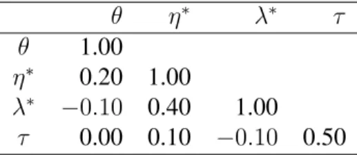
Simulated parameters for each itemiwere drawn at random and independently from these distributions: ai ∼Uniform(1,3),bi ∼Uniform(−2,2), andgi ∼Uniform(0.15,0.30), where arepresents the slope (discrimination),brepresents the threshold (difficulty), andgrepresents the lower asymptote (pseudoguessing). The simulated mean vector and variance–covariance matrix of the latent variables are informed by empirical results using the aforementioned civics and economics test data; these values appear in Tables 2.1 and 2.2.

Variable Mean θ 0.00 η∗ 1.50 λ∗ −1.25 τ 0.50

Table 2.1: The population mean of each latent variable used to generate simulated data.

θ η∗ λ∗ τ

θ 1.00 η∗ 0.20 1.00

λ∗ −0.10 0.40 1.00 τ 0.00 0.10 −0.10 0.50

(33)

3 RESULTS 3.1 Comments on the algorithms

3.1.1 MH–RM algorithm

The MH–RM algorithm with M = 1 repeatedly failed to converge, even when fitting the full model to data simulated from itself. Closer observation revealed at least part of the problem was attributable to the Metropolis–Hastings sampler becoming “stuck” in a local maximum of a multimodal likelihood surface, resulting in poor estimates of the population mean and variance of τ in particular. This scenario has longstanding precedent in the literature in educational psychology: Samejima (1973) and Yen, Burket, & Sykes (1991) noted that in a unidimensional 3PL context the likelihood overθ for some response patterns may be bimodal. An analogous

situation exists forτ in the case of the Chang et al. (2014) model as well as the full model. Increasing the value of M appeared to improve estimation of the population mean and variance ofτ somewhat, but at an increase in computation time so substantial that the EM al-gorithm would converge at least as quickly and produce better parameter estimates. Estimating the parameters of the full model with 80 items and 5,000 examinees on a 2.9–3.3 GHz Intel Xeon X5670 processor, the EM algorithm generally converged in 40–100 hours.1

3.1.2 EM algorithm

Fitting the same models (using the same data and prior densitites) with the EM algorithm achieved a 100% convergence rate in all trials with simulated and empirical data, and con-sistenly produced higher values of the log likelihood, a further indication that the MH–RM algorithm did not achieve maximum likelihood estimates as intended. Although the EM al-gorithm is also sensitive to starting values and is not immune to local solutions, Wothke et al.

1_{Convergence typically occured after 50–150 cycles, and each cycle required approximately 45 minutes of}

(34)

(2011) showed it is much more robust than stochastic algorithms. 3.2 Simulation estimates

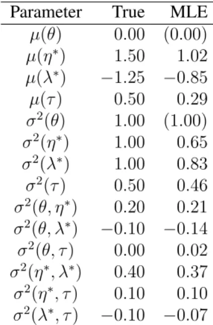
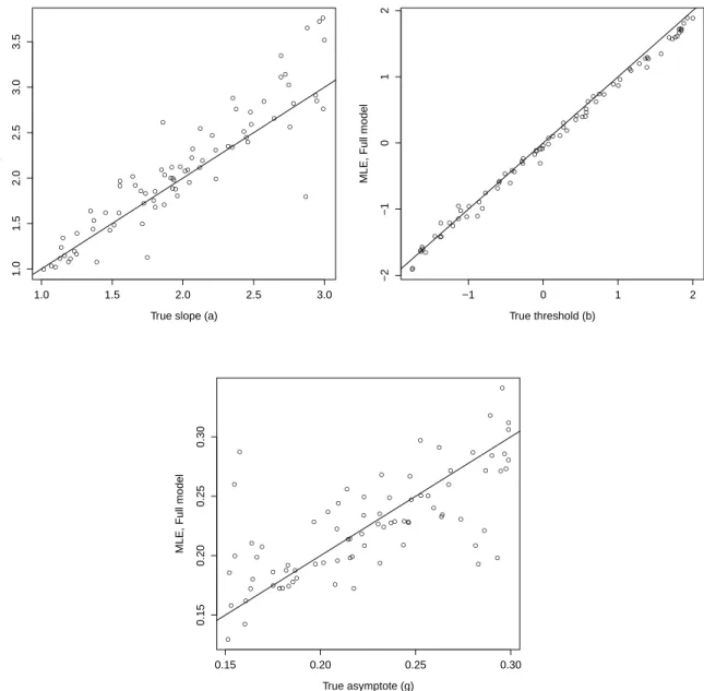
Maximum likelihood estimates of slope, threshold, and lower asymptote are plotted against their true values in Figure 3.1, in which the scatterplots with superimposed identity lines show that the parameters of data generated from and fitted with the full model are recovered in line with expectations. In addition, all estimates of population parameters (Table 3.1) match the sign of their true values.

Parameter True MLE µ(θ) 0.00 (0.00) µ(η∗) 1.50 1.02 µ(λ∗) −1.25 −0.85 µ(τ) 0.50 0.29 σ2(θ) 1.00 (1.00) σ2₍_η∗₎ ₁_.₀₀ ₀_.₆₅

σ2₍_λ∗₎ ₁_.₀₀ ₀_.₈₃

σ2(τ) 0.50 0.46 σ2₍_{θ, η}∗₎ ₀_.₂₀ ₀_.₂₁

σ2₍_{θ, λ}∗₎ ₋₀_.₁₀ ₋₀_.₁₄

σ2(θ, τ) 0.00 0.02 σ2₍_η∗_{, λ}∗₎ ₀_.₄₀ ₀_.₃₇

σ2₍_η∗_{, τ}₎ ₀_.₁₀ ₀_.₁₀

σ2(λ∗, τ) −0.10 −0.07

Table 3.1: Recovery of population parameters simulated from and fitted with the full model.

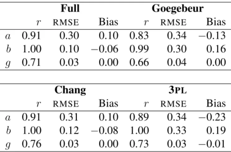
As is expected in IRT estimation, thresholds (difficulty, b) are estimated most accurately; slopes (discrimination, a) are overestimated slightly, and lower asymptotes (guessing, g) are estimated with high variability but without bias. Table 3.2 shows the correlation between item parameter estimates and their true values, along with mean squared error (MSE) and mean bias, for each of the fitted models where data were generated from the full model.

(35)

● ● ● ● ● ● ● ● ● ● ● ● ● ● ● ● ● ● ● ● ● ● ● ● ● ● ● ● ● ● ● ● ● ● ● ● ● ● ● ● ● ● ● ● ● ● ● ● ● ● ● ● ● ● ● ● ● ● ● ● ● ● ● ● ● ● ● ● ● ● ● ● ● ● ● ● ● ● ● ●

1.0 1.5 2.0 2.5 3.0

1.0 1.5 2.0 2.5 3.0 3.5

True slope (a)

MLE, Full model

● ● ● ● ● ● ● ● ● ● ● ● ● ● ● ● ● ● ● ● ● ● ● ● ● ● ● ● ● ● ● ● ● ● ● ● ● ● ● ● ● ● ● ● ● ● ● ● ● ● ● ● ● ● ● ●● ● ●● ● ● ● ● ● ● ● ● ● ● ● ● ● ● ● ● ● ● ● ●

−1 0 1 2

−2

−1

0

1

2

True threshold (b)

MLE, Full model

● ● ● ● ● ● ● ● ● ● ● ● ● ● ● ● ● ● ● ● ● ● ● ● ● ● ● ● ● ● ● ● ● ● ● ● ● ● ● ● ● ● ● ● ● ● ● ● ● ● ● ● ● ● ● ● ● ● ● ● ● ● ● ● ● ● ● ● ● ● ● ● ● ● ● ● ● ● ● ●

0.15 0.20 0.25 0.30

0.15

0.20

0.25

0.30

True asymptote (g)

MLE, Full model

Figure 3.1: Recovery of item parameters simulated from the full model, fitted with the full model.

Each plot shows the maximum likelihood estimates (on the vertical axis) of 80 slope,

(36)

Full Goegebeur

r RMSE Bias r RMSE Bias

a 0.91 0.30 0.10 0.83 0.34 −0.13 b 1.00 0.10 −0.06 0.99 0.30 0.16 g 0.71 0.03 0.00 0.66 0.04 0.00

Chang 3PL

r RMSE Bias r RMSE Bias

a 0.91 0.31 0.10 0.89 0.34 −0.23 b 1.00 0.12 −0.08 1.00 0.33 0.19 g 0.76 0.03 0.00 0.73 0.03 −0.01

Table 3.2: Recovery of item parameters simulated from the full model, fitted to various models. ris the correlation between the parameter estimates and their true values in the full model. MSE is mean squared error and Bias is mean bias relative to the same true values.

The Chang et al. (2014) model and the full model exhibit smaller errors, and as expected, the full model estimates of item thresholds exhibit the smallest bias.

The goodness-of-fit statistics in Tables 3.3–3.5 illustrate the flexibility of the Chang et al. (2014) model, which yielded better AIC and BIC values more frequently than any other model. Within each comparison of models, the best-fitting statistic is highlighted in yellow. The Goegebeur et al. (2008) model fits best when it generated the data, even by the −2 log likelihood which should always favor the model with the largest number of parameters, assum-ing all models with fewer parameters are nested. However, when data are generated from the Goegebeur et al. (2008) model, this assumption is no longer true in practice, because the only possible constraint to impose on the full model such that it reduces to the Goegebeur et al. (2008) model is to require allτ to be very large (specifically, for all individualτ values to be larger than the largestbparameter), which is precluded by the conjugate prior distribution for τ in the full model.

(37)

● ● ● ● ● ● ● ● ● ● ● ● ● ● ● ● ● ● ● ● ● ● ● ● ● ● ● ● ● ● ● ● ● ● ● ● ● ● ● ● ● ● ● ● ● ● ● ● ● ● ● ● ● ● ● ● ● ● ● ● ● ● ● ● ● ● ● ● ● ● ● ● ● ● ● ● ● ● ● ●

1.0 1.5 2.0 2.5 3.0

1.0

1.5

2.0

2.5

3.0

True slope (a)

MLE, Goegebeur et al. (2008) model

● ● ● ● ● ● ● ● ● ● ● ● ● ● ● ● ● ● ● ● ● ● ● ● ● ● ● ● ● ● ● ● ● ● ● ● ● ● ● ● ● ● ● ● ● ● ● ● ● ● ● ● ● ● ● ●● ● ● ● ● ● ● ● ● ● ● ● ● ● ● ● ● ● ● ● ● ● ● ●

−1 0 1 2

−2

−1

0

1

2

True threshold (b)

● ● ● ● ● ● ● ● ● ● ● ● ● ● ● ● ● ● ● ● ● ● ● ● ● ● ● ● ● ● ● ● ● ● ● ● ● ● ● ● ● ● ● ● ● ● ● ● ● ● ● ● ● ● ● ● ● ● ● ● ● ● ● ● ● ● ● ● ● ● ● ● ● ● ● ● ● ● ● ●

0.15 0.20 0.25 0.30

0.15

0.20

0.25

0.30

0.35

True asymptote (g)

Figure 3.2: Recovery of item parameters simulated from the full model, fitted to the Goegebeur et al. (2008) model.

(38)

● ● ● ● ● ● ● ● ● ● ● ● ● ● ● ● ● ● ● ● ● ● ● ● ● ● ● ● ● ● ● ● ● ● ● ● ● ● ● ● ● ● ● ● ● ● ● ● ● ● ● ● ● ● ● ● ● ● ● ● ● ● ● ● ● ● ● ● ● ● ● ● ● ● ● ● ● ● ● ●

1.0 1.5 2.0 2.5 3.0

1.0 1.5 2.0 2.5 3.0 3.5 4.0

True slope (a)

MLE, Chang et al. (2014) model

● ● ● ● ● ● ● ● ● ● ● ● ● ● ● ● ● ● ● ● ● ● ● ● ● ● ● ● ● ● ● ● ● ● ● ● ● ● ● ● ● ● ● ● ● ● ● ● ● ● ● ● ● ● ● ●● ● ● ● ● ● ● ● ● ● ● ● ● ● ● ● ● ● ● ● ● ● ● ●

−1 0 1 2

−2

−1

0

1

True threshold (b)

● ● ● ● ● ● ● ● ● ● ● ● ● ● ● ● ● ● ● ● ● ● ● ● ● ● ● ● ● ● ● ● ● ● ● ● ● ● ● ● ● ● ● ● ● ● ● ● ● ● ● ● ● ● ● ● ● ● ● ● ● ● ● ● ● ● ● ● ● ● ● ● ● ● ● ● ● ● ● ●

0.15 0.20 0.25 0.30

0.15

0.20

0.25

0.30

0.35

True asymptote (g)

Figure 3.3: Recovery of item parameters simulated from the full model, fitted to the Chang et al. (2008) model.

(39)

● ● ● ● ● ● ● ● ● ● ● ● ● ● ● ● ● ● ● ● ● ● ● ● ● ● ● ● ● ● ● ● ● ● ● ● ● ● ● ● ● ● ● ● ● ● ● ● ● ● ● ● ● ● ● ● ● ● ● ● ● ● ● ● ● ● ● ● ● ● ● ● ● ● ● ● ● ● ● ●

1.0 1.5 2.0 2.5 3.0

1.0

1.5

2.0

2.5

True slope (a)

MLE, 3PL model

● ● ● ● ● ● ● ● ● ● ● ● ● ● ● ● ● ● ● ● ● ● ● ● ● ● ● ● ● ● ● ● ● ● ● ● ● ● ● ● ● ● ● ● ● ● ● ● ● ● ● ● ● ● ● ●● ● ● ● ● ● ● ● ● ● ● ● ● ● ● ● ● ● ● ● ● ● ● ●

−1 0 1 2

−2

−1

0

1

2

True threshold (b)

MLE, 3PL model

● ● ● ● ● ● ● ● ● ● ● ● ● ● ● ● ● ● ● ● ● ● ● ● ● ● ● ● ● ● ● ● ● ● ● ● ● ● ● ● ● ● ● ● ● ● ● ● ● ● ● ● ● ● ● ● ● ● ● ● ● ● ● ● ● ● ● ● ● ● ● ● ● ● ● ● ● ● ● ●

0.15 0.20 0.25 0.30

0.15

0.20

0.25

0.30

True asymptote (g)

MLE, 3PL model

Figure 3.4: Recovery of item parameters simulated from the full model, fitted to the 3PL model. Each plot shows the maximum likelihood estimates (on the vertical axis) of 80 slope,

(40)

Fitted model−2LL

Full Goegebeur Chang 3PL

Simulated from Full 401341 401391 401365 401414 Simulated from Goegebeur 399061 399055 399100 401751 Simulated from Chang 399833 399837 399836 403206 Simulated from 3PL 398615 398633 398618 401419

Table 3.3: −2 log likelihood values from data simulated from and fit to various models. Fitted model AIC

Table 3.4: Akaike’s information criteria from data simulated from and fit to various models.

3.3 Empirical example

The empirical data are from the administration of five forms of a civics and economics test, each with 100 total items, of which a subset of 20 were pretest items for which there are no data available for the present study. Pretest items appeared as item numbers 21–40 on Form 1, item numbers 1–20 on Form 2, item numbers 41–60 on Form 3, item numbers 61–80 on Form 4, and item numbers 81–100 on Form 5.

Although the forms share many of the same items, the original calibration of this test treated each form separately and used all examinees (at least 20,000 per form) to obtain 3PL parame-ter estimates. These estimates are used as a standard when evaluating the parameparame-ters from the speeded models in the present study. The present study subdivides the approximately 20,000 examinees per form into four replications of 5,000 examinees chosen at random without re-placement.

Goodness-of-fit statistics for each test form, displayed in Tables 3.6–3.10, show that the full model always achieves the best −2 log likelihood. At the p = .05 level, based on the

(41)

Fitted model BIC

Table 3.5: Bayesian information criteria from data simulated from and fit to various models.

replications; and over the 3PLmodel in 18 of 20 replications.2

AIC values, which account for model parsimony through a penalty for additional param-eters, favor the full model in a majority of cases (12 of 20 replications). The AIC favored the Chang et al. (2014) model half as often (6 of 20 replications), favored the Goegebeur et al. (2008) model twice, and never favored the 3PLmodel.

BIC values, which account for sample size (number of examinees) in addition to the number of modeled parameters, exhibit the least consistency, favoring the full model twice and the Goegebeur et al. (2008) and Chang et al. (2014) models each 7 times out of 20 replications. BIC values favor the 3PLmodel in 4 of 20 replications.

Neither the AIC nor the BIC uniformly favor a single model in any of the five test forms across replications. For example, across replications of the fourth test form (Table 3.9), the AIC favors the full model in three cases and the Chang et al. (2014) model in one case, while the BIC favors the full model in one case, the Goegebeur et al. (2008) model in two cases, and the 3PLmodel in another case.

Relative to the original calibration, item parameters estimated by the full model tend to be higher for slopes and lower for thresholds, particularly for the thresholds of the most difficult items, as apparent in Figure 3.5, which plots the parameter estimates from the full model against the originally calibrated 3PL values with an identity line superimposed in each panel.

(42)

Item slopes and thresholds, but not asymptotes, from the Goegebeur et al. (2008) model very closely match their respective values from the original calibration (Figure 3.6). Table 3.11, as well as the lower panel of Figure 3.6, show that the Goegebeur et al. (2008) model has the largest root mean squared error of estimation in the asymptotes.

The Chang et al. (2014) model yields the same general pattern of results (Figure 3.7) as the full model, in which slopes are underestimated and thresholds are overestimated relative to the originally calibrated 3PL values. The upper right panel of Figure 3.7 shows that threshold overestimation among items of above-average difficulty (b > 0) in the Chang et al. (2014) model are larger than for less difficult items. While the full model also exhibited threshold overestimation, the disparity was smaller—less than triple—between above-average items and all items.

According to estimates of the means of population distributions of the latent variables in the full model (Table 3.12), the mean ofη∗ is 1.65, equivalent toη = 0.87—that is, a typical examinee begins to manifest speededness at 87% of the way through the test. The grand mean ofτ indicates that the average examinee considers an item ofb > 0.46to be difficult enough to save and return to later during the test. While η∗ and λ∗ exhibit a positive and negative correlation withθ, respectively, Table 3.13 shows that the estimate of the correlation between τ andθ is zero, on average. (Appendix A.1 displays the covariance for each of test form and replication.)

Table 3.14 demonstrates the consistency of estimates of the mean of the latent variables in the Goegebeur et al. (2008) model, across both forms and replications. The grand mean of η∗ in this model is 1.49, equivalent to η = 0.84or 84% of the way through the test, which is a 3 percentage point decrease from the same value in the full model. Table 3.15 shows that respective correlations between latent variables have the same sign, but somewhat higher magnitudes, in the Goegebeur et al. (2008) model relative to the full model.

(43)

(44)

● ● ● ● ● ● ● ● ● ● ● ● ● ● ● ● ● ● ● ● ● ● ● ● ● _● ● ● ● ● ● ● ● ● ● ● ● ● ● ● ● ● ● ● ● ● ● ● ● ● ● ● ● ● ● ● ● ● ● ● ● ● ● ● ● ● ● ● ● ● ● ● ● ● ● ● ● ● ● ● ● ● ● ● ● ● ● ● ● ● ● ● ● ● ● ● ● ● ● ● ● ● ● ● ● ● ● ● ● ● ● ● ● ● ● ● ● ● ● ● ● ● ● ● ● ● ● ● ● ● ● ● ● ● ● ● ● ● ● ● ● ● ● ● ● ● ● ● ● ● ● ● ● ● ● ● ●● ● ● ● ● ● ● ● ● ● ● ● ● ● ● ● ● ● ● ● ● ● ● ● ● ● ● ● ● ● ● ●● ● ● ● ● ● ● ● ● ● ● ● ● ● ● ● ● ● ● ● ● ● ● ● ● ● ● ● ● ● ● ● ● ● ● ● ● ● ● ● ● ● ● ● ● ● ● ● ● ● ● ● ● ● ● ● ● ● ● ● ● ● ● ● ● ● ● ● ● ● ● ● ● ● ● ● ● ● ●● ● ● ● ● ● ● ● ● ● ● ● ● ● ● ● ● ● ● ● ● ● ● ● ● ● ● ● ● ● ● ● ● ● ● ● ● ● ● ● ● ● ● ●● ● ● ● ● ● ● ●● ● ● ● ● ● ● ● ● ● ● ●● ● ● ● ● ● ● ● ● ● ● ● ● ● ● ● ● ● ● ● ● ● ● ● ● ● ● ● ● ● ● ● ● ● ● ● ● ● ● ● ● ● ● ● ● ● ● ● ● ● ● ● ● ● ● ● ● ● ● ● ● ● ● ● ● ● ● ●

0.5 1.0 1.5

0.5

1.0

1.5

2.0

3PL slope (a)

Full model slope

● ● ● ● ● ● ● ● ● ●●● ● ● ● ● ● ● ● ● ● ● ● ● ● ● ● ● ● ● ● ● ● ● ●● ● ● ● ● ● ● ● ● ● ● ● ● ● ● ● ● ● ● ● ● ● ● ● ● ● ● ● ● ● ● ● ● ● ● ● ● ● ● ● ● ● ● ● ● ● ● ● ● ● ● ● ● ● ● ● ● ● ● ● ● ● ● ● ● ● ● ● ● ● ● ● ● ● ● ● ● ● ● ● ● ● ● ● ● ● ● ● ● ● ● ● ● ● ● ● ● ● ● ● ● ● ● ● ● ● ● ● ● ● ● ● ● ● ● ● ● ● ● ● ● ● ● ● ● ● ● ● ● ● ● ● ● ● ● ● ●● ● ● ● ● ● ● ● ● ● ● ● ● ● ● ● ● ● ● ● ● ● ● ● ● ● ● ● ● ● ● ● ● ● ●● ● ● ● ● ● ● ● ● ● ● ● ● ● ● ● ● ● ● ● ● ● ● ● ● ● ● ● ● ● ● ● ● ● ● ● ● ● ● ● ● ● ●●● ● ● ● ● ● ● ● ● ● ● ● ● ● ● ● ● ● ● ● ● ● ● ● ● ● ● ● ● ● ● ● ● ● ● ● ● ● ● ● ● ● ● ● ● ● ● ● ● ● ● ● ● ● ● ● ● ● ● ● ● ● ● ● ● ● ● ● ● ● ● ● ● ● ● ● ● ● ● ● ● ● ● ● ● ● ●● ● ● ● ● ● ● ● ● ● ● ● ● ● ● ● ● ● ●● ● ● ● ● ● ● ● ● ● ● ● ● ● ● ● ● ● ● ● ● ● ● ● ● ● ● ● ● ● ● ● ● ● ● ● ● ● ● ● ● ● ●

−2 −1 0 1 2

−2

−1

0

1

3PL threshold (b)

Full model threshold

● ● ● ● ● ● ● ● ● ● ● ● ● ● ● ● ● ● ● ● ● ● ● ● ● ● ● ● ● ● ● ● ● ● ● ● ● ● ● ● ● ● ● ● ● ● ● ● ● ● ● ● ● ● ● ● ● ● ● ● ● ● ● ● ● ● ● ● ● ● ● ● ● ● ● ● ● ● ● ● ● ● ● ● ● ● ● ● ● ● ● ● ● ● ● ● ● ● ● ● ● ● ● ● ● ● ● ● ● ● ● ● ● ● ● ● ● ● ● ● ● ● ● ● ● ● ● ● ● ● ● ● ● ● ● ● ● ● ● ● ● ● ● ● ● ● ● ● ● ● ● ● ● ● ● ● ● ● ● ● ● ● ● ● ● ● ● ● ● ● ● ● ● ● ● ● ● ● ● ● ● ● ● ● ● ● ● ● ● ● ● ● ● ● ● ● ● ● ● ● ● ● ● ● ● ● ● ● ● ● ● ● ● ● ● ● ● ● ● ● ● ● ● ● ● ● ● ● ● ● ● ● ● ● ● ● ● ● ● ● ● ● ● ● ● ● ● ● ● ● ● ●● ● ● ● ● ● ● ● ● ● ● ● ● ● ● ● ● ● ● ● ● ● ● ● ● ● ● ●● ● ● ● ● ● ● ● ● ● ● ● ● ● ● ● ● ● ● ● ● ● ● ● ● ● ● ● ● ● ● ● ● ● ● ● ● ● ● ● ● ● ● ● ● ● ● ● ● ● ● ● ● ● ● ● ● ● ● ● ● ● ● ● ● ● ● ● ● ● ● ● ● ● ● ● ● ● ● ● ● ● ● ● ● ● ● ● ● ● ● ● ● ● ● ● ● ● ● ● ● ● ● ● ● ● ● ● ● ● ● ● ● ● ● ● ● ● ● ●

0.1 0.2 0.3 0.4 0.5

0.1

0.2

0.3

0.4

0.5

3PL asymptote (g)

Full model asymptote

(45)

● ● ● ● ● ● ● ● ● ● ● ● ● ● ● ● ● ● ● ● ● ● ● ● ● ● ● ● ● ● ● ● ● ● ● ● ● ● ● ● ● ● ● ● ● ● ● ● ● ● ● ● ● ● ● ● ● ● ● ● ● ● ● ● ● ● ● ● ● ● ● ● ● ● ● ● ● ● ● ● ● ● ● ● ● ● ● ● ● ● ● ● ● ● ● ● ● ● ● ● ● ● ● ● ● ● ● ● ● ● ● ● ● ● ● ● ● ● ● ● ● ● ● ● ● ● ● ● ● ● ● ● ● ● ● ● ● ● ● ● ● ● ● ● ● ● ● ● ● ● ● ● ● ● ● ● ●● ● ● ● ● ●● ● ● ● ● ● ● ● ● ● ● ● ● ● ● ● ● ● ● ● ● ● ● ● ● ●● ● ● ● ● ● ● ● ● ● ● ● ● ● ● ● _● ● ● ● ● ● ● ● ● ● ● ● ● ● ● ● ● ● ● ● ● ● ● ● ● ● ● ● ● ● ● ● ● ● ● ● ● ● ● ● ● ● ● ● ● ● ● ● ● ● ● ● ● ● ● ● ● ● ● ● ● ● ● ● ● ● ● ● ● ● ● ● ● ● ● ● ● ● ● ● ● ● ● ● ● ● ● ● ● ● ● ● ● ● ● ● ● ● ● ● ● ● ● ● ● ● ●● ● ● ● ● ● ● ●● ● ● ● ● ● ● ● ● ● ● ●● ● ● ● ● ● ● ● ● ● ● ● ● ● ● ● ● ● ● ● ● ● ● ● ● ● ● ● ● ● ● ● ●● ● ● ● ● ● ● ● ● ● ● ● ● ● ● ● ● ● ● ● ● ● ● ● ● ● ● ● ● ● ● ● ● ● ●

0.5 1.0 1.5

0.5

1.0

1.5

3PL slope (a)

Goegebeur et al.~(2008) model slope

● ● ● ● ● ● ● ● ● ●●● ● ● ● ● ● ● ● ● ● ● ● ● ● ● ● ● ● ● ● ● ● ● ●● ● ● ● ● ● ● ● ● ● ● ● ● ● ● ● ● ● ● ● ● ● ●● ● ● ● ● ● ● ● ● ● ● ● ● ● ● ● ● ● ● ● ● ● ● ● ● ● ● ● ● ● ● ● ● ● ● ● ● ● ● ● ● ● ● ● ● ● ● ● ● ● ● ● ● ● ● ● ● ● ● ● ● ● ● ● ● ● ● ● ● ● ● ● ● ● ● ● ● ● ● ● ● ● ● ● ● ● ● ● ● ● ● ● ● ● ● ● ● ● ● ● ● ● ● ● ● ● ● ● ● ● ● ● ● ● ● ● ● ● ● ● ● ● ● ● ● ● ● ● ● ● ● ● ● ● ● ● ● ● ● ● ● ● ● ● ● ● ● ● ●● ●● ● ● ● ● ● ● ● ● ● ● ● ● ● ● ● ● ● ● ● ● ● ● ● ● ● ● ● ● ● ● ● ● ● ● ● ● ● ● ● ●●● ● ● ● ● ● ● ● ● ● ● ● ● ● ● ● ● ● ● ● ● ● ● ● ● ● ● ● ● ● ● ● ● ● ● ● ● ● ● ● ● ● ● ● ● ● ● ● ● ● ● ● ● ● ● ● ● ● ● ● ● ● ● ● ● ● ● ● ●● ● ● ● ● ● ● ● ● ● ● ● ● ● ● ● ● ●● ● ● ● ● ● ● ● ● ● ● ● ● ● ● ● ● ● ●●● ● ● ● ● ● ● ● ● ● ● ● ● ● ● ● ● ● ● ● ● ● ● ● ● ● ● ● ● ● ● ● ● ● ● ● ●● ● ● ● ●

−2 −1 0 1 2

−3 −2 −1 0 1 2

3PL threshold (b)

Goegebeur et al.~(2008) model threshold

● ● ● ● ● ● ● ● ● ● ● ● ● ● ● ● ● ● ● ● ● ● ● ● ● ● ● ● ●● ● ● ● ● ● ● ● ● ● ● ● ● ● ● ● ● ● ● ● ● ● ● ● ● ● ● ● ● ● ● ● ● ● ● ● ● ● ● ● ● ● ● ● ● ● ● ● ● ●● ● ● ● ● ● ● ● ● ● ● ● ● ● ● ● ● ● ● ● ● ● ● ● ● ● ● ● ● ● ●● ● ● ● ● ● ● ● ● ● ● ● ● ● ● ● ● ● ● ● ● ● ● ● ● ● ●● ● ● ● ● ● ● ● ● ● ● ● ● ● ● ● ● ● ● ● ● ● ● ● ● ● ● ● ● ● ● ● ● ● ● ● ● ● ● ● ● ● ● ● ● ● ● ● ● ● ● ● ● ● ● ● ● ● ● ● ● ● ● ● ● ● ● ● ● ● ● ● ● ● ● ● ● ● ● ● ● ● ● ● ● ● ● ● ● ● ● ● ● ● ● ● ● ● ● ● ● ● ● ● ● ● ● ● ● ● ● ● ● ● ●● ● ● ● ● ● ● ● ● ● ● ● ● ● ●●● ● ● ● ● ● ● ● ● ● ● ●● ● ● ● ● ●● ● ● ● ● ● ● ● ● ● ● ● ● ● ● ● ● ● ● ● ● ● ● ● ● ● ● ● ● ● ● ● ● ● ● ● ● ● ● ● ● ● ● ● ● ● ● ● ● ● ● ● ● ● ● ● ● ● ● ● ● ● ● ● ● ● ● ● ● ● ● ● ● ● ● ● ● ● ● ● ● ● ● ● ● ● ● ● ● ● ● ● ● ● ● ● ● ● ● ● ● ● ● ● ● ● ● ● ● ● ● ● ● ●

0.1 0.2 0.3 0.4 0.5

0.1

0.2

0.3

0.4

0.5

3PL asymptote (g)

Goegebeur et al.~(2008) model asymptote

(46)

● ● ● ● ● ● ● ● ● ● ● ● ● ● ● ● ● ● ● ● ● ● ● ● ● ● ● ● ● ● ● ● ● ● ● ● ● ● ● ● ● ● ● ● ● ● ● ● ● ● ● ● ● ● ● ● ● ● ● ● ● ● ● ● ● ● ● ● ● ● ● ● ● ● ● ● ● ● ● ● ● ● ● ● ● ● ● ● ● ● ● ● ● ● ● ● ● ● ● ● ● ● ● ● ● ● ● ● ● ● ● ● ● ● ● ● ● ● ● ● ● ● ● ● ● ● ● ● ● ● ● ● ● ● ● ● ● ● ● ● ● ● ● ● ● ● ● ● ● ● ● ● ● ● ● ● ●● ● ● ● ● ● ● ● ● ● ● ● ● ● ● ● ● ● ● ● ● ● ● ● ● ● ● ● ● ● ● ● ● ● ● ● ● ● ● ● ● ● ● ● ● ● ● ● ● ● ● ● ● ● ● ● ● ● ● ● ● ● ● ● ● ● ● ● ● ● ● ● ● ● ● ● ● ● ● ● ● ● ● ● ● ● ● ● ● ● ● ● ● ● ● ● ● ● ● ● ● ● ● ● ● ● ● ● ● ● ● ● ● ● ● ● ● ● ● ● ● ● ● ● ● ● ● ● ● ● ● ● ● ● ● ● ● ● ● ● ● ● ● ● ● ● ● ● ● ● ● ● ● ● ● ● ● ● ● ● ● ● ●● ● ● ● ● ● ● ● ● ● ● ●● ● ● ● ● ● ● ● ● ● ● ● ● ● ● ● ● ● ● ● ● ● ● ● ● ● ● ● ● ● ● ● ● ● ● ● ● ● ● ● ● ● ● ● ● ● ● ● ● ● ● ● ● ● ● ● ● ● ● ● ● ● ● ● ● ● ● ●

0.5 1.0 1.5

0.5

1.0

1.5

2.0

3PL slope (a)

Chang et al.~(2014) model slope

● ● ● ● ● ● ● ● ● ●● ● ● ● ● ● ● ● ● ● ● ● ● ● ● ● ● ● ● ● ● ● ● ● ●● ● ● ● ● ● ● ● ● ● ● ● ● ● ● ● ● ● ● ● ● ● ● ● ● ● ● ● ● ● ● ● ● ● ● ● ● ● ● ● ● ● ● ● ● ● ● ● ● ● ● ● ● ● ● ● ● ● ● ● ● ● ● ● ● ● ● ● ● ● ● ● ● ● ● ● ● ● ● ● ● ● ● ● ● ● ● ● ● ● ● ● ● ● ● ● ● ● ● ● ● ● ● ● ● ● ● ● ● ● ● ● ● ● ● ● ● ● ● ● ● ● ● ● ● ● ● ● ● ● ● ● ● ● ● ● ● ● ● ● ● ● ● ● ● ● ● ● ● ● ● ● ● ● ● ● ● ● ● ● ● ● ● ● ● ● ● ● ● ● ● ●● ● ● ● ● ● ● ● ● ● ● ● ● ● ● ● ● ● ● ● ● ● ● ● ● ● ● ● ● ● ● ● ● ● ● ● ● ● ● ● ● ● ●●● ● ● ● ● ● ● ● ● ● ● ● ● ● ● ● ● ● ● ● ● ● ● ● ● ● ● ● ● ● ● ● ● ● ● ● ● ● ● ● ● ● ● ● ● ● ● ● ● ● ● ● ● ● ● ● ● ● ● ● ● ● ● ● ● ● ● ● ● ● ● ● ● ● ● ● ● ● ● ● ● ● ● ● ● ● ●● ● ● ● ● ● ● ● ● ● ● ● ● ● ● ● ● ● ●● ● ● ● ● ● ● ● ● ● ● ● ● ● ● ● ● ● ● ● ● ● ● ● ● ● ● ● ● ● ● ● ● ● ● ● ● ●● ● ● ● ●

−2 −1 0 1 2

−2

−1

0

1

3PL threshold (b)

Chang et al.~(2014) model threshold

● ● ● ● ● ● ● ● ● ● ● ● ● ● ● ● ● ● ● ● ● ● ● ● ● ● ● ● ● ● ● ● ● ● ● ● ● ● ● ● ● ● ● ● ● ● ● ● ● ● ● ● ● ● ● ● ● ● ● ● ● ● ● ● ● ● ● ● ● ● ● ● ● ● ● ● ●● ● ● ● ● ● ● ● ● ● ● ● ● ● ● ● ● ● ● ● ● ● ● ● ● ● ● ● ● ● ● ● ● ● ● ● ● ● ● ● ● ● ● ● ● ● ● ● ● ● ● ● ● ● ● ● ● ● ● ● ● ● ● ● ● ● ● ● ● ● ● ● ● ● ● ● ● ● ● ● ● ● ● ● ● ● ● ● ● ● ● ● ● ● ● ● ● ● ● ● ● ● ● ● ● ● ● ● ● ● ● ● ● ● ● ● ● ● ● ● ● ● ● ● ● ● ● ● ● ● ● ● ● ● ● ● ● ● ● ● ● ● ● ● ● ● ● ● ● ● ● ● ● ● ● ● ● ● ● ● ● ● ● ● ● ● ● ● ● ● ● ● ● ● ●● ● ● ● ● ● ● ● ● ● ● ● ● ● ● ● ● ● ● ● ● ● ● ● ● ● ● ●● ● ● ● ● ● ● ● ● ● ● ● ● ● ● ● ● ● ● ● ● ● ● ● ● ● ● ● ● ● ● ● ● ● ● ● ● ● ● ● ● ● ● ● ● ● ● ● ● ● ● ● ● ● ● ● ● ● ● ● ● ● ● ● ● ● ● ● ● ● ● ● ● ● ● ● ● ● ● ● ● ● ● ● ● ● ● ● ● ● ● ● ● ● ● ● ● ● ● ● ● ● ● ● ● ● ● ● ● ● ● ● ● ● ● ● ● ● ● ●

0.1 0.2 0.3 0.4 0.5

0.1

0.2

0.3

0.4

0.5

3PL asymptote (g)

Chang et al.~(2014) model asymptote

(47)

Model

Replication Full Goeg. Chang 3PL 1

−2LL 412967 412981 413144 413171 AIC 413471 413475 413630 413651 BIC 415113 415085 415213 415215

2

−2LL 410529 410563 410570 410606 AIC 411033 411057 411056 411086 BIC 412675 412666 412640 412650

3

−2LL 411558 411590 411771 411779 AIC 412062 412084 412257 412259 BIC 413704 413694 413841 413823

4

−2LL 411477 411486 411482 411501 AIC 411981 411980 411968 411981 BIC 413623 413590 413552 413545

Table 3.6: Fit indices from each replication of the first of five empirical test forms.

Model

−2LL 412702 412733 412717 412753 AIC 413206 413227 413203 413233 BIC 414849 414837 414786 414797

2

−2LL 411206 411232 411228 411262 AIC 411710 411726 411714 411742 BIC 413352 413335 413298 413307

3

−2LL 410948 410953 410954 410968 AIC 411452 411447 411440 411448 BIC 413094 413056 413024 413012

4

−2LL 412563 412569 412591 412600 AIC 413067 413063 413077 413080 BIC 414709 414672 414661 414644

(48)

Model

−2LL 417163 417183 417295 417326 AIC 417667 417677 417781 417806 BIC 419310 419287 419364 419370

2

−2LL 413401 413410 413478 413509 AIC 413905 413904 413964 413989 BIC 415547 415514 415547 415553

3

−2LL 415940 415959 416063 416104 AIC 416444 416453 416549 416584 BIC 418086 418063 418133 418148

4

−2LL 415400 415450 415557 415596 AIC 415904 415944 416043 416076 BIC 417547 417553 417626 417640

Table 3.8: Fit indices from each replication of the third of five empirical test forms.

Model

−2LL 420907 420934 421045 421062 AIC 421411 421428 421531 421542 BIC 423053 423038 423115 423107

2

−2LL 423071 423102 423214 423259 AIC 423575 423596 423700 423739 BIC 425218 425206 425283 425303

3

−2LL 420194 420222 420200 420230 AIC 420698 420716 420686 420710 BIC 422340 422326 422270 422274

4

−2LL 422591 422643 422760 422765 AIC 423095 423137 423246 423245 BIC 424738 424747 424830 424809

(49)

Model

−2LL 430811 430854 430830 430884 AIC 431315 431348 431316 431364 BIC 432957 432958 432899 432928

2

−2LL 430209 430258 430238 430295 AIC 430713 430752 430724 430775 BIC 432356 432362 432307 432339

3

−2LL 429989 430078 430004 430106 AIC 430493 430572 430490 430586 BIC 432135 432182 432074 432150

4

−2LL 430289 430358 430304 430385 AIC 430793 430852 430790 430865 BIC 432436 432461 432373 432429

Table 3.10: Fit indices from each replication of the fifth of five empirical test forms.

Slopea Thresholdb Asymptoteg

r RMSE Bias r RMSE Bias r RMSE Bias

(50)

Replication Summary

Form Variable 1 2 3 4 Mean SD

1

η∗ 2.27 1.76 1.45 1.71 1.80 0.34 λ∗ -1.68 -1.38 -1.33 -1.38 -1.44 0.16 τ 0.46 0.50 0.56 0.52 0.51 0.04

2

η∗ 1.62 1.58 1.70 1.51 1.60 0.08 λ∗ -1.38 -1.35 -1.33 -1.30 -1.34 0.03 τ 0.52 0.56 0.61 0.59 0.57 0.04

3

η∗ 1.98 1.89 2.24 2.05 2.04 0.15 λ∗ -1.42 -1.31 -1.64 -1.38 -1.44 0.14 τ 0.43 0.47 0.42 0.39 0.43 0.03

4

η∗ 1.92 1.80 1.79 1.85 1.84 0.06 λ∗ -1.57 -1.54 -1.48 -1.39 -1.49 0.08 τ 0.40 0.42 0.42 0.44 0.42 0.02

5

η∗ 0.95 0.98 0.97 0.99 0.97 0.02 λ∗ -1.02 -1.02 -1.03 -1.16 -1.06 0.07 τ 0.38 0.43 0.38 0.36 0.39 0.03

Grand Mean/SD

η∗ 1.65 0.41 λ∗ -1.35 0.19 τ 0.46 0.08

Table 3.12: Mean values of each latent variable in the full model in the population.

Mean over replications SD over replications

θ η∗ λ∗ τ θ η∗ λ∗ τ

θ 1.00 0.00

η∗ 0.31 1.18 0.32 0.60

λ∗ -0.26 0.17 1.11 0.20 0.43 0.32

τ 0.00 0.06 -0.07 0.44 0.04 0.08 0.06 0.07